Analytic algorithms for Some Models of Nonlinear Age–Structured Population Dynamics and Epidemiology

(1)

Journal of Modern Physics, 2011, 2, 236-247

doi:10.4236/jmp.2011.24033 Published Online April 2011 (http://www.SciRP.org/journal/jmp)

Analytic algorithms for Some Models of Nonlinear

Age–Structured Population Dynamics and Epidemiology

Vipul K. Baranwal, Ram K. Pandey, Manoj P. Tripathi, Om. P. Singh Department of Applied Mathematics, Institute of Technology, Banaras Hindu University,

Varanasi, India

E-mail: [email protected], [email protected]

Received January 4, 2011; revised February 7, 2011; accepted February 9, 2011

Abstract

Three analytic algorithms based on Adomian decomposition, homotopy perturbation and homotopy analysis methods are proposed to solve some models of nonlinear age-structured population dynamics and epidemi-ology. Truncating the resulting convergent infinite series, we obtain numerical solutions of high accuracy for these models. Three numerical examples are given to illustrate the simplicity and accuracy of the methods. Keywords:Age-Structured Population Models, Population Dynamics, SIS Epidemic Models, Adomian

Decomposition Method, Homotopy Perturbation and Homotopy Analysis Methods.

1. Introduction

Individuals in a structured population are distinguished by age, size, maturity and some other individual physical characteristics. The basic assumption when modelling the evaluation of such a population is that the structure of the population with respect to these individual physical characteristics at a given time, and possibly some envi-ronmental inputs as time evolves, completely determines the dynamical behaviours of the population. Mathemati-cal models describing this evolution have attracted a considerable amount of interest among scientists as a tool for modelling the interaction of different population communities in such diverse fields as demography, epi-demiology, ecology, cell kinetics, tumer growth etc.

For a long time, there has been an interest in model-ling population dynamics. The first discrete population model appears in Liber Abaci by Leonardo Pisano in 1228 [1], which gives rise to the celebrated Fibonacci sequences. The simplest continuous model is due to Malthus in 1798 [2]. His model is an unstructured one and it leads to an exponential growth of the population which is usually invalid for large time. Forty years later, in 1838, Verhulst proposed a logistic model which im-pose a maximum size for the population by considering the effects of crowding and the limitation of resources.

In order to build adequate models for population dy-namics, some detail concerning individual behaviour and its effects on vital rates of growth, production, and death

must be included. Perhaps the most natural way to con-sider such effects is to introduce the age variable into the model describing the population dynamics.

Among the first continuous population models incor-porating age effects were those of Sharpe and Lotka [3] and McKendrick [4]. Basically, the Sharpe-Lotka- McKendrick models assume that birth and mortality processes are linear functions of population density. In 1974, Gurtin and MacCamy [5] proposed a nonlinear age structured model. The allowed the mortality rate and the fertility rate to be affected by the total population, which is true for the most real cases. Their model generalizes Verhulst’s, and under reasonable assumptions on the vital rates of the population, results in a logistic model with bounded growth.

We consider the following nonlinear age–structured population model [5] and name it as model (A):

 



,



0, 0 ,

u u

x P t u x A t

t x 

 

0,

    

   (1.1)

 

, 0 0

 

, 0 ,

u x u x  x A (1.2)

 



 



 

0

0, , , d , 0,

A

u t 



 x P t u x t x t (1.3)

 

0

, d , 0,

A

P t 



u x t x t (1.4)

(2)

V. K. BARANWAL ET AL. ₂₃₇

a a

with respect to age x of a population at time t. The units of are given in units of population divided by units of time. Hence, the total number of individuals be-

 

,

u x t



u x

tween ages a and is given by

 

, d ,

a a

a

u x t x





where ,t



is taken to be smooth function of

 

x t, .

,

A

The model (A) describes the evolution of the age-density of a population, with maximum age

 

,

u x t  

whose growth is regulated by the vital rates  and  [5-7]. To be specific,  and  denote fertility and death rate respectively. If d1

 

x d2

   

x P t and then the model (A) reduces to what we call model (B):

 

b x

 ₁ b₂

   

x P t ,



 

     

1 2

d d ,

0 , 0,

u u

,

x x P t u x t

t x

x A t

 _ _{ }_ _ _

 

 

  

(1.5)

 

, 0 0

 

, 0 ,

u x u x  x A



(1.6)

 

1

 

2

     

0

0, , d , 0,

A

u t 



_b  b  P t _u  t  t (1.7)

 

0

, d , 0,

A

P t 



u x t x t (1.8)

where d1

 

x is the natural death rate (without consid-ering competition), d2

   

x P t is the increase of death rate due to competition, b x₁

 

is the natural fertility rate (without considering competition), b₂

   

x P t is the decrease of fertility rate considering competition. Equation (1.3) or (1.7), also called the renewal equation, gives the number of new born individuals introduced into the population. The value of at any time t de-pends on the age distribution of the population at that time.



0,t



u

The nonlocal boundary condition (1.7) complicates the application of standard numerical techniques such as finite difference, finite elements, spectral methods and so on [8]. So, to avoid the complexity involved in applying those numerical methods to the population model, it is important to convert the nonlocal boundary value prob-lem into more desirable forms. However, it turns out to be a hard work in many cases. Therefore, for nonlinear age-structured population models, there are only few methods for solving them. In recent years, the numerical approximation of the model (A) has been studied by sev-eral authors like Abia and Lopez–Marcos, they applied difference schemes based on Runge–Kutta method and other numerical integration techniques to solve it [9-11]. In [12], Kim and Park developed an upwind scheme for the model (A). Iannelli et al. [13] solved it by using split-ting methods. Reproducing kernel method was success-fully applied by Cui and Chen [14] and Krzyzanowski et

al. gave a discontinuous Galerkin method for non linear age structured population model [15]. Norhayati and Wake [16] used Laplace transform technique to solve and analysed the existence of steady age distribution and its stability.

Recently methods like Adomian decomposition method (ADM), homotopy perturbation method (HPM), homo-topy analysis method (HAM) have been used success-fully to solve a variety of non linear problems [17-20]. Dehghan and Salehi [21] used VIM and ADM to solve the delay logistic equation which has been extensively used as models in biology with particular emphasis on population dynamics. In 2009, Li [8] applied VIM to solve the model (B) with great success, but ADM, HPM and HAM have yet not been used for the purpose.

The aim of the present paper is to apply these tech-niques for the numerical evaluation of the non linear age-structured population model (B). The basic ideas of these methods apply to other problems related to (B). In fact the same approaches are used for approximation of the age-structured SIS model.

The paper is organized as follows. In sections 2-4, we introduce the algorithms based on ADM, HPM and HAM respectively. In sec. 5, we apply these algorithms on some numerical experiments and finally conclusions are given in sec. 6.

2. Adomian Decomposition Method (ADM)

In this section we give a brief outline of ADM for solv-ing nonlinear age–structured population model (NASPM). Equation (1.5) may be written in the operator form as

 







 



   

 



 



1 2

, , d

d , 0,

t x

L u x t L u x t x u x t

x N u x t

 

 

,

(2.1)

where the notations Lt t  

 and Lx x  

 symbolize

the linear differential operators and the notation

symbolizes the

nonlin-ear operator.

 





   

0

, , ,

A

N u x t u x t



u x t dx

The inverse operator Lt1



, is defined by 1

   

0

d

t

L   



. Thus, applying the inverse operator to Equation (2.1), we get

1

 t

L

 



 



   

 



 



1

1 2

, , 0 ,

d , d ,

t x

u x t u x L L u x t

x u x t x N u x t

 _

  _



  _.

(2.2)

(3)

V. K. BARANWAL ET AL. 238

, [17,18]. For a given nonlinear operator N u x t



 

,



,

these polynomials are calculated using the basic formula:

 

0

, _n

n

u x t u x t

 





. (2.3) The nonlinear operator N u x t



 

,



, n ,

is decomposed as

_

_

0 1 2

0 ₀

1 d

, , , , , 0.

! d

n

k

n n n k

k

A u u u u N u n

n   _



 _

  

 _ _ __ 

 









(2.5)

 







0 1 2

0

, n , , ,

n

N u x t A u u u u

 





 (2.4)

The above formula is used to set a computer code to compute the various Adomian polynomials An. The first few polynomials are given as follows:

where An is an approximate Adomian’s polynomial

which can be calculated for all forms of nonlinearity ac-cording to specific algorithms constructed by Adomian

 

12

 

13

0 0 , 1 0 1, 2 0 2 0 , 3 0 3 0 1 2 0

2! 3!

u u

A N u A N u u A N u u N u A N u u N u u u N u ,.

0

n n





Substituting (2.3) and (2.4) in (2.2), we get

 

1

 



1 2

0 0 0

, 0 d d .

n t x n n

n n n

u u x L L u x u x A

  



  

 

  _   _

 



(2.6)

Identifying the zeroth component by the ini-tial condition we obtain the subsequent

com-ponents by the following recursive formula

 

0 ,

u x t

 

, 0 , u x

 

1



 



   

 



0 , , 0 , n1 , t x n , d1 n , d2

u x t u x u x t  L L u x t  x u x t  x An . (2.7)

We construct a homotopy v r p

 

, :

 

0,1 R sat- isfying

3. Homotopy Perturbation Method (HPM)



 

  

 

 

0

, 1

0,1 , .

H v p p L v L u p A v f r

p r

 

In this method, using the homotopy technique of topol-ogy, a homotopy is constructed with an embedding pa-rameter p

 

0,1 which is considered as a “small pa-rameter”. This method became very popular amongst the scientists and engineers, even though it involves con-tinuous deformation of a simple problem into a more difficult problem under consideration. Most of the per-turbation methods depend on the existence of a small perturbation parameter but many nonlinear problems have no small perturbation parameter at all. Many new methods have been proposed in the late nineties to solve such nonlinear equation devoid of such small parameters. Late 1990s saw a surge in applications of homotopy the-ory in the scientific and engineering computations [19]. When the homotopy theory is coupled with perturbation theory it provides a powerful mathematical tool. To il-lustrate the basic concept of HPM, consider the follow-ing nonlinear functional equation

0,

  _  _ _  _

  



(3.2) Hence,

 

,

   

0

 

0

 

0 H v p L v L u pL u p N v_  f r _ ,

(3.3) where 0 is an initial approximation for the solution of

(3.1). As

u

 

, 0

 

0 and

 

,1

 

,

H v L v L u H v A v  f r (3.4)

it shows that H v p



,



continuously traces an implicitly defined curve from a starting point to a solu-tion



0, 0

H u



 

,1

H v . The embedding parameter p increases monotonously from zero to one as the trivial linear part

 

0

L u  deforms continuously to the original problem

 

.

A u  f r The embedding parameter p

 

0,1 can be considered as an expanding parameter [19] to obtain

 

, ,

A u  f r r 

2

0 1 2 .

vv pv p v  (3.5) with the boundary conditions B u, u 0, r

n 

 _{ } _{  }

 _ 

  , _{The solution is obtained by taking the limit as}_p_tends

to 1 in equation.(3.5). Hence (3.1)

where A is a general functional operator, B is a boundary operator, f r

 

is a known analytic function, and  is the boundary of the domain . The operator A is decomposed as



,

A L N where L is the linear and N is the nonlinear operator. Hence Equation (3.1) can be writ-ten as

0 1 2 1

lim .

p

u v v v v



     (3.6) The series (3.6) converges for most cases and the rate of convergence depends on A u

 

 f r

 

.

For nonlinear age-structured population model, we choose the initial approximation u0

 

x t, u0

 

x , and construct the following homotopy:

 

0, .

(4)

V. K. BARANWAL ET AL. ₂₃₉





 

0

 

   

 

1 2

0

, , , ,

1 d d

A

v x t u x t v x t v x t

p p x x v x t x

t t t x

 

   

   

  _  _  _ _  _    _

 

  



, d v x t, 0, (3.7)

which is equivalent to

 

0

 

0

 

_{ }

_{   }

_{ }

1 2

0

, , , ,

d d , d ,

A

v x t u x t u x t v x t

p p x x v x t x v x t

t t t x

 

     

   _    _

   _  _



_ _0, (3.8)

where p

 

0,1 is an embedding parameter. Using the parameter p, we expand the solution in the following form

 

2

 

3

 

0 1 2 3

, , , , ,

v x t v x t pv x t p v x t p v x t . (3.9) Substituting Equation (3.9) into Equation (3.8), and equating the terms with the identical powers of p, we obtain:

 

_{ }

 

_{   }

_{ }

 

_{   }

_{ }

_{     }

 

0 0

0

1 0 0

1

1 0 2 0 0 1

0

2 1

2

1 1 2 1 0 2 0 1

0 0

2

3 2

3

, ,

: 0, , 0 , 0 ,

, , ,

: d , d , , d 0,

, ,

: d , d , , d d ,

( , 0) 0,

, ,

:

A

A A

v x t u x t

p v x u x

t t

u x t u x t v x t

p x v x t x v x t v x t x v x

t t x

v x t v x t

p x v x t x v x t v x t x x v x t v x t x

t x

v x

v x t v x t

p t

 

  

 

  

     

  

 

   

 



 



 



, 0 0,

, d 0,

   

 

     

   

 

1 2 2 2 0 2 1 1

0 0

2 0 2 3

0

d , d , , d d , , d

d , , d 0, ( , 0) 0, .

A A

A

x v x t x v x t v x t x x v x t v x t x

x

x v x t v x t x v x

  

  





(3.10)

We use the iterative scheme (3.10) to compute the various ’s. Hence the solution of Equation (1.5) is given by,

i

v

 

1

0

, lim , _m ,

p

m

u x t v x t v x t



 _

 



. (3.11)

4. Homotopy Analysis Method (HAM)

Homotopy analysis method (HAM) was first proposed by Liao [20] based on homotopy, a fundamental concept in topology and differential geometry. The HAM is based on construction of homotopy which continuously deforms an initial guess approximation to the exact solu-tion of the given problem. An auxiliary linear operator is chosen to construct the homotopy and an auxiliary linear parameter is used to control the region of convergence of the solution series, which is not possible in the other methods like perturbation techniques, homotopy pertur-bation methods, decomposition methods. The HAM pro-vides the greater flexibility in choosing initial approxi-mations and auxiliary linear operators and hence a com-plicated nonlinear problem can be transformed into infi-nite number simpler, linear sub problems as shown by Liao and Tan [22].

Here we give a brief description of HAM [20] to

han-dle the general non linear problem,

 

, 0, N u x t_ _ t0,



(4.1)

where N is a nonlinear operator and is unknown function of the independent variables



, u x t

, .

x t Liao [20] constructed the zero order deformation equation









 





0

1 , ;

, , ;

q L x t q u x t q H x t N x t q



  ,

,

 

 

  _ _ (4.2)

where q

 

0,1

0

is the homotopy or embedding pa-rameter,  is an auxiliary parameter, H x t

 

, 0

an auxiliary function, L is an auxiliary linear operator,

 

t

0 , an initial guess of and

u x u x t



,







x t q, ;



is

an unknown function.

Putting q0, and q1, in Equation (4.2), we see that



x t, ; 0



u0

 

x t, ,

  (4.3)



x t, ;1



u x t

 

, ,

  (4.4)

Therefore, according to Equations (4.3) & (4.4),



x t q, ;



 deforms continuously from the initial guess

 

0 ,

u x t to the exact solution as the embedding parameter q increases from 0 to 1. Liao [20] expanded

 

, u x t



x t q, ;



(5)

240 V. K. BARANWAL ET AL.





0

 

1

, ; , , m,

m m

x t q u x t u x t q

 



 



(4.5) where

 





0 , ; 1 , ! m m m q x t q u x t

m q





 

 . (4.6)

The convergence of the series (4.5) is controlled by . Assume that the auxiliary parameter the auxiliary function H, the initial approximation and the auxiliary linear operator L are so properly chosen that the series (4.5) converges at



,



0

u

 

x,t , 1.

q Then, at q1 and using (4.4) the series (4.5) gives the exact solution

as



, u x t



, .



 

0

 

1

, , _m

m

u x t u x t u x t



 



 (4.7) The above expression provides us with a relationship between the initial guess and the exact solution

by means of the terms

 

0 ,

u x t



,

u x t u_m

 

x t, m1, 2, 3,



,

, , which are still to be determined. The process of their evaluations is given as follows :

Differentiating the zero order deformation Equation (4.2) m times with respect to embedding parameter q, then setting and dividing by we get the following -order deformation equation,

0 q h !, m mt

 

, 1

 

,

 



1

 



m m m m m

L u x t  u  x t H t R u  x t (4.8)

where



1

_{  }

1



1



0

, ; 1

1 !

m

m m m

q

N x t q

R m q       _ _   

u , (4.9)

     





0 , , 1 , , 2 , ,



m u x t u x t u x t um x t

u



, (4.10)

0, 1 1, m m otherwise  _{ } 

 . (4.11)

For any given operators L and N we get the mth order deformation Equation (4.8) and solving it we get differ-ent The solution of problem (4.1) is obtained by putting these ’s in (4.7) and choosing a suit-able value of for the convergence of the series. The symbolic computation software like Maple and Mathe-matica can solve (4.8) easily.

 

, .

m

u x t



,

m

u x t



5. Numerical Applications

In this paper, we apply ADM, HPM and HAM to solve the nonlinear age-structured population models. In the following examples will denote an approxi-mate solution of the problem under consideration, ob-tained by truncating the solution series (4.7) at level

 

,

n

u x t

.

[image:5.595.58.285.83.159.2]

mn Also E_n

 

  u_exact

 

x t, u_n

 

x,t denotes the error between exact and approximate solution at . In

Table 1, 1 denote the error between exact solution

and approximate solution obtained by reproducing kernel method [14].



E

Example 5.1 Consider the following nonlinear age- structured population model [8, 14].

 

,

 

,

_{   }

, , 0, 0

u x t

P t u x t t x

t x

 

, A u x t

(5.1)

     

 

 

e

, 0 , 0 ,

2

x

u x x A



   (5.2)

 

0,

 

, 0,

u t P t t (5.3)

 

0

, d , 0,

A

P t 



u x t x t (5.4)

where, A , with

 

, e , 0, 0,

d , 1 e

x

t

u x t t x

 

  

 as

the exact solution of (5.1).

Case (a) Solution by ADM

Rewriting Equation (5.1) in the operator form

 

     

0

, , , ,

A

tu x t  L u x tx u x t



u x t x

L (5.5)

taking the initial approximation 0

 

e ,

x

, 2

u x t 

 and us-

ing the recursive formula (2.7), we find that all the even iterates u2n 0,n0,1, 2, 3, and

 

3

1 3 e e , , , 4 4 x , 8 x

u x t t u x t t

 

  

 

5

 

7

5 7

e e

, , , , .

480 80640

x x

u x t t u x t t

 

   

Hence, the solution is given by

 

0

3 5 7

, lim ,

1 e

2 4 48 480 80640

e , 1 e N n N n x x t

u x t u x t

t t t t

         _      _    





which is the exact solution.

Case (b) Solution by HPM

Taking the same initial approximation 0

 

e 2

, ,

x u x t





and using the equations (3.10), we find that all the even terates

(6)

V. K. BARANWAL ET AL. ₂₄₁

Table 1. Comparison between HAM and reproducing kernel method solutions.

Nodes

t x

Exact Solution  ,

u x t

Approximate Solution  

7 , ,

u x t  1

Error

     

7 1 , 7 ,

E  u x t u xt

Error [14]

1

E

0.00 0.00 0.5 0.5 0 0

0.20 0.00 0.549834 0.549834 1.08906E11 2.6162E02

0.40 0.00 0.598688 0.598688 5.50928E09 4.4321E02

0.60 0.00 0.645656 0.645656 2.07654E07 4.4703E02

0.80 0.00 0.689974 0.689972 2.69192E06 3.6536E02

1.00 0.00 0.731059 0.731039 1.93921E05 1.1234E02

0.00 1.00 0.18394 0.18394 0 0

0.20 1.00 0.202273 0.202273 4.00643E12 6.467E03

0.40 1.00 0.220245 0.220245 2.02675E09 1.2146E02

0.60 1.00 0.237524 0.237524 7.63918E08 1.4046E02

0.80 1.00 0.253827 0.253826 9.90302E07 7.887E03

1.00 1.00 0.268941 0.268934 7.13396E06 5.552E03

0.00 2.00 0.0676676 0.0676676 0 0

0.20 2.00 0.0744119 0.0744119 1.47389E12 5.5869E03

0.40 2.00 0.0810236 0.0810236 7.456E10 9.6181E03

0.60 2.00 0.0873801 0.0873801 2.8103E08 1.03579E02

0.80 2.00 0.0933779 0.0933775 3.64312E07 5.4159E03

1.00 2.00 0.098938 0.0989354 2.62444E06 6.5159E03

0.00 3.00 0.0248935 0.0248935 0 0

0.20 3.00 0.0273746 0.0273746 5.42216E13 4.4722E03

0.40 3.00 0.0298069 0.0298069 2.74291E10 7.3509E03

0.60 3.00 0.0321453 0.0321453 1.03385E08 8.2104E03

0.80 3.00 0.0343518 0.0343517 1.34023E07 6.4072E03

1.00 3.00 0.0363973 0.0363963 9.65477E07 2.9965E03

0.00 4.00 0.00915782 0.00915782 0 0

0.20 4.00 0.0100706 0.0100706 1.99471E13 1.8242E03

0.40 4.00 0.0109653 0.0109653 1.00906E10 3.2864E03

0.60 4.00 0.0118256 0.0118256 3.80332E09 3.7749E03

0.80 4.00 0.0126373 0.0126373 4.93043E08 3.1609E03

1.00 4.00 0.0133898 0.0133894 3.55179E07 1.8526E03

0.00 5.00 0.00336897 0.00336897 0 0

0.20 5.00 0.00370475 0.00370475 7.33805E14 3.3172E04

0.40 5.00 0.00403393 0.00403393 3.71212E11 2.5414E04

0.60 5.00 0.0043504 0.0043504 1.39916E09 1.3464E04

0.80 5.00 0.00464901 0.00464899 1.8138E08 3.5880E04

1.00 5.00 0.00492583 0.0049257 1.30663E07 8.72E04

0.00 6.00 0.00123938 0.00123938 0 0

0.20 6.00 0.0013629 0.0013629 2.69953E14 8.9154E04

0.40 6.00 0.001484 0.001484 1.36561E11 2.3233E03

0.60 6.00 0.00160042 0.00160042 5.14724E10 3.85194E03

0.80 6.00 0.00171028 0.00171027 6.67261E09 5.38069E03

1.00 6.00 0.00181211 0.00181206 4.80683E08 6.49366E03

0.00 8.00 0.000167731 0.000167731 0 0

0.20 8.00 0.000184449 0.000184449 3.65338E15 4.58849E03

0.40 8.00 0.000200837 0.000200837 1.84816E12 6.31876E03

0.60 8.00 0.000216594 0.000216593 6.96603E11 9.81151E03

0.80 8.00 0.000231461 0.00023146 9.03039E10 1.30453E02

1.00 8.00 0.000245243 0.000245236 6.50533E09 1.6041E02

0.00 10.00 0.0000227 0.0000227 0 0

0.20 10.00 0.0000249624 0.0000249624 4.94433E16 2.14306E04

0.40 10.00 0.0000271804 0.0000271804 2.50121E13 1.14205E03

0.60 10.00 0.0000293128 0.0000293127 9.42749E12 2.52654E03

0.80 10.00 0.0000313248 0.0000313247 1.22213E10 3.89648E03

1.00 10.00 0.00003319 0.0000331891 8.80401E10 5.20734E03

(7)

V. K. BARANWAL ET AL.

242

 

3

1 3

5 7

e e

, , , ,

4 48

e e

, , ,

480 80640

x x

v x t t v x t t

v x t t v x t t

 

  

   ,.

Thus we see that the various terms obtained by using HPM are same as those obtained by using ADM. In gen-eral, the ADM solution is a part of HPM solution.

Substituting these values in Equation (3.11), the solu-tion is given by

 

1

0

3 5 7

, lim , lim ,

1 e

2 4 48 480 80640

e , 1 e

N

n

p N

n

x

t

u x t v x t v x t

t t t t

 _{ }



 

 

 

 _      _

 

 





Case (c) Solution by HAM

Choosing the linear operator as L t

 

 and using the

Equations (4.8-4.10), we obtain the following or-der deformation equation as

mth

 

1 1

0

0 1 1

1 0

, ,

,

1, 2, 3,

, ,

, , d d

.

t

m m

A m

i

m m m

m i i

u x u x

x

u

u x t

x u

x t

m

u x

x  





  

 



  



 





 _ _





 _





 

_





 

(5.6)

Taking the initial guess as 0

 

,

 

, 0

2 e

,

x

u x t u x



 

and solving the Equation (5.6), we get the follow-ing

mth

 





 





1

2

2 3 3 3

e

, ,

4 e

, 1 ,

4

e e

, 1 ,

4 48

x

x x

u x t t

u x t t

u x t t t



 

 

  

   



 

   .

, ,



Truncating the series (4.7) at level m = 7, we obtain an approximate solution of (5.1) as

 

7

 

7 0

1

, , m

m

u x t u x t u x t



 





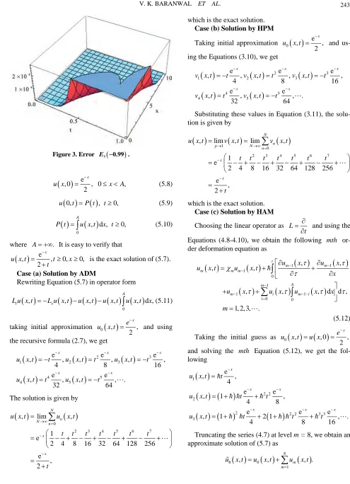
the accuracy of approximation is controlled by the auxil-iary parameter  as illustrated by Figures 3 and 4.

The approximate solution u_m



x t, converges to the

exact solution e , 1 e

x

t 



 as m  for  1.

The ADM and HPM solutions are obtained by taking 1

 

[image:7.595.90.258.81.134.2]

 in HAM solution.

[image:7.595.312.539.251.491.2]

Table 1 shows that the approximate solution u7

 

x t, obtained by HAM for  1 is more accurate com-pared to that obtain by reproducing kernel method [14].

Figure 1 shows the approximate solution for  1 ( 0.99)

, whereas Figures 2, 3 show the errors for dif-ferent values of It is observed that

 

7

E 

7

E

.

  is

smaller than E7( 1).

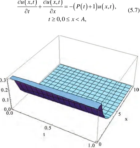
Example 5.2 Consider the following nonlinear age- structured population model [8,13].

 

,

 

,

_

_{ }

_

_{ }

1 ,

0, 0 ,

u x t u x t

P t u x t

t x

t x A

 

   

 

  

,

(5.7)

[image:7.595.313.538.526.701.2]

Figure 1. Approximate solution u7

 

x t, ,  1.

(8)

[image:8.595.43.538.57.741.2]

V. K. BARANWAL ET AL. ₂₄₃

Figure 3. Error E7



0.99



.

 

e

, 0 , 0 ,

2

x

u x x A



   (5.8)

 

0,

 

, 0,

u t P t t (5.9)

 

0

, d , 0,

A

P t 



u x t x t (5.10) where A . It is easy to verify that

 

e

, , 0, 0,

2

x

u x t t x

t 

  

 is the exact solution of (5.7). Case (a) Solution by ADM

Rewriting Equation (5.7) in operator form

 

       

0

, , , , ,

A

t x

L u x t  L u x t u x t u x t



u x t d , (5.11) x

taking initial approximation 0

 

,

2 ,

x e u x t



 and using

the recursive formula (2.7), we get

 

2

1 2 3

4 5 4 5 e e , , , , , 4 8 e e , , , , . 32 64 3e , 16 x x x x

u x t t u x t t u x t t

u x t t u x t t

             x 

The solution is given by

 

0

2 3 4 5 6 7

, lim ,

1 e

2 4 8 16 32 64 128 256

e , 2 N n N n x x

u x t u x t

t t t t t t t

t         _         _   



 

hich is the exact solution. w

Case (b) Solution by HPM

Taking initial approximation 0

 

e

, ,

2

x u x t



 and us-

ing the Equations (3.10), we get

 

2 3

1 2 3

4 5

e e e

, , , , , ,

4 8 16

e e

, , , , .

32 64

x x x

x x

v x t t v x t t v x t t

v x t t v x t t

 

    

   

Substituting these values in Equation (3.11), the solu-tio



n is given by

 

1

0

2 3 4 5 6 7

, lim , lim ,

1 e

2 4 8 16 32 64 128 256

e , 2 N n p N n x x

u x t v x t v x t

t t t t t t t

t  _{ }                     





as

Case (c) Solution by HAM

Choosing the linear operator L t  

 and using the

Equations (4.8-4.10), we obtain the following mth or-der deformation equation as

 

1 1 0 1 1 1 0 0 1 , ,

, , , d

.

, ,

,

1, 2, 3,

d m m A m m m

i m i

i m m

u x u x

x

u x

u x t u x t

u u

m

x x x

 t                     _ _         







  (5.12)

Taking the initial guess as 0

 

,

 

, 0

2

x e

,

u x t u x  and solving the mth Equation (5.12), we get the fol -lowing

 

  



  







1 2 2 2

2 2 2 3 3

3

e

, ,

4

e e

, 1 ,

4 8

e e

, 1 2 1 ,

4 8

x

x x

u x t t

u x t t t

u x t t t t

                 

     e .

16

x



Truncating the series (4.7) at level m = 8, we obtain an ap

, . proximate solution of (5.7) as

 

u x t u x t 

 

8

8 0

1

, , m

m

u x t 



(9)

The approximate solution converges to the

exact solution

 

,

m u x t

[image:9.595.312.537.76.265.2]

e , 2t

Figure 4 shows the approx lution for 1

x 

as m  for imate so

1.

  

   ,

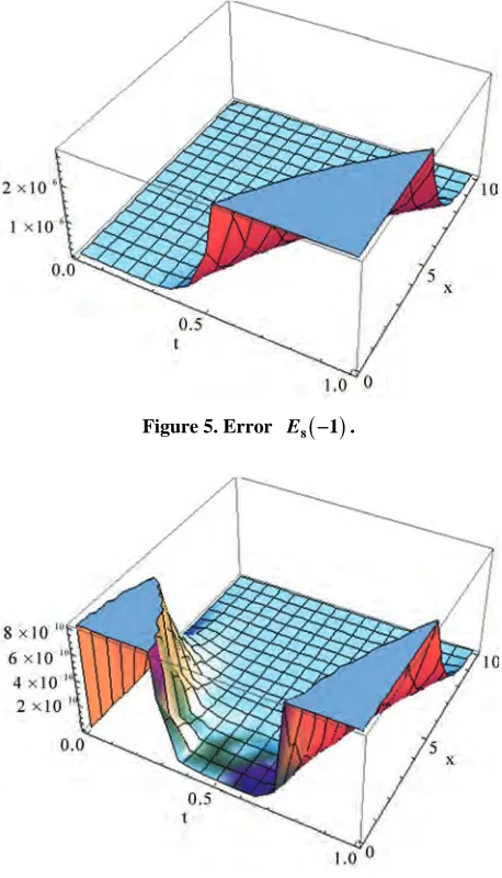
or dif-905) is whereas Figures 5, 6 show the errors f fere

lu nlethal dise

 

8

E 

SIS m nt values of . It is observed that E8( 0.7

smaller than E8( 1).

In the next example, we consider a odel de-scribing the evo tion of a human no ase which does not impo t immunity [23-25]. Some infec-r tions, for example the group of those responsible for the common cold, do not confer any long lasting immunity. Such infections do not have a recovered state and indi-viduals become susceptible again after infection. Maybe, the most specific parameter of biological system is the age, and, especially for some infectious diseases, it has a deep influence on the dynamics of its spreading in a population. Many of the parameters may depend on age, especially the contact rate, which summarizes the ‘infec-tious effectiveness’ of contacts between susceptible and infectious subjects. This effectiveness has, thus, to take into account both the age of the infectious and the age of the susceptible. Epidemic models modelling the age structure of a population are very complex. Example (5.3) illustrates the utility of our algorithm on such types of complex models.

Example 5.3 We consider the following age-structured SIS model [13]:

 

,

 

, 1

_{ }

_

_{   }

_

_{ }

, , , ,

u x t u x t

u x t i x t u x t P t

t x



   

  1

0, 0 ,

x

t x A





  

(5.13)

(5.14)



where

 

, 0 2 1





, 0 ,

u x  x  x A

 

   

0

0, , , d ,

A

u t 



 x i u x t x t0, (5.15)

 

0

, d , 0.

A

P t 



u x t x t (5.16)





2

1, 4 1

A  x or  πsinπx.

take a steady state

distri-Fo we

ch that

r the total population,

bution su i x t

 

, 4 1



x



. Then the exact solution of (5.13) is

 

, 4 1



₂_t



.

1

x u x t 

Following the in the previous

ex-e 

procedures adopted

the three methods and obtain the vari-ou



amples, we apply

s iterates of the solution as follows:

As ADM and HPM iterates are identical for p1,

we list them once.

1) ADM and HPM iterates

Figure 4. Approximate solution u8

 

x t, ,  1.

 

8 1

[image:9.595.310.539.303.703.2]

E  . Figure 5. Error

(10)

V. K. BARANWAL ET AL. ₂₄₅

 



  





 



  





0 1

3 5

7 9

11

11 2

, 2 1 , , 2 1 ,

2 4

, 1 , , 1

3 15

34 124

( , ) (1 ), ( , ) (1 ),

315 2835

3268

( , ) (1 ), ( , ) 0, 1, 2, .

155925 n

u x t x u x t t x

u x t t x u x t t x

u x t t x u x t t x

u x t t x u x t n

   

    

     

,

The solution is given by

 









0

3 5 7 9 11

2

, lim ,

2 17 62 1634

2 1 1

3 15 315 2835 155925

4 1 , 1 e

N

n N _n

t

u x t u x t

t t t t t

x t

x  

 



  _       

  







2) HAM iterates

  

 





 





 



 



 



 







 



 







0 1 2

2 _{3 3}

3

3 3 3

4

, 2 1 ,

, 2 1 1 ,

2

, 2 1 1 1 ,

3

, 2 1 1 2 1 1 , .

u x t x

u x t t x

u x t t x

u x t t x t x

 

  

   

     

      

  

    

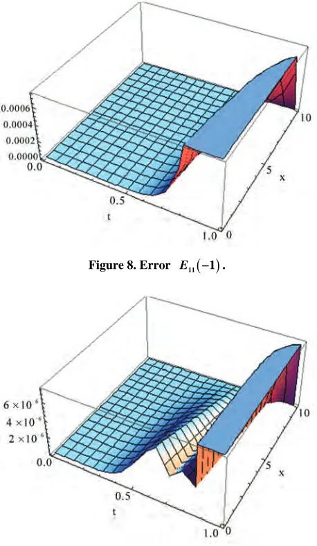
Truncating the series (4.7) at the level m = 11, we ob-tain an approximate solution of (5.13) as

, .

The approximate solution converges to the

ex

 

11

 

11 0

1

, , _m

m

u x t u x t u x t



 





 

,

m

u x t

act solution 4 1



₂_t



, 1 e

x



 

[image:10.595.311.537.71.270.2] [image:10.595.57.285.79.406.2]

as m  fo

Figure 7 shows the approximate solution for r 1.

1  

 , for

dif-.95312)

whereas Figures 8, 9 show the errors ferent values of It is observed th is smaller than

6. Conclusion

In this paper, we have given three simple, easy to im-pl

rithms involve infinite convergent series and in many cases, the closed form solutions are obtained. Where the closed form

ana-ly ailab

th xperime

ies at rel lower l of tru cation give fairly accurate solutions. Moreover, the accuracy of

 

11

E 

at E11( 0

.



11

E ( 1).

ement analytic algorithms based on ADM, HPM and HAM for nonlinear models of age-structured population dynamics and epidemiology. These algo

tical solutions are not readily av le, it is established rough the three numerical e nts that truncating the solution ser atively leve n

[image:10.595.310.539.308.702.2]

Figure 7. Approximate solution u₁₁

 

x t, ,  1.

Figure 8. Error E11

 

1 .





11 0.95312

E  .

(11)

e solution may be increased by the suitable choice of the auxiliary parameter in HAM. Table 1 clearly establishes the accuracy of our method compared to that of the reproducing kernel method proposed by Cui and Chen [14].

7. Acknowledgements

The first and third authors acknowledge the financial support from UGC and CSIR New-Delhi, India, respec tively under JRF schemes.

8. References

[1] L. Sigler, F. L. Abaci, “A Translation into Modern lish of Leonardo Pisano’s Book of Calculation, Springer-Verlag, New-York, 2002.

[2] T. R. M the Principle of Population,

,” Philosophical Magzine, Vol. 21, No. 124, 1911,

lications of Mathematics to

th



- Eng-”

althus, “An Essay on

St. Paul’s, London,” 1798, In: T. R. Malthus, “An Essay on the Principle of Population and A Summary View of the Principle of Population,” Penguin, Harmondsworth, England, 1970.

[3] F. R. Sharpe and A. J. Lotka, “A Problem in Age Distri-butions

pp. 435-438.

4] A. G. McKendrick, “App [

Medical Problems,” Proceedings of Edinburgh Mathe-matical Society, Vol. 44, 1926, pp. 98-130.

doi:10.1017/S0013091500034428

5] M. E. Gurtin and R. C. M

[ acCamy, “Nonlinear Ag

ynamics,” Archive for Rational Analysis, Vol. 54, No. 3, 1974, pp. 281-300.

cerche, Pisa, 1995.

Models,” Computers and

e-De-pendent Population D

Mechanics and

[6] M. Iannelli, “Mathematical Theory of Age-Structured Population Dynamics,” Applied Mathematics Monographs, Vol. 7, Consiglio Nazionale delle Ri

[7] G. F. Webb, “Theory of Nonlinear Age-Dependent Popu-lation Dynamics,” Marcel Dekker, New York, January 1985.

[8] X. Y. Li, “Variational Iteration Method for Nonlinear Age-Structured Population

Mathematics with Applications, Vol. 58, No. 11-12, 2009, pp. 2177-2181. doi:10.1016/j.camwa.2009.03.060

[9] L. M. Abia and J. C. Lopez-Marcos, “Runge-Kutta Meth-ods for Age-Structured Population Models,” Applied Numerical Mathematics, Vol. 17, No. 1, 1995, pp. 1-17.

doi:10.1016/0168-9274(95)00010-R

[10] L. M. Abia and J. C. Lopez-Marcos, “On the Numerical

.1016/S0025-5564(98)10080-9

Integration of Non-Local Terms for Age-Structured Population Model,” Mathematical Biosciences, Vol. 157, No.1, 1999, pp. 147-167.

doi:10

p [11] L. M. Abia, O. Angulo and J. C. Lopez-Marcos, “Age-

Structured Population Models and Their Numerical Solu-tion,” Ecological Modelling, Vol. 188, No. 1, 2005, p . 112-136. doi:10.1016/j.ecolmodel.2005.05.007

[12] M. Y. Kim and E. J. Park, “An Upwind Scheme for a Nonlinear Model in Age-Structured Population Dynam-ics,” Computers and Mathematics with Applications, Vol. 30, No. 8, 1995, pp. 5-17.

doi:10.1016/0898-1221(95)00132-I

[13] M. Iannelli, M. Y. Kim and E. J. Park, “Splitting Method for the Numerical Approximation of Some Models of Age-Structured Population Dynamics and Epidemiol-ogy,” Applied Mathematics and Computation, Vol. 87, No. 1, 1997, pp. 69-93.

doi:10.1016/S0096-3003(96)00222-6

[14] M. G. Cui and C. Chen, “The Exact Solution of Nonlin-ear Age-Structured Population Model,” Nonlinear Analy-sis: Real World Applicati

1096-1112.

ons, Vol. 8, No. 4, 2007, pp.

.06.004 doi:10.1016/j.nonrwa.2006

006, pp. [15] P. Krzyzanowski, D. Wrzosek and D. Wit,

“Discontinu-ous Galerkian Method for Piecewise Regular Solution to the Nonlinear Age-Structured Population Model,”

Mathematical Biosciences, Vol. 203, No. 2, 2 277-300. doi:10.1016/j.mbs.2006.05.005

[16] Norhayati and G. C. Wake, “The Solution and the Stabil-ity of a Nonlinear Age-Structured Population Model,”

Journal of the Australian M

2003, pp. 153-165.

athematical Society, Vol. 45,

6181100013237 doi:10.1017/S144

[17] G. Adomian, “A Review of the Decomposition Method in Applied Mathematics,” Journal of Mathematical Analysis and Applications,” Vol. 135, No. 2, 1988, pp. 501-544.

doi:10.1016/0022-247X(88)90170-9

[18] G. Adomian, “Solving Frontier Problems of Ph Decomposition Method,” Kluwer Ac

ysics: The ademic Publishers, Boston, 1999.

[19] J. H. He, “Homotopy Perturbation Technique,” Computer Methods in Applied Mechanics and Engineering, Vol. 178, No. 3, 1999, pp. 257-262.

doi:10.1016/S0045-7825(99)00018-3

[20] S. J. Liao, “Beyond Perturbation: Introduction to Homo-topy Analysis Method,” Chapman & Hall/CRC Press, Bosca Raton, December 2003.

[21] M. Dehghan and R. Salehi, “Solution of a Nonlinear Time-Delay Model in Biology via Semi-Analytical Ap-proaches,” Computer Physics Communication, Vol. 181, No. 7, 2010, pp. 1255-1265.

doi:10.1016/j.cpc.2010.03.014

[22] S. J. Liao and Y. Tan, “A General Approach to Obtain Series Solutions of Nonlinear Differential Equations,”

Studies in Applied Mathematics, Vol. 119, No. 4, 2007 pp. 297-355.

,

doi:10.1111/j.1467-9590.2007.00387.x

[23] S. Busenberg, K. Cooke and M. Iannelli, “Endemic Thresholds and Stability in a Class of Age-Structured Epidemics,” SIAM Journal Applied Mathematics, Vol. 48, No. 6, December 1988, pp. 1379-1395.

doi:10.1137/0148085

(12)

V. K. BARANWAL ET AL. ₂₄₇

034

[25] M. Iannelli, F. Milner and A. Pugliese, “Analytical and Numerical Results for the Age Structured SIS Epidemic Model with Mixed Inter-Intracohort Transmission,”