ISSN Online: 2162-2442 ISSN Print: 2162-2434
DOI: 10.4236/jmf.2019.93018 Aug. 13, 2019 301 Journal of Mathematical Finance
Hedging the Treasury Lock
*
Mario Pucci
Banca IMI SpA, Milan, Italy Email: [email protected]
Abstract
The Treasury lock is a common pre-hedging derivative strategy the Street of-fers to their corporate clients. The paper provides a justification of the com-mon practice of booking a short position in the Treasury lock as a forward contract on the underlying benchmark and a short position in the Then-Current Treasury lock as a forward contract on underlying benchmark rolled over the life of the contract.
Keywords
Treasury, Lock, T-Lock, Hedging, Arbitrage-Free, Convexity, Gamma, Repo
1. Introduction
1.1. Trade Description
In the Treasury lock transaction, termed T-Lock in the following, a Client will-ing to pre-hedge a prospected USD bond or loan issuance (Hedgwill-ing Future Bond Issuance [1], Valtchev [2], LOCKING IN TREASURY RATES WITH TREASURY LOCK [3]) will seek to enter a long T-Lock position with the Bank , with a given Expiry and written on a prescribed Security (most traditionally, a Treasury bond). Samples of T-Lock contracts within the ISDA Master Agree-ment framework can be found in [4].
Being the driver of the fixed rate paid by the borrower the sum of its credit spread and the benchmark interest rate, the goal of such pre-hedge strategy is locking, when deemed economical, the interest rate component a few months ahead of the issue date. When considering a T-Lock as pre-hedge, the client is looking at the Treasury curve as the interest rates benchmark as opposed to looking at the swap rate curve. The choice of engaging in a T-Lock in lieu of a *This paper expresses the views of its author and does not represent the opinion of Banca IMI SpA, which is not responsible for any use that may be made of its contents. Special thanks to Valeria Penn, Stefano De Nuccio, Luca Dominici, Luca Lovati, Luca Finicelli, Silvia Frasson and Emma Cardamone.
How to cite this paper: Pucci, M. (2019) Hedging the Treasury Lock. Journal of Mathematical Finance, 9, 301-324.
https://doi.org/10.4236/jmf.2019.93018
Received: June 12, 2019 Accepted: August 10, 2019 Published: August 13, 2019
Copyright © 2019 by author(s) and Scientific Research Publishing Inc. This work is licensed under the Creative Commons Attribution International License (CC BY 4.0).
http://creativecommons.org/licenses/by/4.0/
DOI: 10.4236/jmf.2019.93018 302 Journal of Mathematical Finance forward starting swap is mainly driven by the relative cost between the two strategies. An extensive illustration of the rationale for the use of T-Locks in comparison with other pre-hedging strategies can be found in Adam and Smith [5].
Being long a T-Lock, at strike L (a.k.a. Locked Yield), means receiving at Ex-piry an amount equal to
(
IRR)
RiskFactorN⋅ − ⋅L (1)
where:
N is the notional
IRR is the internal rate of return of the prescribed security, prevailing at Ex-piry
RiskFactor is minus the change of the bond’s price corresponding to a unita-ry shift of its internal rate of return1
The financing nature of the transaction, for which the hedge is intended, sees Expiry normally, at most, around 6 months (up to 12 months in very unusual cases) and L normally chosen to be close to the IRR seen at trade date, whilst deemed satisfactory enough by the Client to be locked at this level.
The Security can either be a specific existing Treasury (and the trade termed T-Lock as such or Standard T-Lock) or a Treasury to be identified at Expiry, i.e., the then On-The-Run n-Year benchmark (n=1, ,30 , usually n=5,7,10 and
the trade termed Then-Current-T-Lock).
In both cases, if at Expiry the Treasury yield has increased, the Client will re-ceive a dollar amount compensating the extra cost they will be incurring in bor-rowing money at a rate linked to the Treasury curve. Vice versa, Treasury yield tapering will generate a loss to the Client which, in turn, is financially compen-sated by a lesser cost in the borrowing transaction—in other words, via a long T-Lock position the Client is synthetically shorting the Security to the Bank until Expiry.
Hedge accounting-wise, the T-Lock can be designated as hedging item in a cash flow hedge relationship with an anticipated transaction, i.e., the borrowing transaction (the hedged item). As such, up until expiry the T-Lock P & L will be set aside in OCI. Then, if at expiry the borrowing materializes the P & L arisen from the T-Lock will be released amortized during the life of bond/loan (partial-ly) offsetting, on a running basis, the cash flows generated during the debt ser-vicing. On the other hand, if the financial close for the hedged item is not reached, the full P & L is recycled as a cost/income entry at expiry (Ramirez [6] [7] [8], In depth: Achieving hedge accounting in practice under IFRS 9 [7], Hedge accounting under IFRS 9 [9]).
1.2. Pricing the Standard T-Lock
DOI: 10.4236/jmf.2019.93018 303 Journal of Mathematical Finance function of the yield y, the internal rate of return IRR is by definition the yield such that
(
)
mkt IRR
P =P (2)
with Pmkt the (dirty) price of the bond.
The T-Lock prescribes the use of the compounded interest formula
( )
1
1 1
1 1 ,
1 1
n n i
t i
i
i i j j
P y c
y α y
α = α
= =
= +
+
∑
+∏
∏
(3)where c is the coupon rate of the bond, t0≥t is the issue date, t1<<tn the coupon payment dates (with t1>t0) and α1, , αn the accrual factors. When t lies in a coupon period, i.e., t0< ≤t t1, where t0 is the last coupon payment date, the formula generalizes to
( )
1 1 0 2 2 2 11 1 1
1 1 1
t t
n n i
t t
t i
i
i i j j
P y c
y y α y
α α α
− − = = = = + + + +
∏
∑
∏
(4)which is basically (3) multiplied by the stub discount. Defining the risk factor as
( )
IRR RiskFactor t t t y P y y = ∂ = −∂ (5)
then the T-Lock payoff at te is equal to
(
)
e e
RiskFactort IRRt
g a= ⋅ ⋅ −L (6)
where a= +1 for a long (unitary) position and a= −1 for a short (unitary)
position and RiskFactor, IRR are evaluated at te. From a different angle, at the first order,
( )
(
)
e e e IRR IRR t t t y P yg a L
y =
∂
= − ⋅ ⋅ −
∂ (7)
( )
(
)
(
e e e)
~a P L⋅ t −Pt IRRt (8)
( )
(
e e)
mktt t
a P L P
= ⋅ − (9)
so the T-Lock measures the gap between the market price of the bond and its price with flows discounted at rate L.
We will show that (9) actually identifies a overhedge/underhedge of the T-Lock, respectively for a=1 and a= −1.
In an arbitrage-free valuation framework, the general pricing formula (Hunt and Kennedy ([8], Corollary 7.34) reads
(
)
e
e RiskFactore IRRe
t
t tt t t t
v = ⋅a D ⋅ ⋅ −L (10)
where the expected value conditional on the information available at t is com-puted with respect the te-forward measure and Dtte is the risk-free zero
DOI: 10.4236/jmf.2019.93018 304 Journal of Mathematical Finance (t te− ≤0.5) and the quality of the issuer (the US government), default risk is ignored.
Working out the value from the formula above requires quite a modelling and computational effort but, because IRRte can be interpreted as the (stubbed)
swap rate (on a bond yield curve) fixing at
t
e, if the uncertainty aboute
RiskFactort is ignored, the former summand can be seen as the payoff of a CMS-let based on the bond curve, i.e., in other words, that of a Constant Matur-ity Treasury swaplet (see Pucci [10] for a treatment of Constant Maturity Trea-sury swaps under relaxed assumptions where default of the bond issuer is also considered). Yet this interpretation is misleading because freezing RiskFactorte overshadows, and actually reverses, a key feature. Indeed, while a CMS-let has always positive convexity, the T-Lock has instead (at least locally near the Locked Yield) negative convexity as will be shown in Section 2.3 (page 16) Equa-tion (43).
Given the complexity of addressing the modelling issues behind (10), let alone the availablity of a pricing function in the front office systems, a quick fix for the Bank to price and trade a short T-Lock position, in light of the typically short tenors clients need to cover, has been found in representing it as a plain forward contract. The following part of the paper analyzes the rationale of such opera-tional practice.
1.3. Approximating a T-Lock as a Forward Contract
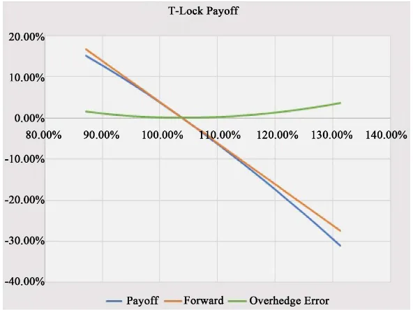
From (9), it can be seen that the payoff of a long Standard T-Lock struck at L may be approximated, at first order, by the t-value of a short forward contract struck at P Lte
( )
. Moreover, because the convexity of the T-Lock is negative in non-extreme scenarios away for the current yield as shown in Section 2.3, such forward contract constitutes a overhedge for the trade, as can be also observed from the joint plot in Figure 1, with respect to security price, for a 3-month T-Lock written on the 10Y benchmark as of 24 January 2019, i.e. Treasury, cou-pon 3.125%, maturity 25 November 2028 (ISIN US9128285M81). The spot in-ternal rate of return is 2.717% (Pmkt =104.1055, cleanprice 103.4922= ), the 3-months repo rate rrepo=2.46% , forward internal rate of returnIRR 2.53%= (forward dirty price 104.74%= ,forward clean price 103.36%= )
and L=2.717%.
The identification of such overhedge suggests that a short position on the T-Lock may be proxied by a long position on the forward contract on the same underlying and struck at
( )
e
t
K P L= (11)
( )
e e(
)
~ ForwardPricet t +RiskFactort ⋅ IRRt −L (12)
where:
DOI: 10.4236/jmf.2019.93018 305 Journal of Mathematical Finance
Figure 1. T-lock payoff and its overhedge.
RiskFactorte is the risk factor of the Security as computed at time te IRRt is the te-forward internal rate of return of the Security as computed
at time t, i.e., the rate such that
(
)
( )
e IRR ForwardPrice e
t t t
P = t (13)
at t t< e.
The forward contract proxy defined above may be regarded as a convenient representation of the Standard T-Lock in a practical situation where the T-Lock typology is not available in the trader’s front office risk management systems. In a later section we will analyse the risk generated by such approximation under standard mathematical assumptions that will make the treatment easier.
Because the security is not determined at inception, for the booking of the Then-Current-T-Lock a further issue arises. A natural extension is booking a Then-Current-T-Lock as a forward contract on the on-the-run benchmark as seen at inception and revise the booking each time a new on-the-run is taken over so that at te the proxy contract will match the real payout to the Client. Thus, for the purpose of investigating the pricing of a Then-Current-T-Lock, we turn our attention to the effect of replacing the security in the proxy forward contract.
Switching underlying security will lead to a new strike
( )
e
ˆ ˆt
K P L= (14)
with a strike gap, at first order,
ˆ
StrikeGap= −K K (15)
( )
( )
(
)
(
)
e e
e e
ˆForwardPrice ForwardPrice
ˆ ˆ
RiskFactor IRR RiskFactor IRR
t t
t t t t
t t
L L
= −
DOI: 10.4236/jmf.2019.93018 306 Journal of Mathematical Finance We can see that, ignoring the jump in RiskFactor, a reasonable assumption if the switch is actually a benchmark replacement within the same tenor (e.g. 10Y) or within close-”in-the-run” bonds, the strike gap reads
( )
( )
(
)
e
e e
ˆ
StrikeGap ForwardPrice ForwardPrice ˆ
RiskFactor IRR IRR
t t
t t t
t t
= −
+ ⋅ − (17)
The intuition is that the StrikeGap will generally be small if the switch is within close-”on-the-run” bonds but we will focus on this issue later in Section 3.1 turning our attention to a more meaningful measure, the P & L of the proxy forward contract.
From now on we will use Euler’s notation
( )
k( )
k
x k
f x f x
x ∂ ≡
∂
for high-order differentials.
2. Hedging the Standard T-Lock
In the current section we will look at the greeks (Hull [11], Chapter 19) generat-ed by a standard T-Lock position, bearing in mind though that the same results apply to the Then-Current-T-Lock in-between roll events. The first two subsec-tions are dedicated to the delta and gamma while in the third we touch on the practical implementation of the hedging strategy via the repo trade.
For ease of computation, we will assume the bond price to have the following functional form (Hull [11], Section 4.8, page 91], Taleb [12], page 184) with re-spect to the yield
( )
e(n ) e (i )i
n
t t y t t y
t i
t t
P y − − c α − −
>
= +
∑
(18)where c is the coupon rate of the bond and αi its accrual factors Under this assumption, with R the internal rate of return,
( )
y[ ]
y R(
)
g R = − ⋅a P = ⋅ R L− (19)
( )
( )
(
)
~a P L P R⋅ − (20)
( e) ( e)
e
mkt
e n e i
i
n
t t L t t L
i t t
a − − c α − − P
>
= ⋅ + −
∑
(21)Also, the first, second and third derivative of P y
( )
are easily computed, re-spectively, as[ ]
(
)
e (n )(
)
e(i )i
n
t t y t t y
y t n i i
t t
P t t − − c α t t − −
>
= − − −
∑
− (22)
which is a negative quantity (or null in limiting cases),
[ ]
(
)
2 ( )(
)
2 ( )2 e n e i ,
i
n
t t y t t y
y t n i i
t t
P t t − − c α t t − −
>
= − +
∑
− (23)
DOI: 10.4236/jmf.2019.93018 307 Journal of Mathematical Finance
[ ]
2
1
y P
P (24)
which is positive, and finally,
[ ]
(
)
3 ( )(
)
3 ( )3 e n e i
i
n
t t y t t y
y t n i i
t t
P t t − − c α t t − −
>
= − − −
∑
− (25)
which is negative.
As a consequence, the T-Lock payoff as a function of the yield
( )
y[ ]
(
)
g y = − ⋅a P y L⋅ − (26)
has first and second derivative, respectively,
[ ]
[ ]
(
)
y g = − ⋅a ∂∂ y y P y L⋅ −
(27)
[ ]
(
)
[ ]
2
y y
a P y L P
= − ⋅ ⋅ − + (28)
and
[ ]
[ ]
(
)
[ ]
2 3 2 2
y g = − ⋅a y P ⋅ y L− + y P
(29)
2.1. The Overhedge Error
We’re now in the position of being able to evaluate the accuracy of approxima-tion (9) which, looking at it backward, boils down to substituting P with its first order Taylor polynomial. The approximation is a (global) overhedge because the remainder
( )
( )
( )
1[ ]
(
)
1 y
R y =P y P L− − P y L− (30)
has a unique stationary point at y L= which is also a maximum, since the
second derivative of R y1
( )
is negative.Moreover, recalling the Remainder Estimation Theorem (see Apostol [13]) which states that, for a differential function P and all y in an interval I containing a point a, the error in using the Taylor polynomial of degree n to approximate P satisfies
( )
(
)
11 !
n
n
M y a R y
n
+ − ≤
+ (31)
where M is the maximum value of n1
[ ]
y+ P
in the interval I, for n=1, a L= we have that
( )
21 2
M y L
R y ≤ − (32)
where, because the third derivative of P (that is, the first derivative of 2
[ ]
y P
),
is negative, 2
[ ]
(
min)
yM = P I is taken to be the value at the left-most point of
the interval which is roughly (taking the extreme case y=0)
(
)
2(
)
2i
n
n i i
t t
t t c t t α
>
− +
∑
− (33)DOI: 10.4236/jmf.2019.93018 308 Journal of Mathematical Finance
~ 150
M (34) if we exclude the possibility of negative yields, an event that has never occurred (minimum yield for the 1Y Constant Maturity Treasury is 0.08% attained in September 2011). If we assume a 30% yield change, which is an upper bound for a short term such as 6 months for the 10Y benchmark, the dollar error amounts to 0.005% on 100% of notional.
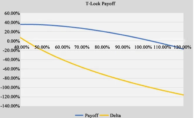
2.2. Delta of the T-Lock
Thanks to the smoothness of P y
( )
the greeks can be obtained by interchang-ing expected value and differentiation so for an analysis of delta and gamma of the T-Lock we will just look at the first and second derivatives of the payoff. From (28), when a=1, for y L− small enough (which is a reasonableas-sumption with short term expiries under typical business conditions),
[ ]
0y g >
(35)
so that the delta of the (long) T-Lock is negative
[ ]
[ ]
[ ]
0P g = y g ⋅ P y <
(36)
which is consistent with the previous comment about T-Lock being equivalent to shorting the security.
More precisely, resolving (28) for L, when a=1
[ ]
0 and 0 iff 2y[ ]
[ ]
y
y
P
g L y
P
> ∆ < > +
(37)
hence, because of the sign of the derivatives, we have a sharp lower bound smaller than y.
Turning things around
[ ]
0 and 0 iff 2[ ]
[ ]
0y y
y
P
g y L
P
> ∆ < − < − >
(38)
so, at least intuitively because the RHS of the inequality is also a function of y, as long as y does not overshoot L, the delta remains negative.
Taking into account the discounting, a trader, after booking the T-Lock posi-tion via proxy forward as argued in Secposi-tion 1.3, may delta hedge a short posiposi-tion via shorting an amount of bond equal to
[ ]
e ~Dtt P g
∆ (39)
and continuously re-adjust the hedge as market and time move. So the question is how trading the delta will affect the bank’s P & L, so we turn our attention to the gamma.
2.3. Gamma of the T-Lock
DOI: 10.4236/jmf.2019.93018 309 Journal of Mathematical Finance
[ ]
[ ]
[ ]
2[ ]
[ ]
2 2 2
P g = y g ⋅ P y + y g ⋅ P y
(40)
[ ]
[ ]
2[ ]
[ ]
(
[ ]
)
32 1 2
y g y P y g y P y P
= ⋅ − ⋅ (41)
From (28) and (29), the gamma of the T-Lock locally, i.e., y L− small
enough, satifies
[ ]
[ ]
[ ]
2[ ]
[ ]
(
[ ]
)
32 ~ 2 2 1 2
P g − ⋅a y P ⋅ y P + ⋅a y P ⋅ y P y P
[ ]
[ ]
2[ ]
(
[ ]
)
22 2
2 y 1 y y y
a P P a P P
= − ⋅ ⋅ + ⋅ (42)
[ ]
[ ]
22 1
y y
a P P
= − ⋅ ⋅ (43)
So, when a=1, with y L− small enough, the Gamma is negative (i.e., the
convexity of the T-Lock is negative), so dynamically replicating a T-Lock will, (not so) locally around L, generate rebalancing profits. In other words, dynami-cally replicating a long T-Lock via (10) and its delta assuming no volatility will be a overhedge, hence generating a non-negative P & L for the trader (see Carr and Madan [14], Equation (9)). More precisely, using (41), we see that
(
)
(
2[ ]
)
2[ ]
3[ ]
[ ]
2[ ]
0 iff y L y P y P y P y P y P
Γ < − ⋅ − ⋅ > ⋅
(44)
The latter factor satisfies
[ ]
(
2)
2[ ]
3[ ]
0
y P − y P ⋅ y P <
(45)
Proof. Thanks to (87) (Appendix C), noting that the leading summands ( )
(
0)
2 2yP
and 1 ( )0 3 ( )0
yP yP
− ⋅ cancel each other, we see that
[ ]
(
)
[ ]
[ ]
( )[ ]
(
)
(
( )[ ]
)
(
( )[ ]
)
2 2 3 20 0 0
2 2 3 3
y y y
y y y y y y
P P P
P c A P c A P c A
− ⋅
= + + + ⋅ +
(46)
( )
[ ]
( )[ ]
( )[ ]
[ ]
(
)
[ ]
[ ]
0 0 0
2 2 1 3 3 1
2
2 2 1 3
2
0
y y y y y y
y t y t y t
c P A P A P A
c A A A
= − −
+ − ⋅ <
(47)
This is because both summands are negative (from (88) and (89)) and the fact that c>0.
Finally, (44) and (45) yield
[ ]
[ ]
[ ]
(
)
[ ]
[ ]
2 2 2 30 iff y y 0
y y y
P P
y L
P P P
⋅
Γ < − < >
− ⋅
(48)
DOI: 10.4236/jmf.2019.93018 310 Journal of Mathematical Finance
Figure 2. T-lock delta.
Figure 3. T-lock gamma.
2.4. Replication of the T-Lock via Repo
[image:10.595.208.539.287.507.2]DOI: 10.4236/jmf.2019.93018 311 Journal of Mathematical Finance
( )
(
e(
)
)
(
e(
)
)
e
mkt repo repo
e e e
ForwardPrice 1 1 i
i
t t tt i t t i
t t t
t P r t t c α r t t
< ≤
= + − −
∑
+ − (49)where repo uv
r is the (simply compounded) forward repo rate for the period
u→v. We assume a zero haircut, which is a good approximation given the cre-dit quality of the Treasury.
Due to (49), (13) and (22), since by the chain rule and assuming a flat short-term repo curve,
( )
repo( )
( )
( )
reporepo repo
ForwardPrice
ForwardPrice
t t
y R P
g r g y y P r
y P
r = = r
∂ ∂ ∂ ∂
= ⋅ ⋅
∂ ∂
∂ ∂ (50)
the sensitivity of the T-Lock to the repo rate is negative, so the higher the repo rate the cheaper is the long position.
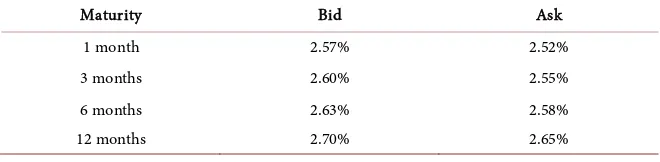
The typical bid-ask spread for a repo transaction is 5 basis points. For instance, as of 24 Jan 2019, we report the repo curve in Table 1 for GC (General Collateral) which shows positive repo rates for all tenors but, since the security is normally chosen to be a benchmark Treasury, a specialness (negative) premium may ap-ply so the repo rate may be significantly lower, increasing the fair value of the T-Lock position. Historically, in times of liquidity squeeze, the specialness has seen the repo rate on the 10Y Treasury momentarily drop into the negative axis at minus three hundred basis points (see Leong [16]).
In passing, it’s also interesting to note that given the current regime in the EUR market, being repo rates in the negative space, a hypothetical T-Lock writ-ten on a European treasury bond would be more expensive relative to a tradi-tional trade on a US Treasury.
3. Trading the Then-Current-T-Lock
As already represented in Section 1.3, in a Then-Current-T-Lock the underlying security is determined at te as the currently on-the-run benchmark. In the spe-cial and idealized case where te is coincides with the issue date of the new benchmark, the value at t t< e of a long(short) Then-Current-T-Lock struck at L is proxied by a short (long) forward contract struck at
(
)
e 1 RiskFactort t
K= + ⋅ R L− (51)
where
RiskFactorte is that of the Proxy Security as computed at time te
[image:11.595.209.539.647.728.2] Rt is the te-forward internal rate of return of the Proxy Security as com-puted at time t (see Equation (13))
Table 1. Repo rates for the 10Y as of 24 Jan 2019.
Maturity Bid Ask
1 month 2.57% 2.52%
3 months 2.60% 2.55%
6 months 2.63% 2.58%
DOI: 10.4236/jmf.2019.93018 312 Journal of Mathematical Finance Proxy Security is a traded security chosen in lieu of the yet unknown
under-lying, e.g., the on-the-run security as determined at time t.
At troll the new security must be selected and a new strike populated, the strike gap being
(
)
(
)
(
) (
)
(
)
e roll e roll
e e roll
e roll roll
ˆ ˆ
StrikeGap RiskFactor RiskFactor
ˆ ˆ
RiskFactor RiskFactor
ˆ RiskFactor
t t t t
t t t
t t t
R L R L
R L R R
= ⋅ − − ⋅ −
= − ⋅ −
− ⋅ −
(52)
In practice such a coincidence does not hold and because at inception the un-derlying security may be unknown and definitely not listed or identifiable in the position keeping system, the trader, via the procedure described in Section 1.3, may book the trade approximating the Then-Current-T-Lock as a Standard T-Lock with underlying security specified as the security that is on-the-run at trade inception. At each benchmark roll date troll, the booking is revised with the on-the-run at troll benchmark, generating a switch P & L, the roll P & L.
We will show in the approximated derivation (66) that the roll P & L must be small in special conditions. This is all the more the case at a on-the-run succes-sion, i.e., when the security rolls from the previous on-the-run benchmark to the new on-the-run issue. Indeed, the new on-the-run will normally have an internal rate of return in line with the existing level and, if we also take into account that because of the high frequency of issue (e.g. trimestral for the 10Y) the on-the-run succession normally brings a new coupon that is very close to that of the previous on-the-run, the roll P & L is potentially even less significant.
3.1. The Roll P & L
In this section we will present an approximated formula for the Roll P & L that will allow us, in the conclusive part of the paper, to compute statistical estimates.
To keep things simple, assume the security is switched from a bond with cou-pon rate c to a bond with coucou-pon rate cˆ, all other details remaining equal. The net present value changes from
( )
e e
t Dtt K F tt
π = − (53)
to
( )
e ˆ ˆ e
ˆt Dtt K F tt
π = − (54)
The P & L due to the switch is
(
)
(
( )
( )
)
e ˆ ˆ e e
ˆt t Dtt K K F tt F tt
π π− = − − −
(55)
with K P L= te
( )
, K P Lˆ = ˆte( )
and( )
( ) ( )ˆ e n ˆ e i
i
n
t t y t t y
t i
t t
P y − − c α − −
>
= +
∑
(56)DOI: 10.4236/jmf.2019.93018 313 Journal of Mathematical Finance
(
)
( e)e
ˆ ˆ e i
i
n
t t L i t t
K K c c α − −
>
− = −
∑
(57)Now, by definition
( )
e e( )
t t t
F t =P R (58)
and
( )
e e( )
ˆ ˆ ˆ
t t t
F t =P R (59)
therefore
( )
e( )
e e( )
e( )
ˆ ˆ ˆ
t t t t t t
F t −F t =P R −P R (60)
( ) ( )
( )
( )
e e e e
ˆ ˆt t t ˆt t ˆt t t
P R P R P R P R
= − + − (61)
(
)
( e)( )
( )
e e
e
ˆ ˆ
ˆ e i t
i
n
t t R
i t t t t
t t
c c α − − P R P R
>
= −
∑
+ − (62)where, when t tn− e is small, i.e., the bond at te is close to the bond’s maturity, the last summand
( )
( )
( e) ( e)e e
ˆ
ˆ e t t Rn t e t t Rn t
t t t t
P R −P R = − − − − − (63)
( ) ( )
(
e e)
eˆ
e i t e i t
i
n
t t R t t R
i t t
c α − − − −
>
+
∑
− (64)can be approximated, at first order, as
( )
( ) (
)
(
)
(
)
e e
e
e e
ˆ ~ ˆ
i
n
t t t t n i i t t
t t
P R P R t t c α t t R R
>
− − + − −
∑
(65)so that the (forward) P & L satisfies
(
)
( e) ( e)e e
e
ˆ
ˆ ˆ
e i e i t
i i
n n
t t L t t R
t t
i i
t t t t
tt
c c D
π π α − − α − −
> >
−
= − −
∑
∑
(66)( )
( )
e ˆ e
t t t t
P R P R
− − (67)
(
)
( e) ( e)e e
ˆ
ˆ
~ e i e i t
i i
n n
t t L t t R
i i
t t t t
c c α − − α − −
> >
− −
∑
∑
(68)(
)
(
)
(
)
e e e ˆ i nt t n i i
t t
R R t t c α t t
>
+ − − + −
∑
(69)(
)
(
)
(
)
e e ˆ ˆ ~ i nt i i
t t
c c R L α t t
>
− −
∑
− (70)(
)
(
)
(
)
e e e ˆ i nt t n i i
t t
R R t t c α t t
>
+ − − + −
∑
(71)Similarly, it can be shown that
(
)(
)
(
)
e e e ˆ ˆ ~ i n t tt i i
t t tt
c c L R t t
D
π π α
>
− − − −
DOI: 10.4236/jmf.2019.93018 314 Journal of Mathematical Finance
(
)
(
)
(
)
e
e e
ˆ ˆ
i
n
t t n i i
t t
R R t t c α t t
>
+ − − + −
∑
(73)Therefore, in as a much as t tn− e is small
L is close to Rt
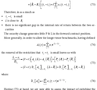
there is no significant gap in the internal rate of return between the two se-curities
The security change generates little P & L in the forward contract position. More generally, in order to allow for longer tenor benchmarks, having defined
( )
e (i ) ,i
n
t t y
t i
t t
A y α − −
>
=
∑
(74)the removal of the restriction that t tn− e is small leaves us with
(
)
( )
( )
( )
( )
(
)
(
)
(
)
e e e e
e
e ˆ e ˆ
ˆ ˆ ˆ ˆ
ˆ ˆ
ˆ ~
t t
t t
t t t t t t t
tt
y t y R t y t y R t t
c c A L A R P R P R D
c c A L R P R R
π π
= =
−
= − − + −
− ⋅ ⋅ − + ⋅ −
(75)
where
[ ]
(
)
e(i ) ,i
n
t t y
y t i i
t t
A α t t − −
>
= −
∑
− (76)
Having (75) at hand, we are now able to assess the impact of switching the underlying security of the contract at the issue of a new benchmark. To this aim, in the next section we will look at a stylized description of how a new benchmark is constructed, where we ignore the change in the tenor structure of the bond, only focusing on the determination of a new par coupon rate so that the new benchmark is priced at par.
3.2. Forming the New Benchmark
Treasury benchmarks are periodically reissued by means of an auction mechan-ism. The US government yearly publishes an auction calendar ([17]).
The roll process is described in the graph (Figure 4), where the bracketed ex-ponent on P( ) is a placeholder for the coupon rate, a process that runs as
fol-lows:
First the internal rate of return Rt of the current benchmark is evaluated The prospected coupon cˆ of the new benchmark is located so that the new
issue is at par, i.e., ( )cˆ
( )
1t t
P R =
Then the auction will filter through market appetite determining a final coupon rate cˆ′
Finally, the new internal rate of return Rˆt is implied from ( )cˆ
( )
ˆt t
[image:14.595.202.544.71.389.2]P ′ R .
DOI: 10.4236/jmf.2019.93018 315 Journal of Mathematical Finance It’s clear that if the market confirms the new issue “at the old level” we land on R Rˆt = t so, as can be elicited from Equation (75), minimizing the roll P & L.
Because the above assumptions are normally not verified, to estimate the roll risk in practice, in Section 4.3 we will resort to a statistical analysis based on the history of auctions.
4. Statistical Analysis
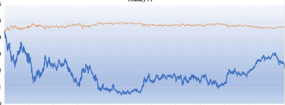
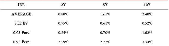
[image:15.595.66.530.271.453.2]Looking at market data from January 2008 for the 2Y, 5Y and 10Y Treasury benchmark (see Figures 5-7), we have the following summary statistics in Table 2. The summary shows the average, the standard deviation and the two classic percentiles of the sample. Note that, in order to encompass non-standard scena-rios, the data set includes the 2007 crisis.
Figure 5. Treasury 2Y: Internal rate of return and risk factor.
[image:15.595.69.535.515.688.2]DOI: 10.4236/jmf.2019.93018 316 Journal of Mathematical Finance
Figure 7. Treasury 10Y: Internal rate of return and risk factor.
Table 2. Treasuries: Internal rate of return statistics.
IRR 2Y 5Y 10Y
AVERAGE 0.88% 1.61% 2.40%
STDEV 0.75% 0.61% 0.52%
0.05 Perc 0.24% 0.70% 1.62%
0.95 Perc 2.59% 2.77% 3.34%
In the following sections we will use such historical data to verify in practice our guess regarding the efficacy of managing the risk generated by short T-Lock positions by booking them as forward contracts. The statistical anaysis is aimed at estimating:
1) The overhedge error (Section 4.1) due to the payoff approximation illu-strated in Section 1.3.
2) The gamma negativity bounds (Section 4.2), that is the stability of negative sign of the gamma across market scenarios.
3) The roll risk (Section 4.3) due to the P & L of the Bank generated during the life of the contract by the mispecification and consequent revision of the se-curity underlying the sold T-Lock.
4.1. Overhedge Error Estimation
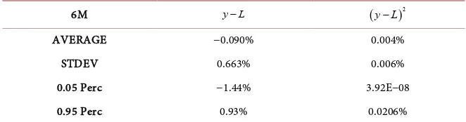
We first look at the overhedge error (9) by extracting a historical estimation for (32). Considering a 6M T-Lock on the 10Y benchmark, we find (Table 3) that
2
[image:16.595.209.540.327.418.2]DOI: 10.4236/jmf.2019.93018 317 Journal of Mathematical Finance
Table 3. Overhedge error.
6M y L− ( )2
y L−
AVERAGE −0.090% 0.004%
STDEV 0.663% 0.006%
0.05 Perc −1.44% 3.92E−08
0.95 Perc 0.93% 0.0206%
downgrade by the major rating agencies (Brandimarte and Bases [18]). For the estimations in Table 3 we have assumed to be in a typical business case where the locked yield L to be set at the IRR seen at inception t, so that y L− is taken
to be the 6-month performance Rt+6M−Rt of the IRR. For ease of reading we omit reporting estimates for other cases, such as 3M, yielding similar results.
4.2. Negative Gamma Bounds
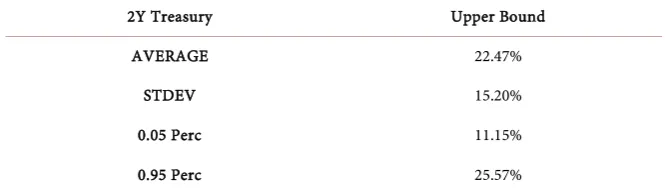
Considering the same historical window, in the following we have considered a daily time series of the upper bound (48) and reported in Tables 4-6 the relevant statistics. A move of such magnitude within the typical features (expiry and at-the-money strike) of a T-Lock trade is highly unlikely and has never been recorded being outside ordinary levels of core governative yields.
4.3. Assessment of the Roll Risk
We have considered roll data from January 2008 for the 10Y Treasury bench-mark. It is a very large time window which is chosen to encompass extreme his-torical scenarios.
From Table 7, we see that, for the 10Y, the IRR change at roll dates tends to be higher than the IRR change on the whole sample. Consequently we expect P & L change an unfavourable on the T-Lock position at each benchmark switch.
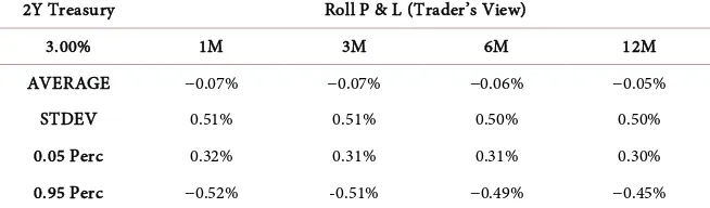
To further the analysis, in the following we will look at the statistics regarding the actual P & L. Ignoring the discounting effect, which is a reasonable approxi-mation by virtue of the short time horizon under scrutiny, we have considered a time series of (75) and computed the relevant percentiles and value-at-risk for the (forward) net present value of the forward contract for 1M, 3M, 6M, 12M expiries and 3% locked yield. From the point of view of the trader selling the T-Lock on the 10Y (Table 8): the average roll generates for the trader roughly a −0.105% of the notional loss which peaks at −1.04% at the 95-th percentile for the shortest expiry.
DOI: 10.4236/jmf.2019.93018 318 Journal of Mathematical Finance
Table 4. Upper bound for negative gamma for the 10Y.
10Y Treasury Upper Bound
AVERAGE 11.44%
STDEV 0.10%
0.05 Perc 11.28%
[image:18.595.210.539.223.320.2]0.95 Perc 11.61%
Table 5. Upper bound for negative gamma for the 5Y.
5Y Treasury Upper Bound
AVERAGE 21.31%
STDEV 0.12%
0.05 Perc 21.11%
[image:18.595.207.540.355.450.2]0.95 Perc 21.51%
Table 6. Upper bound for negative gamma for the 2Y.
2Y Treasury Upper Bound
AVERAGE 22.47%
STDEV 15.20%
0.05 Perc 11.15%
0.95 Perc 25.57%
Table 7. Treasury 10Y: Yield change.
10Y Treasury Yield Change Yield Change on Roll
AVERAGE −0.0006% 0.0123%
STDEV 0.0497% 0.0571%
0.05 Perc −0.0760% −0.0528%
0.95 Perc 0.0794% 0.1166%
Table 8. Roll P & L for the 10Y.
10Y Treasury Roll P & L (Trader’s View)
3.00% 1M 3M 6M 12M
AVERAGE −0.1085% −0.1069% −0.1045% −0.0996%
STDEV 0.5028% 0.4953% 0.4841% 0.4615%
0.05 Perc 0.4749% 0.4677% 0.4568% 0.4352%
[image:18.595.212.540.488.579.2] [image:18.595.211.542.614.726.2]DOI: 10.4236/jmf.2019.93018 319 Journal of Mathematical Finance
Table 9. Roll P & L for the 5Y.
5Y Treasury Roll P & L (Trader’s View)
3.00% 1M 3M 6M 12M
AVERAGE −0.05% −0.04% −0.04% −0.04%
STDEV 0.22% 0.22% 0.21% 0.18%
0.05 Perc 0.24% 0.23% 0.22% 0.20%
0.95 Perc −0.43% −0.42% −0.40% −0.35%
Table 10. Roll P & L for the 2Y.
2Y Treasury Roll P & L (Trader’s View)
3.00% 1M 3M 6M 12M
AVERAGE −0.07% −0.07% −0.06% −0.05%
STDEV 0.51% 0.51% 0.50% 0.50%
0.05 Perc 0.32% 0.31% 0.31% 0.30%
0.95 Perc −0.52% -0.51% −0.49% −0.45%
5. Valuation Adjustments
Just as any derivative, a position on the T-Lock carries counterparty risk (see Gregory [19], Morini and Prampolini [20]). As such, CVA and DVA should also be included in the book value of the trade and in the final price to the client.
The calculation of such adjustments is a run-of-the-mill task for a bank deal-ing in derivatives but, whereas it may be argued that short-term trades generally attract low counterparty risk, we also notice that a T-Lock short position is sub-ject to systemic wrong-way counterparty risk. Indeed, on a distressed scenario where the corporate market is undermined, a flight-to-quality ensuing regime may concurrently lower the Treasury spreads increasing the Bank exposure to the Client. It is difficult though to envision a situation where the corporate sec-tor suffers and the banks thrive so it may be argued that the adverse move of the CVA may be offset by a specular increase in the DVA component, lowering the potential impact of wrong-way-risk on the bank’s balance sheet.
As for the FVA (Andresen, Duffie and Song [21], Morini and Prampolini [20], Albanese and Andreasen [22]), having noticed that the natural hedge is a repo trade, a funding cost arises from the cash leg of the hedge the Bank is posting to borrow the security or from the collateralization mechanism if the repo is CSA-assisted or cleared.
From the point of view of the dealer bank, capital costs (KVA) are also mi-nimal allowing for a interesting profitability of T-Locks although, by the same token, the trade will not afford high mark-ups.
[image:19.595.211.538.228.324.2]Al-DOI: 10.4236/jmf.2019.93018 320 Journal of Mathematical Finance banese and Andreasen [22]) of counterparty risk, funding value adjustments and KVA. Nevertheless the short-term nature of the transaction under investigation will mitigate the consequences of such underestimation considering that XVA’s for at-the-money trades are normally priced at a fraction of the carried exposure.
6. Conclusions
We have shown that a long Standard T-Lock position has negative convexity, so the trader may safely (over-)replicate it by booking a linear trade, a proxy for-ward contract, which is a natural overhedge. In other words, a trader willing to sell a Standard T-Lock position can book the trade as a forward contract written on the same security and with the same expiry as that of the T-Lock contract. Being an overhedge, the forward contract will generate a conservative represtation of bank’s P & L associated to the position. The negative convexity will en-sure that delta hedging the positions will generate gamma profits. This comes in handy when the front office risk management system does not feature the T-Lock as a typology.
Moreover, we have shown that a T-Lock position is historically little sensitive to the benchmark roll. Therefore, a trader may book a Then-Current-T-Lock trade as a proxy forward contract written on the security that is on-the-run benchmark at inception and remain confident that revising the booking at roll dates to update the underlying will statistically generate a negligible P & L, while again, thanks to the negative convexity of the T-Lock, delta hedging the position in between roll dates will generate gamma profits.
Conflicts of Interest
The author declares no conflicts of interest regarding the publication of this pa-per.
References
[1] The PNC Financial Services Group (2019) Hedging Future Bond Issuance. https://www.pnc.com/en/corporate-and-institutional/financing/lending-options/pn c-real-estate/News-Articles-and-Transaction-Spotlights/REArticles/how-to-hedge-f
uture-bond-issuance.html
[2] Valtchev, Y. (2015) Corporate Treasury Risk Management.
http://financedocbox.com/Options/75981452-Corporate-treasury-risk-management .html
[3] Bank of Montreal (1997) Locking in Treasury Rates with Treasury Locks.
https://www.bmocm.com/common/scripts/getfile.aspx?fileID=67
[4] US Securities and Exchange Commission (2005) Eight Treasury Rate Lock Agree-ments.
https://www.sec.gov/Archives/edgar/data/31978/000119312505099245/dex1002.htm
[5] Adams, J. and Smith, D.J. (2011) Pre-Issuance Hedging of Fixed-Rate Debt. Journal of Applied Corporate Finance, 23, 102-112.
DOI: 10.4236/jmf.2019.93018 321 Journal of Mathematical Finance
[6] Ramirez, J. (2015) Accounting for Derivatives: Advanced Hedging under IFRS. Wi-ley, Hoboken.https://doi.org/10.1002/9781119065876
[7] PWC (2017) In Depth: Achieving Hedge Accounting in Practice under IFRS 9. [8] Hunt, P.J. and Kennedy, J.E. (2004) Financial Derivatives in Theory and Practice.
Wiley Series in Probability and Statistics, Hoboken.
https://doi.org/10.1002/0470863617
[9] EY (2014) Hedge Accounting under IFRS 9.
[10] Pucci, M. (2014) Constant Maturity Treasury Convexity Correction. International Journal of Theoretical and Applied Finance, 17, Article ID: 1450051.
https://doi.org/10.1142/S0219024914500514
[11] Hull, J.C. (2015) Options, Futures and Other Derivatives. Ninth Edition, Prentice Hall, Upper Saddle River.
[12] Taleb, N. (1996) Dynamic Hedging. John Wiley & Sons, Hoboken. [13] Tom, A. (1967) Calculus. Wiley, Hoboken.
[14] Carr, P. and Madan, D. (2002) Towards a Theory of Volatility Trading.
http://pricing.online.fr/docs/TradingVolatilityStrat.pdf
[15] ICMA Group (2015) Frequently Asked Questions on Repo.
http://www.icmagroup.org/Regulatory-Policy-and-Market-Practice/short-term-mar
kets/Repo-Markets/frequently-asked-questions-on-repo
[16] Leong, R. (2014) Bearish Bond Bets Send U.S. Repo Rates into the Red.
https://www.reuters.com/article/markets-usa-repos-idUSL2N0OR10J20140610
[17] U.S. Department of the Treasury (2019) Tentative Auction Schedule of U.S. Trea-sury Securities. https://www.treasurydirect.gov/instit/annceresult/press/press.htm [18] Brandimarte, W. and Bases, D. (2011) United States Loses Prized AAA Credit
Rat-ing from S&P. August 7, 2011.
[19] Jon, G. (2010) Counterparty Credit Risk. Wiley, Hoboken.
[20] Morini, M. and Prampolini, A. (2016) Risky Funding: A Unified Framework for Counterparty and Liquidity Charges. Landmarks in XVA.
[21] Andersen, L., Duffie, D. and Song, Y. (2019) Funding Value Adjustments. The Journal of Finance, 74, 145-192.https://doi.org/10.1111/jofi.12739
[22] Albanese, D., Andersen, L. and Iachibino, S. (2015) FVA Accounting, Risk Man-agement and Collateral Trading. Risk Magazine, January.
DOI: 10.4236/jmf.2019.93018 322 Journal of Mathematical Finance
Appendix
A. Simple Math
Below we recall simple facts about first and second derivatives of differentiable functions. If f and g are differentiable then
(
f g)
′= f g′ ′⋅ (77) and(
f g) (
′′= f′′ g) ( ) (
⋅ g′2+ f g g′)
⋅ ′′ (78)
As a consequence, if f invertible and differentiable then
( )
f 1 1f
− ′ =
′ (79)
and
( )
1( )
3f f
f
− ′′ = − ′′
′ (80)
B. Key Derivatives Noting that
( )c
( )
( )0( )
( )
,t t t
P y =P y cA y+ (81)
and
( )c
(
)
e(t t yn )[ ]
yPt = − tn−t − − +c y At
(82)
( )0
[ ]
yPt c y At
= + (83)
we can work out that
( )
(
)
e (n )(
)
e(i )i
n
k t t y k t t y
c k
y n i i
t t
P t t − − c α t t − −
>
= − + −
∑
(84)
[ ]
(
)
e (i ) ,i
n k
t t y k
y t i i
t t
A α t t − −
>
=
∑
− (85)
and
( )c
(
)
ke(t t yn )[ ]
k k
yPt = − t tn − − +c y At
(86)
( )0
[ ]
k k
yPt c y At
= + (87)
C. More Math
Setting
q
i= −
(
t t
i)
, Qi=α
ie− −(t t yi ) we see that( )0
[ ]
( )0[ ]
( )0[ ]
1 3 3 1 2 2 2 0
yPt y At + yPt y At − yPt y At ≥
(88)
because
[
]
23 3 2 2
i i i i
n n i i n n i i n n i i i n i n i n
t t t t t t t t
q Q q Q q Q q Q q Q q Q Q Q q q q q
> > > >
+ − = −
∑
∑
∑
∑
DOI: 10.4236/jmf.2019.93018 323 Journal of Mathematical Finance
[ ]
(
2)
2 1[ ]
3[ ]
0
y At − y At ⋅ y At <
(89)
because
2
2
3 2
, 0
i i i i j
i i i i i i i j i j
t t> q Q t t> q Q t t> q Q t t t t> >Q Q q q
− = − >
∑
∑
∑
∑
(90)Indeed,
2
3 2 3 2 2
i i i
i i i i i i i j i j i j i j
t t t t t t i j i j
q Q q Q q Q q q Q Q q q Q Q
> > > ≠ ≠
− = −
∑
∑
∑
∑
∑
(91)(
3 3)
2 2 2i j i j i j i j i j
i j i j
q q q q Q Q q q Q Q
< <
=
∑
+ −∑
(
3 3)
2 2 2i j i j i j i j i j
i j< q q q q Q Q q q Q Q
=
∑
+ − (92)(
2 2)
2 2 2i j i j i j i j i j
i j< q q q q Q Q q q Q Q
=
∑
+ − (93)(
)
2i j i j i j
i j< q q Q Q q q
=
∑
− (94)is clearly positive2.
D. The Forward Price and the Repo
A coupon security/dividend security X is a security that pays a discrete stream of cashflows ci, each at time Ti. It could be either a stock or a coupon bond.
If hcut is the haircut, the T-forward price of the security, paying a dividend i
c at time Ti, i=1, , n, is
( )
(
cut)
repo( ) cut fun( )ForwardPrice 1 er T t er T t
t T =Xt −h − +h − (95)
(
)
(
cut fun 1 cut repo)
( )< e
i i
h r h r T T
i
t T Tc
+ − −
≤
−
∑
(96)where rrepo is the repo rate, rfun is the funding rate for unsecured borrowing. Both rates are assumed continuously compounded and flat for ease of illustra-tion.
Assuming first hcut=0, in a repo trade with dividends/coupons with ma-turity T the trader
1) Borrows in the time interval
[
T T
0,
1]
an amount Xt of cash at rate rrepo until T, with which s/he buys bond from the market and immediately transfers it to the repo counterparty.2) Then for each
[
T T
i−1,
i]
on each bond schedule node Ti, receive coupon ic and decrease the borrowed outstanding in the repo by ci.
3) At T, s/he gets the bond back, sells it in the market and returns all out-standing borrowed cash to the repo counterparty.
We describe our position by the quantity At which represent the cash owned (plus sign)/owed (minus sign) to the repo counterparty, the repo account. 2For ease of reading, in the above summations we have omitted typing the conditions
i t t> and
DOI: 10.4236/jmf.2019.93018 324 Journal of Mathematical Finance At start on the repo trade our repo account amounts to At = −Xt. At each coupon payment we decrease the outstanding by the coupon amount. For in-stance, at T1 the repo account becomes
( )
repo 1
1 1 e
r T t
T t
A = +c A − (97)
Then, recursively, for i=2, , q, at Ti
( )
repo 1 1e
i i
i i
r T T
T i T
A c A −
−
−
= + (98)
and finally from Tq to T it accrues to the terminal value ( )
repo
er u Tq
u q
A =A − (99)
Working out the recursion we see the repo cash account grows as Lemma 1. For all u t≤ ,
( ) ( )
repo repo
e i e
i
r u T r u t
u i t
t T u
A c − X −
< ≤
=
∑
− (100)So at maturity the strategy is worth
T T T
v =X +A (101)
In other words, the trader enters at t a contract at zero cost and ends up, via the repo strategy, at T with a XT in exchange for AT, which means, by defini-tion, that AT is the T-forward price of the security
( )
repo( ) repo( )ForwardPrice e e i
i
r T T
r T t
t t i
t T T
T X − c −
< ≤
= −
∑
(102)If, on the other hand, due to market illiquidity the repo trade is not viable for the given security, the formula still holds but with rfun in lieu of rrepo
( )
fun( ) fun( )ForwardPrice e e i
i
r T T
r T t
t t i
t T T
T X − c −
< ≤
= −
∑
(103)The two cases (102), (103) are the extreme cases:
hcut =0: all funding is secured since based on the repo trade hcut =1: there is no repo trade, all funding is unsecured.
Finally, for a generic haircut 0≤hcut ≤1 we obtain a “blend” formula:
( )
(
cut)
repo( ) cut fun( )ForwardPrice 1 er T t er T t
t T Xt h h
− −
= − + (104)
(
)
(
cut fun 1 cut repo)
( )e i
i
h r h r T T
i
t T Tc
+ − −
< ≤
−