Transience and multifractal analysis

Accepted Manuscript

Transience and multifractal analysis

Godofredo Iommi, Thomas Jordan, Mike Todd

PII: S0294-1449(16)30001-4

DOI: http://dx.doi.org/10.1016/j.anihpc.2015.12.007 Reference: ANIHPC 2776

To appear in: Annales de l’Institut Henri Poincaré - Analyse non linéaire

Received date: 11 April 2015 Revised date: 25 September 2015 Accepted date: 15 December 2015

Please cite this article in press as: G. Iommi et al., Transience and multifractal analysis,Ann. I. H. Poincaré – AN(2016), http://dx.doi.org/10.1016/j.anihpc.2015.12.007

GODOFREDO IOMMI, THOMAS JORDAN, AND MIKE TODD

Abstract. We study dimension theory for dissipative dynamical systems, proving a conditional variational principle for the quotients of Birkhoff av-erages restricted to the recurrent part of the system. On the other hand, we show that when the whole system is considered (and not just its recurrent part) the conditional variational principle does not necessarily hold. Moreover, we exhibit an example of a topologically transitive map having discontinuous Lyapunov spectrum. The mechanism producing all these pathological features on the multifractal spectra is transience, that is, the non-recurrent part of the dynamics.

1. Introduction

The dimension theory of dynamical systems has received a great deal of atten-tion over the last fifteen years. Multifractal analysis is a sub-area of dimension theory devoted to study the complexity of level sets of invariant local quantities. Typical examples of these quantities are Birkhoff averages, Lyapunov exponents, local entropies and pointwise dimension. Usually, the geometry of the level sets is complicated and in order to quantify its size or complexity tools such as Hausdorff dimension or topological entropy are used. Thermodynamic formalism is, in most cases, the main technical device used in order to describe the various multifractal spectra. In this note we will be interested in multifractal analysis of Birkhoff av-erages and of quotients of Birkhoff avav-erages. That is, given a dynamical system T : X → X and functions φ, ψ :X →R, with ψ(x)>0, we will be interested in the level sets determined by the quotient of Birkhoff averages ofφwithψ. Let

α_m=α_m,φ,ψ:= inf

lim

n→∞

_n−1

i=0 φ(Tix) _n−1

i=0 ψ(Tix)

:x∈X

and (1)

αM =αM,φ,ψ:= sup

lim

n→∞

n−1

i=0 φ(Tix) n−1

i=0 ψ(Tix)

:x∈X

. (2)

Date: January 8, 2016.

G.I. was partially supported by the Center of Dynamical Systems and Related Fields c´odigo ACT1103 and by Proyecto Fondecyt 1150058. T.J. wishes to thank Proyecto Mecesup-0711 for funding his visit to PUC-Chile. M.T. is grateful for the support of Proyecto Fondecyt 1110040 for funding his visit to PUC-Chile and for partial support from NSF grant DMS 1109587. The authors thank the referees for their careful reading of the paper and useful suggestions.

For α ∈ [α_m, α_M] we define the level set of points having quotient of Birkhoff average equal toαby

J(α) =J_φ,ψ(α) :=

x∈X : lim

n→∞

_n−1

i=0 φ(Tix) _n−1

i=0 ψ(Tix) =α

. (3)

Note that these sets induce the so calledmultifractal decomposition of the repeller,

X =

αM

α=αm

J(α) ∪J,

whereJ is theirregular set defined by,

J=J_φ,ψ :=

x∈X : the limit lim

n→∞

n−1

i=0 φ(Tix) n−1

i=0 ψ(Tix)

does not exist

.

Themultifractal spectrum is the function that encodes this decomposition and it is defined by

b(α) =b_φ,ψ(α) := dim_H(J_φ,ψ(α)),

where dimH denotes the Hausdorff dimension (see Section 2.3 or [Fa] for more

details). Note that ifψ≡1 thenbφ,1gives a multifractal decomposition of Birkhoff averages. If the set X is a compact interval, the dynamical system is uniformly expanding with finitely many piecewise monotone branches and the potentials φ and ψ are H¨older, it turns out that the map α → b_φ,ψ(α) is very well behaved. Indeed, bothα_m,φ,ψandα_M,φ,ψ are finite and the mapα→b_φ,ψ(α) is real analytic (see the work of Barreira and Saussol [BS]).

In the case where eitherφ= log|T|orψ= log|T|the mapα→bφ,ψ(α) can often

be determined by looking at a Legendre or Fenchel transform of a suitable pressure function. In this case the results have been extended well beyond the uniformly hyperbolic setting, see [GR, HMU, I, KU, KS, FLWW, N, O, PoW, TV]. However without the assumption of uniform hyperbolicity it is no longer always the case thatα→bφ,ψ(α) will be analytic as shown in [GR, KMS, N, O, TV].

For more general functions φ and ψ the relationship to the Legendre or Fenchel transforms of certain pressure functions no longer holds. However in [BS] it is shown α → b_φ,ψ(α) can still be related to suitable pressure functions. Some of these results were extended by Iommi and Jordan [IJ2] to the case of expanding full-branched interval maps, with countably many branches. However, as already mentioned, in this situation it is not always the case that the spectrum is real analytic. In [IJ2] it is shown that there will be regions where the spectrum does vary analytically but the transitions between these regions may not be analytic or even continuous. In the situation where the map is non-uniformly expanding, for example the Manneville-Pomeau map, it was shown in [GR, O, N, TV] that the Lyapunov spectrum (equivalently the local dimension spectrum for the measure for maximal entropy) has a phase transition. In the general case the spectrum may be related to those studied in [IJ2]. In this case it will not always be continuous, see Section 6 of [IJ2]. The lack of uniform hyperbolicity of the dynamical system being the reason for the irregular behaviour of the multifractal spectrum.

of dynamical systems (not necessarily uniformly hyperbolic) and for a large class of potentials (not necessarily H¨older) that the following holds:

b_φ,ψ(α) = sup

h(μ)

log|F|dμ :

φdμ

ψdμ =αandμ∈ M

,

whereMdenotes the set ofT−invariant probability measures. See [BS, Cl, FFW, FLP, FLW, H, IJ1, JJOP, Ol, PW] for works where this conditional variational principle has been obtained with different degrees of generality.

The aim of the present paper is to study multifractal spectra of quotients of Birkhoff averages when the map is modelled by a topologically mixing countable Markov shift with no additional assumptions (e.g. the incidence matrix is not assumed to be finitely primitive). This allows us to study certain dissipative maps by which we mean maps where the Hausdorff dimension of the set of recurrent points is smaller than the Hausdorff dimension of the repeller of the map (see Sections 2.2 and 2.3 for precise definitions). Note that in this situation we cannot use the techniques from [IJ1] and [IJ2] since both these papers are restricted to maps which can be modelled by a full shift (under this assumption the thermodynamic formalism is very well behaved and understood [Sa2]) and the techniques can not be applied without additional assumptions on the incidence matrix.

The multifractal analysis for the local dimension of Gibbs measures in this setting has been studied in [I] but the technique of inducing used there does not work so well in the setting of Birkhoff averages and so we take a different approach. Let us point out that dimension spectra of quotients of Birkhoff averages has been studied in the particular case in which ψ = log|T| in the work of Barreira, Saussol and Schmeling [BSSc] for uniformly hyperbolic systems defined over compact spaces and by Kesseb¨ohmer and Urba´nski [KU] for maps that can be coded by countable Markov shifts with finitely primitive incidence matrix. In both cases there exist Gibbs measures for sufficiently smooth potentials [MU] which provides a powerful tool which simplifies the proofs. We stress that if the countable Markov shift does not have an finitely primitive incidence matrix then smooth potentials do not have corresponding Gibbs measures [Sa3].

In this paper we exhibit some of the pathologies that can easily occur in the di-mension theory of dissipative systems. We not only study the didi-mension of the conservative part of the system but also the multifractal decomposition of the whole repeller (see Section 4). The example to which we will devote more attention is a model for an induced map of a Fibonacci unimodal map (see Section 4) which has been studied by Stratmann and Vogt [SV] and by Bruin and Todd (see [BT1, BT2]).

We prove that the conditional variational principle for quotients of Birkhoff averages holds under certain assumptions when restricted to the recurrent set. Moreover, we exhibit a map for which the Birkhoff spectrum b(α) is discontinuous. In this example the mechanism producing the discontinuity is transience. Note that the Birkhoff spectrum for this map does not satisfy the conditional variational principle for certain H¨older potentials. We stress that while recently in [IJ2] examples of discontinuous Birkhoff spectra were found in the non-uniformly hyperbolic setting, the situation we treat here is of a completely different nature.

The study of transience in dynamical systems has attracted some attention recently and its implications in thermodynamic formalism has been explored (see [C, CS, IT, Sa2]). In this note we study some of the consequences that transience has in dimension theory. Of particular interest is Proposition 4.4 where we exhibit a map having discontinuous Lyapunov spectrum. This particular case of Birkhoff spectrum has been thoroughly studied over the last years in a wide range of contexts. Examples have been found where it is not a real analytic map (see [GR, N]). In other cases the domain of the spectrum is not an interval. Indeed, the Chebyshev mapT(x) = 4x(1−x) defined on the unit interval has only two Lyapunov exponents and hence the domain of the Lyapunov spectrum consists of two isolated points. More generally, Makarov and Smirnov [MS] showed that there are rational mapsT for which the domain of the Lyapunov spectrum consists of an interval together with finitely many isolated points. However, the dimension of the set of points having Lyapunov exponent equal to one of these isolated points is zero. The example we provide goes in the exact opposite direction. The domain is an interval but at the largest point in the domain the Hasudorff dimension jumps to 1.

2. Notation and statement of our main result

This section is devoted to stating the conditional variational principle for the quo-tient of Birkhoff averages restricted to the recurrent set, followed by some prelimi-nary results we will need to prove it. In order to do this, we will define the class of maps and potentials that we will consider as well as to recall some basic definitions from geometric measure theory.

2.1. Symbolic spaces. Let (Σ, σ) be a one-sided Markov shift over the countable alphabetN. This means that there exists a matrix (t_ij)_N×Nof zeros and ones (with no row and no column made entirely of zeros) such that

Σ := (xn)n∈N:txixi+1= 1 for everyi∈N

.

that for every a, b ∈N there exists a positive integer N such that for all n ≥N there exists an admissible wordaof lengthnsuch thata0=aanda_n−1=b. Unlike the finite state case, this does not imply that some power of the transition matrix is positive. The space Σ endowed with the topology generated by the cylinder sets

Ci1i2...in :={(xn)∈Σ :xj =ij forj∈ {1,2,3. . . n}},

is a non-compact space. We define then-th variation of a functionφ: Σ→Rby

varn(φ) = sup

(i1...in)_∈Nn_x,y∈Csup_i1i2...in|φ(x)−φ(y)|.

A function φ: Σ→Ris locally H¨older if there exists 0< γ <1 andC >0 such that for everyn∈Nwe havevar_n(φ)≤Cγn _{(note that this condition allowsφto}

be unbounded).

2.2. The class of maps. Given a compact intervalX ⊂R, let{X_n}_n⊂X be a countable collection of disjoint subintervals and letT :∪_nX_n→X be a map which is differentiable on the interior of each setX_n. Therepeller of the mapT is defined by

X∞:={x∈X :Tn_{(x) is defined for alln∈N}.}

We say that the map T is Markov if there exists a countable Markov shift (Σ, σ) and a continuous bijective mapπ: Σ→X∞such thatT◦π=π◦σ. We will use the notation [i1, . . . , in] :=π(Ci1...in). LetRdenote the set of potentialsφ:∪nXn→R

such thatφ◦πis locally H¨older and letR0 denote the set of such potentialsφ∈ R for which there existsε >0 such thatφ≥ε.

Givenx∈X∞, define thelower pointwise Lyapunov exponentofTatxbyλ_T(x) := lim inf_n 1

nlog|(Tn)(x)|. Denote byMthe set ofT−invariant probability measures.

If μ∈ M, we denote byλT(μ) :=

log|T| dμ theLyapunov exponent of T with respect to the measure μ. Note that ifμis ergodic thenλ_T(x) =λT(μ) for μ-a.e.

x.

Definition 2.1. Given a bounded interval X ⊂R, let {Xn}n be a countable

col-lection of disjoint subintervals with dimH(∪n∂Xn) = 0. The mapT :∪nXn →X

is called an EMV (Expanding Markov (summable) Variation) map if

1. it isC1 _{on int{X}

n}for each n∈N;

2. there exists ξ >1 such thatλ_T(x)>logξ for allx∈X∞.

3. it is Markov and it can be coded by a topologically mixing countable Markov shift.

4. withRdefined by the shift structure above,log|T| ∈ R

Observe that the second condition in Definition 2.1 means that for any μ ∈ M,

log|T|dμ >logξ, and in particular that for any periodic orbitx, T x, . . . , Tn−1_x, we have|(Tn_{)(x)|> ξ}n_{. The fact that the system can be coded by a topologically}

mixing Markov shift means that there is a dense orbit, soTistopologically transitive.

The following set will play an important part in the rest of the note.

Definition 2.2. Let T be an EMV map. The recurrent set ofT is defined by X_R:={x∈X∞:∃X_n andn_k→ ∞ withTnk_(x)∈X

We letφ∈ Randψ∈ R0. In this setting we define

α_m=α_m,φ,ψ:= inf

lim

n→∞

_n−1

i=0 φ(Tix) n−1

i=0 ψ(Tix)

:x∈X∞

,

αM =αM,φ,ψ := sup

lim

n→∞

n−1

i=0 φ(Tix) n−1

i=0 ψ(Tix)

:x∈X∞

and

J(α) =Jφ,ψ(α) :=

x∈X∞: lim

n→∞

n−1

i=0 φ(Tix) n−1

i=0 ψ(Tix) =α

.

We will consider the restriction of the level setJ(α) to the recurrent set forT,

JR(α) =JR,φ,ψ :=Jφ,ψ(α)∩XR.

2.3. Hausdorff dimension. We briefly recall the definition of the Hausdorff mea-sure (see [Ba, Fa] for further details). LetF ⊂Rd _{ands, δ ∈R}+_,

H_δs(F) := inf _∞

i=1

|Ui|s:{Ui}i is a δ-cover ofF

.

Thes-Hausdorff measure of the setF is defined by

Hs(F) := lim

δ→0H

s δ(F)

and theHausdorff dimension by

dim_HF := inf{s:Hs(F) = 0}= sup{s:Hs(F) =∞}.

We call a measureμ onX dissipative ifμ(X_R)< μ(X∞). In the same spirit, we call the systemdissipativeif dim_H(X_R)<dim_H(X∞). Note that a finite invariant measure cannot be dissipative.

2.4. Main results. Our main result establishes the conditional variational princi-ple for the sets JR(α). In the final section of the note we will give an example to

show that it is not always true for the setsJ(α).

Theorem 2.3. Let T :∪nXn →X be a EMV map andφ, ψ:∪nXn →Rbe such

that φ ∈ R and ψ ∈ R0. Let α∈(αm, αM). If there exists K > 0 such that for

every x∈J_R(α)we have that

lim sup

n→∞

S_nψ(x)

n < K, (4)

then

dim_H(J_R(α)) = sup

h(μ) λ_T(μ) :

φdμ

ψ dμ =α,max

λ_T(μ),

ψ dμ

<∞, μ∈ M

.

By takingψto be the constant function 1 we obtain the following corollary.

Corollary 2.4 (Birkhoff spectrum). Let T : ∪nXn → X be a EMV map and

φ:∪nXn→Rbe such thatφ∈ R. Letα∈(αm, αM) then

dimH(JR(α)) = sup

h(μ) λ_T(μ) :

φ dμ=α, λT(μ)<∞, μ∈ M

Remark 2.5. It is a direct consequence of results by Barreira and Schmeling[BSc] (see also[BS, Theorem 11]) that ifα_m=α_M then

dim_HX_R= dim_H(J∩X_R).

2.5. Thermodynamic formalism. The proof of Theorem 2.3 uses tools from thermodynamic formalism. The main idea is to adapt the arguments of Barriera and Saussol to our setting. We briefly recall the basic notions and results that will be used. The Gurevich Pressure of a locally H¨older potential φ:∪nXn →Rwas

introduced by Sarig in [Sa1], generalising Gurevich’s definition of entropy [Gu]. It is defined by letting

Zn(φ) =

⎛

⎝

Tnx=x

exp ⎛ ⎝n−1

j=0

φ(Tj(x)) ⎞ ⎠_1Xi(x)

⎞ ⎠,

where1Xi(x) denotes the characteristic function of the cylinderXi, and

P(φ) := lim

n→∞

log(Z_n(φ))

n .

The limit always exists and its value does not depend on the cylinderX_iconsidered. This notion of pressure satisfies the following variational principle: ifφis a locally H¨older potential then

P(φ) = sup

h_σ(μ) +

φdμ:μ∈ Mand −

min{φ,0} dμ <∞

.

In this generality, this result is [IJT, Theorem 2.10]. Since the form of this state-ment is classical, in this note we refer to this as the Variational Principle. A measure attaining the supremum above will be called equilibrium measure for φ. An important property of the Gurevich pressure is that it can be approximated by considering functions restricted to certain compact invariant sets. Let

K:={M ⊂X:M =∅is compact,T-invariant andT|M is Markov and mixing}.

Given any subset M ⊂ X, let P_M ≤ P and M_M ⊂ M respectively denote the pressure and the set of measures restricted to the set of points which never leave M.

Recall that an EMV map can be coded by a countable Markov shift. We may assume that the alphabet for this shift isN. We say thatx∈X∞ isn-coded, if its code lies in {1, . . . , n}N. In [Sa1, Theorem 2], Sarig approximates the full system from inside using then-coded points, yielding the following.

Lemma 2.6. For each n ∈ N, let M_n ∈ K be the set of n-coded points in X∞. Then

1. for anyψ∈ R we have thatP(ψ) = limn→∞PMn(ψ); 2. for anyM ∈ K there exists n∈Nsuch thatM ⊂Mn.

3. Proof of Theorem2.3

In this section we give the proof of the main result of this note, Theorem 2.3. The proof is similar to the one developed in [H] to study multifractal spectra for interval maps. It will be convenient to consider invariant measures supported on compact sets. Thus we define

MK:={μ∈ M: there existsM ∈ K such thatμ(X\M) = 0}.

The following quantities will be crucial in our proof.

Definition 3.1. Forα∈(αm, αM) let

V(α) := sup

h(μ) λT(μ)

:

φ dμ

ψdμ =α,max

λ_T(μ),

ψ dμ

<∞andμ∈ M

and

E(α) := sup

h(μ) λ_T(μ) :

φdμ

ψ dμ =α, andμ∈ MK is ergodic

.

To start the proof we first relate the quantityV(α) to the pressure function. To do this we need the following preparatory lemma which relies on approximating the pressure from below by the pressure for T restricted to compact sets where it is Markov.

Lemma 3.2. Ifα∈(αm, αM),δ >0andinf{P(q(φ−αψ)−δlog|T|) :q∈R}>0

then there existsM ∈ K such that:

1. P_M(q(φ−αψ)−δlog|T|)>0 for everyq∈R, 2. the following equality holds

lim

q→∞PM(q(φ−αψ)−δlog|T

_{|) = lim}

q→−∞PM(q(φ−αψ)−δlog|T

_{|) =∞.}

Proof. We start with the second part. As in [BS], the conclusion of Theorem 2.3 holds for any compact subsystem T :M →M forM ∈ K. Thus we need to show that forα∈(α_m, α_M), we can find large enough subsets K1, K2 ∈ K, μ1∈ M_K1

andμ2∈ M_K2 such that

φdμ1

ψdμ1 < α <

φdμ2

ψdμ2. (5)

To find such a K1 ∈ K for a fixed α we let γ ∈ (αm, α). We can then find

a T-invariant probability measure μ such that

φdμ

ψdμ < γ and note that via the

ergodic decomposition this measure can be assumed to be ergodic. Thus the ergodic theorem, the regularity of our potentials and the Markov structure of our system imply that we can find a periodic pointxof periodksuch that Skφ(x)

Skψ(x) < γ. Since the periodic point xis k−coded, by Lemma 2.6 we can find a setK1 ∈ K which containsxand the invariant measure, μ1, supported on the orbit of xwill satisfy thatμ1∈ MK1 and

φdμ1

ψdμ1 =

Skφ(x)

Exactly the same approach works to find the set K2. We will use Lemma 2.6 and the Variational Principle to show that there existsK3∈ K such that

lim

q→∞PK3(q(φ−αψ)−δlog|T

_{|) =∞= lim}

q→−∞PK3(q(φ−αψ)−δlog|T

_{|). (6)}

We begin by the applying the Variational Principle: for K3⊃K2,

PK3(q(φ−αψ)−δlog|T|)≥

h(μ2)−δ

log|T|dμ2

+q

(φ−αψ) dμ2.

Since by equation (5),

(φ−αψ) dμ2>0,

the first equality in (6) follows since

lim

q→∞q

(φ−αψ) dμ2=∞.

An analogous argument usingμ1yields the second equality in (6). Hence by using Lemma 2.6 to choose K3∈ Ksufficiently large to containK1∪K2 we obtain part 2 of the lemma.

Now let γ := inf{P(q(φ−αψ)−δlog|T|) : q ∈ R} > 0 and I := {q ∈ R : PK3(q(φ−αψ)−δlog|T|)≤γ}. If I =∅then the proof is complete. IfI =∅

then by the convexity of pressure it is a compact set.

By Lemma 2.6 there exists an increasing sequence of sets {Mn}n ⊂ K where for

somej ∈N,K3⊂M_i for alli≥j, such that

P(q(φ−αψ)−δlog|T|) = lim

n→∞PMn(q(φ−αψ)−δlog|T|).

Therefore, for each q ∈ I we have that lim_n→∞P_Mn(q(φ−αψ)−δlog|T|)≥γ. Now suppose that for eachn∈Nthere existsq_n∈Isuch that P_Mn(q_n(φ−αψ)− δlog|T|)≤γ/2 then since I is compact we can assume, passing to a subsequence if necessary, that there exists q_∗ = limn→∞qn. By the continuity of the pressure,

for any fixedn∈Nwe have that

PMn(q∗(φ−αψ)−δlog|T|) = lim

k→∞PMn(qk(φ−αψ)−δlog|T

_{|). (7)}

On the other hand, since for everyk≥nwe have thatM_n⊂M_k, we obtain

P_Mn((q_k(φ−αψ)−δlog|T|)≤P_Mk((q_k(φ−αψ)−δlog|T|)≤γ

2. (8) Combining equations (7) with (8), we obtain

lim

n→∞PMn(q∗(φ−αψ)−δlog|T _|)≤γ

2.

ThusP(q_∗(φ−αψ)−δlog|T|)≤γ/2 which is a contradiction. Therefore we can conclude that there existsM ∈ Ksuch thatP_M(q(φ−αψ)−δlog|T|)>0 for all q∈Rand

lim

q→∞PM(q(φ−αψ)−δlog|T

_{|) = lim}

q→−∞PM(q(φ−αψ)−δlog|T

_{|) =∞.}

Lemma 3.3. For any α∈(α_m, α_M),

E(α) =V(α) = sup{δ∈R: inf{P(q(φ−αψ)−δlog|T|) :q∈R}>0}.

Proof. Let ε > 0. By the definition of V(α), we can find μ ∈ M such that

h(μ)

log|T|dμ > V(α)−ε and

φ dμ

ψdμ = α. Then it is a consequence of the

Varia-tional Principle that

Pq(φ−αψ)−(V(α)−ε) log|T|

≥h(μ) +

q(φ−αψ) dμ−(V(α)−ε)

log|T|dμ

=h(μ)−(V(α)−ε)

log|T|dμ >0.

Therefore, sup{δ∈R:P(q(φ−αψ)−δlog|T|)>0} ≥V(α)−ε for allε >0, so V(α) and hence E(α) are lower bounds.

For the upper bound suppose thats∈Rsatisfies

inf

q P(q(φ−αψ)−slog|T _|)>0.

By Lemma 3.2 we can findM ∈ K such that

P_M(q(φ−αψ)−slog|T|)>0

for allq∈Rand such that

lim

q→∞PM(q(φ−αψ)−slog|T

_{|) = lim}

q→∞PM(q(φ−αψ)−slog|T

_{|) =∞. (9)}

Since the functionq→P_M(q(φ−αψ)−slog|T|) is real analytic (see [BS]), it is a consequence of (9) that there exists q0∈Rsuch that

∂

∂qPM(q(φ−αψ)−slog|T

_|) q=q0

= 0.

Therefore, using Ruelle’s formula for the derivative of pressure (see [PU, Lemma 5.6.4]), we obtain that

(φ−αψ) dμ0= 0,

whereμ0 denotes the equilibrium measure for the potentialq0(φ−αψ)−slog|T| and the dynamical systemT restricted toM. Thus, we have that

φdμ0

ψdμ0 =α. But it also follows from the Variational Principle that

h(μ0) +

(φ−αψ) dμ0−s

log|T|dμ0>0.

That is,

h(μ0)

log|T|dμ0 > s.

Therefore, since μ0 is ergodic we obtain that V(α) ≥ E(α) ≥ s and the result

follows.

Lemma 3.4. For allα∈(α_m, α_M)we have thatdim_H(J_R(α))≥V(α).

Proof. Let > 0. Since Lemma 3.3 implies that V(α) = E(α), there exists a compactly supported invariant ergodic measureμ∈ M_K such that

φdμ

ψdμ =αand h(μ)

λT(μ) > V(α)−. Thus sinceμ(Jφ,ψ(α)∩XR) = 1, the well known formula for the

dimension ofμ(see for example [HR, M]) implies that

dimH(Jφ,ψ(α)∩XR)≥

h(μ) λT(μ)

> V(α)−,

and hence dimH(Jφ,ψ(α)∩XR)≥V(α).

In order to prove the upper bound we will use a covering argument. To start with we set

˜

J(α, j) = ˜Jφ,ψ(α, j) :={x∈X∞:x∈Jφ,ψ(α) and #{n∈N:Tn(x)∈Xj}=∞}

and

J(α, j) =J_φ,ψ(α, j) := ˜J_φ,ψ(α, j)∩X_j.

The following lemma can be immediately deduced from the definition and properties of Hausdorff dimension.

Lemma 3.5. For allj ∈Nwe have that

dim_HJ˜(α, j) = dim_HJ(α, j)

and thus

dimHJR(α) = sup j∈N

dimHJ(α, j).

The next lemma is the main step in the proof of the upper bound.

Lemma 3.6. Let 0< δ <1, if there exists q∈Rsuch that P(q(φ−αψ)−δlog|T|)≤0

thendim_HJ(α, j)≤δfor allj∈N.

Proof. Let > 0 be fixed. Note that since for every x∈ X∞ we have λ_T(x) > logξ >0 andP(q(φ−αψ)−δlog|T|)≤0 we can conclude that

P(q(φ−αψ)−(δ+) log|T|)<0.

Denote byB(x, r) the ball of centrexand radiusr. Lettingj, n∈N, we define

G(α, n, ) :=

x∈Xj:Tn(x)∈Xj,

S_nφ(x) Snψ(x) ∈

B

α,logξ q2K

whereK is defined in (4). Observe that J(α, j)⊂∞_r=1 _∞

n=rG(α, n, ). Consider

now the set of cylinders that intersectG(α, n, ),

C(α, n, ) :={[i1, . . . , i_n] : [i1, . . . , i_n]∩G(α, n, )=∅}.

We can choose N such that for all n≥N if [i1, . . . , i_n] ∈C(α, n, ) then for any x∈[i1, . . . , i_n] we have

Snψ(x)

α−logξ q2K

≤Snφ(x)≤Snψ(x)

α+logξ q2K

andS_nψ(x)≤2nK. Thus

Sn(q(φ−αψ))(x) = qSnφ(x)−αqSnψ(x)

≤ qS_nψ(x)

α+logξ q2K

−αqS_nψ(x)

= nlogξ§nψ(x)

2K ≤nlogξ and similarly

Sn(q(φ−αψ))(x)≥ −nlogξ.

We will also have that

log|[i1, . . . , i_n]| ≤ −S_n(log|T|)(x) +

n

k=1

var_k(log|T|).

In particular, since [i1, . . . , i_n]∈C(α, n, ), the Markov structure gives ann-periodic point y ∈[i1, . . . , i_n] which must have log|(Tn_{)(y)| > nlogξ, so the Mean Value}

Theorem yields|[i1, . . . , i_n]| ≤ξn_ekn=1vark(log_|T|)_:=ξ

n.

SinceS_n(q(φ−αψ))(x)≥ −nlogξ≥ −S_n(log|T|)(x), for x∈G(α, n, ) andN large enough that the derivative sufficiently dominates the sum of the variations (indeed we requireN·infx{λT(x)}>

nvarn(log|T|)),

H_ξδ+4

n (∪n≥NG(α, n, ))≤

n≥N

C(α,n,)

|i1, . . . , i_n|δ+4

≤

n≥N

x∈G(α,n,):Tn(_x)=x

e−(δ+3)(Snlog|T|)(x)

≤

n≥N

x∈G(α,n,):Tn(x)=x

eq(Snφ(x)₋αSnψ(x))₋(δ+2)(Snlog_|T|)(x)

≤

n≥N

x∈Xj:Tn(_x)=x

eq(Snφ(x)₋αSnψ(x))₋(δ+2)(Snlog_|T|)(x)

≤

n≥N

enP(q(φ−αψ)−(δ+) log|T|)<∞

For the penultimate inequality here we use the facts that we can make Z_n(q(φ− αψ)−(δ+2) log|T|) close, up to a subexponential error, toenP(q(φ−αψ)−(δ+2) log|T|) forn≥N, by choosingNsufficiently large; and thatP(q(φ−αψ)−(δ+2) log|T|)< P(q(φ−αψ)−(δ+) log|T|). By lettingN → ∞and then →0 we have that

dimHJ(α, j)≤δ.

We can now prove the upper bound.

Lemma 3.7. For allα∈(αm, αM)we have thatdimH(Jφ,ψ(α)∩XR)≤V(α).

Proof. Let α ∈ (α_m, α_M) and > 0 and s ≥ V(α) +. By Lemma 3.3 we can conclude that

inf{P(q(φ−αψ)−slog|T|) :q∈R} ≤0.

(note that μ1 and μ2 have zero entropy and as they are supported on periodic orbits, the function q(φ−αψ)−slog|T| will be integrable with respect to both these measures) we will have that

lim

q→∞P(q(φ−αψ)−slog|T

_{|) = lim}

q→−∞P(q(φ−αψ)−slog|T

_{|) =∞}

Thus since the functionq→P(q(φ−αψ)−slog|T|) is continuous it will therefore achieve its infimum and so there will existq∈Rsuch that

P(q(φ−αψ)−slog|T|)≤0.

Therefore by Lemmas 3.5 and 3.6 it follows that dimH(Jφ,ψ(α)∩XR)≤V(α).

This completes the proof of Theorem 2.3.

4. Discontinuous Birkhoff spectra

This section is devoted to exhibiting pathologies and new phenomena that occur when studying dimension theory of a specific dissipative map. We consider a piece-wise linear, uniformly expanding map which is Markov over a countable partition and that has been studied in detail by Bruin and Todd (see [BT1, BT2]). This map was proposed by van Strien to Stratmann as a model for an induced map of a Fibonacci unimodal map. Stratmann and Vogt [SV] computed the Hausdorff di-mension of points that converge to zero under iteration of it. The map we consider is the following: let λ ∈ (1/2,1) and consider the partition of the interval (0,1] given by{X_n}_n≥1, whereX_n = (λn_{, λ}n−1_{]. The mapF}

λ : (0,1]→(0,1] is defined

as follows,

F_λ(x) := ⎧ ⎨ ⎩

x−λ

1−λ ifx∈X1,

x−λn

λ(1−λ) ifx∈Xn, n≥2,

for the intervalsXn:= (λn, λn−1],

which form a Markov partition.

X1

X2

X3

X4

. . .

We stress that the phase space is non-compact. Bruin and Todd [BT1] studied the thermodynamic formalism for this map. They showed that even though the map Fλ is expanding and transitive there is dissipation in the system and they were

able to quantify it. It is a direct consequence of Theorem 2.3 that the conditional variational principle for quotients of Birkhoff averages holds when restricted to the recurrent set:

Theorem 4.1. Let φ∈ Randψ∈ R0. Then dim_H(J_R,φ,ψ(α)) = sup

h(μ) λFλ(μ)

:

φ dμ

ψdμ=αandμ∈ M

However, if we consider the whole repeller the situation is more complicated as the following theorem shows,

Theorem 4.2. Letφ: (0,1]→Rbe a H¨older potential such thatlim_x→0φ(x) =a. The Birkhoff spectrum ofφwith respect to the dynamical system F_λ satisfies

1. Ifα=athendim_HJ_φ,1(α) = 1.

2. Ifα=athendimHJφ,1(α)≤ −log(log 4λ(1₋λ)).

In particular the functionbφ,1is discontinuous atα=a. Moreover, the multifractal spectrumbφ,1in the set[αm, αM]\{a}satisfies the following conditional variational

principle

b_φ,1(α) = sup

h(μ) λ_Fλ(μ) :

φ dμ=αandμ∈ M

.

Forα=athe functionbφ,1(α)does not satisfy the conditional variational principle.

We therefore exhibit a map for which the Birkhoff spectrum is discontinuous and does not satisfy the conditional variational principle in one point,α=a. However it does satisfy it in the complement of the pointα=a.

In order to prove Theorem 4.2 we first recall the thermodynamic and dimension theoretic description that Bruin and Todd have made of the mapFλ. Theescaping

set of the mapFλ is defined by

Ω_λ:=

x∈(0,1] : lim

n→∞F n λ(x) = 0

(so in particular Ωλ= (0,1]\XR), and thehyperbolic dimension is defined by

dimhyp(Fλ) := sup{dimHΛ : Λ⊂(0,1] compact, non-empty andFλ−invariant}.

(10) It was proved in [BT1, Theorems A and C] that

Theorem 4.3 (Bruin-Todd). Ifλ∈(1/2,1) for the mapFλ we have

1. The Lebesgue measure is dissipative.

2. The Hausdorff dimension of the escaping set is given by dimHΩλ= 1.

3. The Hausdorff dimension of the recurrent set is given by

dim_hyp(F_λ) = −log 4

log(λ(1−λ))<1.

We can now prove Theorem 4.2.

Proof of Theorem 4.2. Ifx∈Ω_λthen

lim

n→∞

1 n

n−1

i=0

φ(F_λix) =a.

By Theorem 4.3, dimHΩλ = 1, so b(a) = 1. On the other hand, for everyα=a

we have thatJ(α)⊂(0,1]\Ωλ. A direct consequence of Theorem 4.3 yields

b(α) = dimHJ(α)≤ −

log 4

Therefore, the multifractal spectrum,b(α), is discontinuous at α=a.

Since every μ ∈ M must be supported on the recurrent set, the final part of Theorem 4.3 implies

dim_Hμ≤ − log 4

log(λ(1−λ)) <1.

Therefore it is clear that the conditional variational principle does not hold for α = a. The fact that it does hold in the recurrent set follows from Theorem

4.1.

4.1. Lyapunov spectrum. Perhaps the most important potential to consider is φ(x) = log|F_λ(x)|. In this context the Birkhoff spectrum is called the Lyapunov spectrum. In the example we are considering we can describe in great detail the spectrum. Indeed, we can show that it varies analytically in a half open interval and that it is discontinuous in one point. This is the first example where a discontinuous Lyapunov spectrum for a topologically transitive map has been explicitly calculated that we are aware of. Note that this phenomenon is likely to occur in situations where the hyperbolic dimension is different from the Hausdorff dimension of the repeller, see [SU]. We stress that the domain of the spectrum is an interval and that it has no isolated points (compare with [MS]).

Note that in this case we have that

α_m=−log(1−λ) andα_M =−logλ(1−λ) :=a.

We also have an explicit form for the pressure of −tφ given in [BT1] which in particular says that

P(−tφ) =tlog(1−λ)−log(1−λt) fort≥−log 2 logλ .

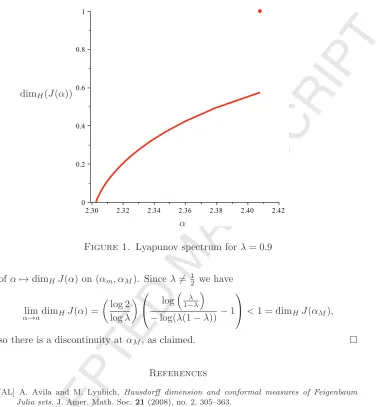
This allows us to deduce the following result, see Figure 1.

Proposition 4.4. Consider the mapFλ forλ∈(12,1). Then for anyt > − log 2 logλ ,

dim_HJ

−log(1−λ)−λ

t_logλ

1−λt

= tlog(1−λ)−log(1−λ

t₎

−log(1−λ)−λ₁t₋log_λtλ

+t. (11)

and dimH(J(−logλ(1−λ))) = 1. In particular the function α → dimHJ(α) is

analytic in(αm, αM)but discontinuous at αM.

Proof. Given t > −_loglog 2_λ , set α_t :=

−log(1−λ)−λ₁t₋log_λtλ

. Then defining g : (−log 2/logλ,∞) → R by g(t) = P(−tφ), we obtain g(t) = −αt. Moreover by

the results in [BT1] it follows that for t in our specified range, the potential −tφ has an unique equilibrium state μt with λ(μt) = αt and _λh((μμtt)) = g(t)/αt+t. If we let μbe anF_λ invariant measure such that λ(μ) = α_t then by the Variational Principle, h(μ) ≤ h(μt). Therefore _λh((μμ)) ≤ g(t)/αt+t and thus dimH(JR(α)) = V(α) =g(t)/α_t+t. We next check the range of values ofαfor which equation (11) holds. Clearly, lim_t−log 2

α dim_H(J(α))

Figure 1. Lyapunov spectrum forλ= 0.9

ofα→dim_HJ(α) on (α_m, α_M). Sinceλ= 1₂ we have

lim

α→adimHJ(α) =

log 2 logλ

⎛ ⎝ log

λ

1−λ

−log(λ(1−λ))−1 ⎞

⎠<1 = dimHJ(αM),

so there is a discontinuity atαM, as claimed.

References

[AL] A. Avila and M. Lyubich, Hausdorff dimension and conformal measures of Feigenbaum Julia sets.J. Amer. Math. Soc.21(2008), no. 2, 305–363.

[Ba] L. Barreira, Dimension and recurrence in hyperbolic dynamics.Progress in Mathematics, 272. Birkhauser Verlag, Basel, 2008.

[BS] L. Barreira and B. Saussol, Variational principles and mixed multifractal spectra. Trans. Amer. Math. Soc.353(2001), no. 10, 3919–3944.

[BSSc] L. Barreira, B. Saussol and J. Schmeling, Higher-dimensional multifractal analysis. J. Math. Pures Appl. (9)81(2002), 67–91.

[BSc] L. Barreira and J. Schmeling,Sets of “non-typical” points have full topological entropy and full Hausdorff dimension. Israel J. Math.116(2000), 29–70.

[BT1] H. Bruin and M. Todd,Transience and thermodynamic formalism for infinitely branched interval maps.J. London Math. Soc.86(2012), 171–194.

[BT2] H. Bruin and M. Todd, Wild attractors and thermodynamic formalism.Monatsh. Math. Monatsh. Math.₁₇₈(2015) 39–83.

[Cl] V. Climenhaga,The thermodynamic approach to multifractal analysis.Ergodic Theory Dy-nam. Systems₃₄(2014), no. 5, 1409–1450.

[C] V. Cyr, Countable Markov shifts with Transient Potentials.Proc. London Math. Soc.₁₀₃ (2011), 923–949.

[Fa] K. Falconer,Fractal geometry. Mathematical foundations and applications.Second edition. John Wiley & Sons, Inc., Hoboken, NJ, 2003.

[FS] K. Falk and B. Stratmann, Remarks on Hausdorff dimensions for transient limit sets of Kleinian groups,Tohoku Math. J. (2)56(2004), no. 4, 571–582.

[FFW] A. Fan, D. Feng and J. Wu,Recurrence, dimension and entropy.J. London Math. Soc. (2)64(2001), no. 1, 229–244.

[FLP] A. Fan, L. Liao and J. Peyri´ere,Generic points in systems of specification and Banach valued Birkhoff ergodic average.Discrete Contin. Dyn. Syst.21(2008), no. 4, 1103–1128. [FLWW] A. Fan, L. Liao, B. Wang and J. Wu.On Khintchine exponents and Lyapunov exponents

of continued fractions,Ergodic Theory Dynam. Systems29(2009), no. 1, 73–109.

[FLW] D. Feng, K-S. Lau and J. Wu,Ergodic limits on the conformal repellers.Adv. Math.169 (2002), no. 1, 58–91.

[GR] K. Gelfert and M. Rams,The Lyapunov spectrum of some parabolic systems,Ergodic Theory Dynam. Systems29(2009), no. 3, 919–940.

[Gu] B.M. Gureviˇc,Topological entropy for denumerable Markov chains,Dokl. Akad. Nauk SSSR

10(1969) 911–915.

[HMU] P. Hanus, R. D. Mauldin and M. Urbanski,Thermodynamic formalism and multifractal analysis of conformal infinite iterated function systems,Acta Math. Hungar.₉₆(2002), no. 1-2, 27–98.

[H] F. Hofbauer,Multifractal spectra of Birkhoff averages for a piecewise monotone interval map. Fund. Math.₂₀₈(2010), no. 2, 95–121.

[HR] F. Hofbauer and P. Raith,The Hausdorff dimension of an ergodic invariant measure for a piecewise monotonic map of the interval.Canad. Math. Bull.35(1992), no. 1, 84–98. [I] G. Iommi,Multifractal analysis for countable Markov shifts.Ergodic Theory Dynam. Systems

25(2005) 1881–1907.

[IJ1] G. Iommi and T. Jordan Multifractal analysis of Birkhoff averages for countable Markov maps.Ergodic Theory Dynam. Systems.35(2015), no. 8, 2559–2586.

[IJ2] G. Iommi and T. JordanMultifractal analysis of quotients of Birkhoff sums for countable Markov maps.Int. Math. Res. Not. IMRN 2, 460–498 (2015).

[IJT] G. Iommi, T. Jordan and M. Todd,Recurrence and transience for suspension flows.Israel J. Math.209(2015), no. 2, 547–592.

[IT] G. Iommi and M. Todd,Transience in Dynamical Systems.Ergodic Theory Dynam. Systems

33(2013), no. 5, 1450–1476.

[JJOP] A. Johansson, T. Jordan, A. Oberg and M. Pollicott, Multifractal analysis of non-uniformly hyperbolic systems.Israel J. Math.₁₇₇(2010), 125–144.

[KMS] M. Kesseb¨ohmer, S. Munday and B. Stratmann,Strong renewal theorems and Lyapunov spectra for a -Farey and a -L¨uroth systems,Ergodic Theory Dynam. Systems₃₂(2012), no. 3, 989–1017.

[KS] M. Kesseb¨ohmer and B. Stratmann,A multifractal analysis for Stern-Brocot intervals, con-tinued fractions and Diophantine growth rates, J. Reine Angew. Math.605(2007), 133–163. [KU] M. Kesseb¨ohmer and M. Urba´nski,Higher-dimensional multifractal value sets for conformal

infinite graph directed Markov systems.Nonlinearity20(2007), no. 8, 1969–1985.

[MS] N. Makarov and S. Smirnov,On “thermodynamics” of rational maps. I. Negative spectrum.

Comm. Math. Phys.211(2000), no. 3, 705–743.

[M] A. Manning, A relation between Lyapunov exponents, Hausdorff dimension and entropy.

Ergodic Theory Dynamical Systems1(1981), no. 4, 451–459.

[MU] R. Mauldin and M. Urba´nski,Graph directed Markov systems: geometry and dynamics of limit sets, Cambridge tracts in mathematics 148, Cambridge University Press, Cambridge 2003.

[N] K. Nakaishi,Multifractal formalism for some parabolic maps,Ergodic Theory Dynam. Sys-tems 20 (2000), no. 3, 843–857.

[O] E. Olivier,Structure multifractale d’une dynamique non expansive d´efinie sur un ensemble de Cantor,C. R. Acad. Sci. Paris S´er. I Math.₃₃₁(2000), no. 8, 605–610.

[Ol] L. Olsen,Multifractal analysis of divergence points of deformed measure theoretical Birkhoff averages., J. Math. Pures Appl. (9)₈₂(2003), no. 12, 1591–1649.

[PW] Y. Pesin and H. Weiss,The multifractal analysis of Birkhoff averages and large deviations.

Global analysis of dynamical systems, 419–431, Inst. Phys., Bristol, 2001.

[PoW] M. Pollicott and H. WeissMultifractal analysis of Lyapunov exponent for continued frac-tion and Manneville-Pomeau transformafrac-tions and applicafrac-tions to Diophantine approxima-tion,Comm. Math. Phys. 207 (1999), no. 1, 145–171.

[PU] F. Przytycki, M. Urba´nski,Conformal Fractals: Ergodic Theory Methods,Cambridge Uni-versity Press 2010.

[Sa1] O. Sarig,Thermodynamic formalism for countable Markov shifts. Ergodic Theory Dynam. Systems19(1999), 1565–1593.

[Sa2] O. Sarig,Phase transitions for countable Markov shifts.Comm. Math. Phys.217(2001), no. 3, 555–577.

[Sa3] O. Sarig,Existence of Gibbs measures for countable Markov shifts, Proc. Amer. Math. Soc.

131(2003), 1751–1758.

[SV] B. Stratmann and R. Vogt, Fractal dimension of dissipative sets.Nonlinearity 10(1997) 565–577.

[SU] B. Stratmann and M. Urba´nski,Pseudo-Markov systems and infinitely generated Schottky groups.Amer. J. Math.₁₂₉(2007), no. 4, 1019–1062.

[TV] F. Takens and E. Verbitskiy, On the variational principle for the topological entropy of certain non-compact sets.Ergodic Theory Dynam. Systems₂₃(2003), no. 1, 317–348.

Facultad de Matem´aticas, Pontificia Universidad Cat´olica de Chile (PUC), Avenida Vicu˜na Mackenna 4860, Santiago, Chile

E-mail address:[email protected]

URL:_{http://www.mat.puc.cl/~giommi/}

The School of Mathematics, The University of Bristol, University Walk, Clifton, Bris-tol, BS8 1TW, UK

E-mail address:[email protected]

URL:_{http://www.maths.bris.ac.uk/~matmj/}

Mathematical Institute, University of St Andrews, North Haugh, St Andrews, KY16 9SS, Scotland

E-mail address:[email protected]