ISSN Online: 1947-3818 ISSN Print: 1949-243X
DOI: 10.4236/epe.2019.118020 Aug. 16, 2019 320 Energy and Power Engineering
Important Issues and Results When
Considering the Stochastic Representation
of Wind Power Plants in a Generation
Optimization Model: An Application to the
Large Brazilian Interconnected Power System
Juliana F. Chade Mummey
1*, Ildo L. Sauer
1, Dorel S. Ramos
2, William W.-G. Yeh
31Institute of Energy and Environment, University of Sao Paulo, Sao Paulo, Brazil 2Escola Politécnica, University of Sao Paulo, Sao Paulo, Brazil
3Department of Civil and Environmental Engineering, University of California, Los Angeles, USA
Abstract
Wind power has an increasing share of the Brazilian energy market and may represent 11.6% of total capacity by 2024. For large hydro-thermal sys-tems having high-storage capacity, a complementarity between hydro and wind production could have important effects. The current optimization models are applied to dispatch power plants to meet the market demand and optimize the generation dispatches considering only hydroelectric and thermal power plants. The remaining sources, including wind power, small-hydroelectric plants and biomass plants, are excluded from the optimi-zation model and are included deterministically. This work introduces a gen-eral methodology to represent the stochastic behavior of wind production aimed at the planning and operation of large interconnected power systems. In fact, considering the generation of the wind power source stochastically could show the complementarity between the hydro and wind power produc-tion, reducing the energy price in the spot market with the reduction of thermal power dispatches. In addition to that, with a reduction in wind power and a simultaneous dry-season occurrence, this model, is able to show the need of thermal power plants dispatches as well as the reduction of the risk of energy shortages.
Keywords
Stochastic Optimization, Hydrothermal Systems Planning, Wind Power, Complementarity, Synthetic Series Generation
How to cite this paper: Mummey, J.F.C., Sauer, I.L., Ramos, D.S. and Yeh, W.W.-G. (2019) Important Issues and Results When Considering the Stochastic Representation of Wind Power Plants in a Generation Optimization Model: An Application to the Large Brazilian Interconnected Power System. Energy and Power Engineering, 11, 320-332. https://doi.org/10.4236/epe.2019.118020
Received: July 13, 2019 Accepted: August 13, 2019 Published: August 16, 2019
Copyright © 2019 by author(s) and Scientific Research Publishing Inc. This work is licensed under the Creative Commons Attribution International License (CC BY 4.0).
http://creativecommons.org/licenses/by/4.0/
DOI: 10.4236/epe.2019.118020 321 Energy and Power Engineering
1. Introduction
The energy generation in Brazil is dominated by hydropower plants with large reservoirs which are arranged in cascades. It is forecasted to represent 11.6% of the Brazilian installed capacity by 2024 [1]. According to [2], the increase of wind power capacity worldwide in 2017 was 535 GW, reaching a total of 539 GW. China alone installed 19.7 GW in 2017, reaching 188 GW in total. Brazil was sixth in percentage increase in 2017 and is in the top ten countries in terms of total installed capacity.
In September 2016, the capacity factor registered by the state of Rio Grande do Norte was almost 57% and all states of the Northeast had capacity factor higher than 50% [3]. Wind power in the Northeast was able to meet 39% of the demand in this same month, when the reservoir levels were experiencing a shortage (Figure 1).
The Brazilian System Operator (ONS) dispatches the power plants to meet the demand. Cepel, the Brazilian Electric Energy Research Center, implemented the computational program Newave with the stochastic dual dynamic programming (SDDP) technique [4] to solve the large-scale long-term hydrothermal problems for the Brazilian system. The model aims to determine the optimal amount of hydro and thermal resources for operation planning and minimize the expected value of the operation cost [5]. In this study, we use the Newave model for the simulations.
The inflows are represented stochastically in the models as the future is un-known. Uncertainty is represented by a tree of scenarios where each branch of the tree is a hydrologic scenario. The Newave considers the variables’ uncertain-ty through synthetic inflow scenarios to all subsystems [6]. GEVAZP, the syn-thetic inflow scenarios generation model, is connected to the Newave. It selects a stochastic time series PAR (p) algorithm to guarantee similarity between histor-ical and synthetic series [7]. The PAR (p) is an auto regressive periodic function where p can vary from 1 - 6 (months), so each stochastic inflow can be depen-dent on the inflow that occurred in the same places up to 6 months before [8].
[9] shows wind and hydrologic generation scenarios with the same stochastic model PAR (p) for the operation planning and recommends the use of the wind series for the Brazilian planning hydrothermal operation. [10] developed a new methodology to build the scenario trees, removing non-linearity from the equa-tions, which could make the future cost calculation in Newave an unfeasible task. Even though some studies recommend the stochastic model PAR (p), there are some limitations and questions remain whether this model is ideal for wind power series generation.
DOI: 10.4236/epe.2019.118020 322 Energy and Power Engineering
Figure 1. Reservoirs and wind power generation (Source: ONS, 2016-Juliana
Mummey et al.).
[12] analyses the impact of considering the uncertainty of wind power genera-tion scenarios using the model SDDP. The results show an increase of the costs and point out that by changing the future cost methodology the impact could be reduced.
Given the wind power generation variability and considering the increase in the share of wind power in the Brazilian electricity matrix, this paper aims to present a study about the stochastic representation of wind power generation in the Brazilian official models. The impacts on the other source’s generation and when wind power plants are represented as run-of-river power plants, will be discussed ahead.
The current study differs from the existing literature because it uses an opti-mization simulation model (Newave) to represent the wind and hydro genera-tion stochasticity, while previous work doesn’t represent explicitly the wind and hydro production variability. In fact, the correlation between the power genera-tion of these two sources is obtained from the historical registered behavior of the water flows at the main Brazilian river basins and series of wind speed, which were reconstructed based on data obtained from meso-scale meteorological models [13]. In addition to that, this study shows the production complementar-ity between wind and hydro generation as a result of the simulation model when using the stochastic formulation for both kind of sources. It is worthwhile to point out that currently the Brazilian System Operator model considers the wind power deterministically and therefore it does not represent the variability of the wind power source.
This introduction describes the problem focused in this work, a brief survey of the state of the art of wind power in Brazil, expansion perspectives and studies about wind power series. Section 2 shows the methodology involved such as: 1) wind speed database and wind power generation, and 2) wind power representa-tion in the Brazilian system. Secrepresenta-tion 3 shows the results of the simularepresenta-tions: 1) the rebuilt historic of wind power generation (considering the occurrence of
hy-0 500 1,000 1,500 2,000 2,500 3,000 3,500 4,000 4,500 0% 10% 20% 30% 40% 50% 60% 70% 80% 90% Ja n/ 2012 Ap r/ 2012 Ju l/ 2012 O ct /2012 Ja n/ 2013 Ap r/ 2013 Ju l/ 2013 O ct /2013 Ja n/ 2014 Ap r/ 2014 Ju l/ 2014 O ct /2014 Ja n/ 2015 Ap r/ 2015 Ju l/ 2015 O ct /2015 Ja n/ 2016 Ap r/ 2016 Ju l/ 2016 O ct /2016 W in d Po w er G en er at io n ( M W a ve ra ge ) % R es er vo ir St or ag e Le vel s
Reservoir Storage Levels and Wind Power Generation
DOI: 10.4236/epe.2019.118020 323 Energy and Power Engineering
draulic and wind power production varying simultaneously) and comparison to the official historical simulation (average monthly historical values, each month is the same every year); 2) based on “1” and a hypothetic scenario of an increase of wind power capacity and an increase of the Northeast and South demands; and 3) same as “1” but considering synthetic series. Section 4 concludes this ar-ticle.
2. Methodology
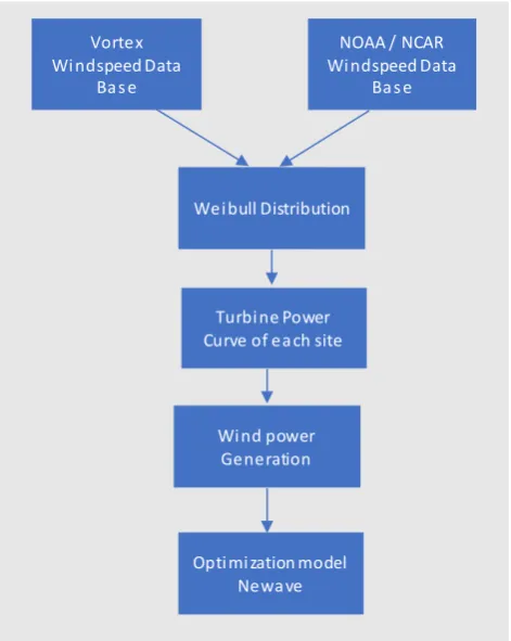
This work uses two sources of wind speed data representing 16 sites in the Northeast and the South of Brazil. We plotted the Weibull distribution to fit the wind speed distribution. Then, a power curve of each site is used to calculate the wind power generation. All this data represents an input to the optimization model Newave in order to run the program. Figure 2 represents the schematic diagram of the methodology.
2.1. Wind Speed and Wind Power Generation
[image:4.595.256.492.407.703.2]The methodology of wind speed historical data reconstruction and its power generation was based on [13]. Two databases were considered: Vortex (Mesos-cale atmospheric model on-line that estimates wind speed for places without measurements) and NOAA (numerical model from National Oceanic and At-mospheric Administration).
Figure 2. Schematic diagram of the methodology.
Vortex Windspeed Data
Base
NOAA / NCAR Windspeed Data
Base
Weibull Distribution
Turbine Power Curve of each site
Wind power Generation
DOI: 10.4236/epe.2019.118020 324 Energy and Power Engineering
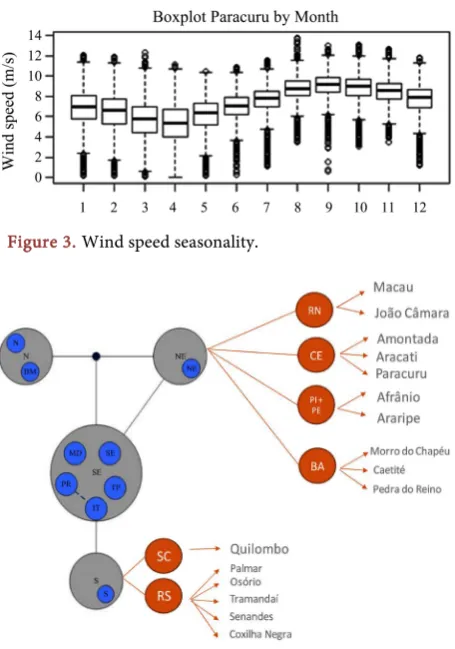
The Vortex database provides the hourly wind speed from 1982 to 2014 for every 10 meters of height, starting at 50 meters up to 150 meters. The NOAA database presents daily values of wind speed at 42 meters since 1947. There were 16 sites considered and Figure 3 shows the seasonality of hourly wind speed data of the site at Paracuru, as an example. It can be observed that there is a trend of higher wind speeds and shorter variability in the second six months of the year.
We transformed both series (NOAA and Vortex) into the same period to be comparable, using the same years from 1982 to 2010 and daily wind speeds. We also considered all series with cross-correlation greater than 0.8 and then a ver-tical extrapolation to transform the NOAA data from 10 meters to 120 meters high with the logarithmic curve with the Vortex data available. We calculated monthly standard deviation with the Vortex data and based on the daily average wind speed we plotted the Weibull distribution (the Weibull probability density function was used to fit the wind speed distribution) for each month. Then we calculated the energy generated with the power curve of each site and the Wei-bull distribution fit to the historical data. Based on the daily wind power genera-tion, we added all days of the month to transform into monthly wind power generation from 1948 to 2014.
2.2. Wind Power Representation
The model Newave has four main subsystems and nine regions: Paraná, Itaipu, Madeira, Teles Pires and Southeast (five regions in the Southeast subsystem); North and Belo Monte (two regions in the North subsystem); Northeast subsys-tem (one region) and South subsyssubsys-tem (one region). The maximum capacity of regions for the model is 15, so we included four regions in the Northeast: CE (Ceará), BA (Bahia), PI + PE (Piauí + Pernambuco) and RN (Rio Grande do Norte), and two regions in the South region: SC (Santa Catarina) and RS (Rio Grande do Sul), as Figure 4. These new regions are wind basins and represent areas of the system with high concentration of sites and a correlated wind re-gime.
Each region has the wind power installed capacity of the state and the respec-tive expansion according to the Monitoring Department of Electric System (DMSE). Each wind power site was included in the program as if it was a run-of-river power plant. As there are many sites, with different seasonalities in-side the same state, we put the values of the closest sites and their expansion ac-cording to where they are in the Abeeólica (Wind Power Association) data [14].
3. Results
DOI: 10.4236/epe.2019.118020 325 Energy and Power Engineering
Figure 3. Wind speed seasonality.
Figure 4. Representation of regions.
cases, we analyze the complementarity of wind power generation with hydro-power, verifying in dry seasons a) if the wind power can generate more; b) if with more wind power capacity, what is the role of wind power generation to meet the demand; and c) if the behavior with synthetic series is compatible with the observed one when using historical series.
We chose two historical critical (dry years) periods to analyze the data. The first one refers to the years 1951 to 1955 (the horizon of Newave is 5 years). These years presented low inflow in the Northeast and re-constructed wind power generation with some months below the average. The second period refers to 2010 to 2014. These years presented low inflow in the Northeast and re-constructed wind power generation above average. Considering the synthetic series, the data are analyzed through the average values.
3.1. Simulation Considering the Wind Power in Regions
DOI: 10.4236/epe.2019.118020 326 Energy and Power Engineering
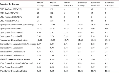
Table 1. Marginal costs and generation.
August of the 4th year Official Average Official 1951-1955 Official 2010-2014 Simulation Average Simulation 1951-1955 Simulation 2010-2014
CMO Southeast (R$/MWh) 28 152 6 9 47 2
CMO South (R$/MWh) 27 152 6 8 47 2
CMO Northeast (R$/MWh) 21 85 6 1 0 0
CMO North (R$/MWh) 24 114 6 7 44 1
Hydropower Generation SE (GW average) 25.96 23.09 27.89 25.80 28.76 21.86
Hydropower Generation S 11.71 11.37 13.74 10.30 6.66 13.63
Hydropower Generation NE 4.88 5.67 3.79 4.48 4.41 4.37
Hydropower Generation N 5.89 5.73 3.29 6.67 7.10 7.10
Hydropower Generation System 48.44 45.86 48.71 47.25 46.93 46.96
Thermal Power Generation SE (GW average) 2.87 3.83 2.71 2.73 2.88 2.71
Thermal Power Generation S 0.81 0.98 0.78 0.78 0.78 0.78
Thermal Power Generation NE 0.58 0.71 0.57 0.57 0.57 0.57
Thermal Power Generation N 1.26 2.59 1.21 1.21 1.21 1.21
Thermal Power Generation System 5.52 8.11 5.27 5.29 5.44 5.27
Wind Power Generation S (GW average) 0.87 0.87 0.87 1.05 1.05 1.15
Wind Power Generation NE 8.26 8.26 8.26 9.49 9.67 9.71
Wind Power Generation System 9.13 9.13 9.13 10.54 10.72 10.86
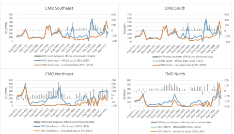
the simulation are lower than in the official case. This happens because, as in the official case, the wind power generation is deterministic and, hence, there is no change of this generation if it is a dry season or not. Considering the simulation, in February of 1955, for example, even though there is a low hydraulic inflow in the Northeast and the re-constructed wind power is also low, there is a higher wind power generation, with less need of thermal power generation, reducing the marginal costs of operation, seeFigure 5. It shows the complementarity of the hydro with the wind power in the Northeast in the simulation. Considering the period of 2010 to 2014, as the re-constructed wind power was higher than in 1951 to 1955, wind power generation could complement even more with the hy-dropower generation, seeTable 1.
DOI: 10.4236/epe.2019.118020 327 Energy and Power Engineering
Figure 5. Marginal costs of the simulation vs. official case.
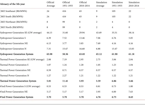
Table 2. Marginal costs and generation.
February of the 5th year Official Average Official 1951-1955 Official 2010-2014 Simulation Average Simulation 1951-1955 Simulation 2010-2014
CMO Southeast (R$/MWh) 24 416 65 9 105 22
CMO South (R$/MWh) 24 416 65 9 105 22
CMO Northeast (R$/MWh) 8 99 0 2 4 0
CMO North (R$/MWh) 8 99 0 2 4 0
Hydropower Generation SE (GW average) 44.13 31.60 29.94 43.49 35.51 38.14
Hydropower Generation S 6.39 7.52 13.46 7.06 6.76 5.05
Hydropower Generation NE 6.15 3.77 3.85 7.69 4.16 4.16
Hydropower Generation N 7.31 15.47 16.60 6.88 15.47 13.83
Hydropower Generation System 63.98 58.36 63.85 65.12 61.90 61.18
Thermal Power Generation SE (GW average) 2.88 7.19 2.95 2.75 3.84 2.84
Thermal Power Generation S 1.07 1.24 1.20 1.05 1.23 1.04
Thermal Power Generation NE 0.59 0.71 0.57 0.57 0.57 0.57
Thermal Power Generation N 1.27 2.27 1.21 1.22 1.22 1.21
Thermal Power Generation System 5.81 11.41 5.93 5.59 6.86 5.66
Wind Power Generation S (GW average) 0.53 0.53 0.53 0.81 0.73 1.00
Wind Power Generation NE 5.17 5.17 5.17 3.95 6.00 7.63
Wind Power Generation System 5.70 5.70 5.70 4.76 6.73 8.63
-400 -200 0 200 400 600
0 100 200 300 400 500 600 700
R$
/MW
h
CMO Southeast
Difference between official and simulated data CMO Southeast - official data (1951-1955) CMO Southeast - simulated data (1951-1955)
-400 -200 0 200 400 600
0 100 200 300 400 500 600 700
R$
/MW
h
CMO South
Difference between official and simulated data CMO South - official data (1951-1955) CMO South - simulated data (1951-1955)
-100 -50 0 50 100 150 200 250
0 50 100 150 200 250 300 350
R$
/MW
h
CMO Northeast
Difference between official and simulated data CMO Northeast - official data (1951-1955) CMO Northeast - simulated data (1951-1955)
-300 -200 -100 0 100 200
0 100 200 300 400 500 600
R$
/MW
h
CMO North
[image:8.595.59.537.394.740.2]DOI: 10.4236/epe.2019.118020 328 Energy and Power Engineering
3.2. Simulation Considering Wind Power in Regions and an
Increase of the Wind Power Capacity
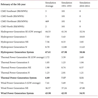
[image:9.595.207.540.395.728.2]This hypothetical case adds 10 times the wind power capacity to the system proportionally to both the Northeast and South subsystems. We used this in-crease as the wind power capacity today represents a tenth of the hydroelectric plants in Brazil and we wanted to understand the impact that the same propor-tion of both sources would represent. It also increases the demand of both sub-systems, otherwise the model would be optimistic. Considering the second six months of the years, the wind power generation can be the main source to at-tend the demand because in this part of the year there are higher wind speeds and greater wind power generation. However, considering the first six months, wind power generation could not be enough to meet the demand and there could be a need to increase hydro and thermal power generation, increasing the marginal cost of the Northeast, once it becomes the region with the most in-crease of the demand. In the example of February, in Table 3, even though it is February and the wind speeds are not high, considering the dry season of 1951-1955, the wind power generation was greater than the average. Considering the years of 2010-2014, the wind power generation is much greater, showing the complementarity of the case.
Table 3. Marginal costs and generation.
February of the 5th year Simulation Average Simulation 1951-1955 Simulation 2010-2014
CMO Southeast (R$/MWh) 3 101 0
CMO South (R$/MWh) 3 101 0
CMO Northeast (R$/MWh) 469 101 0
CMO North (R$/MWh) 2 101 0
Hydropower Generation SE (GW average) 44.33 41.34 32.54
Hydropower Generation S 7.03 5.43 10.03
Hydropower Generation NE 7.56 8.33 3.85
Hydropower Generation N 8.70 12.88 11.63
Hydropower Generation System 67.61 67.98 58.06 Thermal Power Generation SE (GW average) 2.72 3.59 2.69
Thermal Power Generation S 1.05 1.23 1.04
Thermal Power Generation NE 1.90 0.74 0.57
Thermal Power Generation N 1.23 2.01 1.21
Thermal Power Generation System 6.89 7.57 5.51 Wind Power Generation S (GW average) 7.41 5.69 7.91
Wind Power Generation NE 36.57 37.24 47.00
DOI: 10.4236/epe.2019.118020 329 Energy and Power Engineering
3.3. Simulation Considering Wind Power in Regions and Synthetic
Series
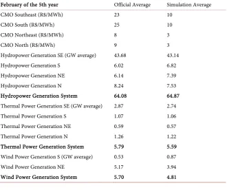
In the case of synthetic series, the marginal costs of the simulation also present reductions in almost all months for all subsystems compared to the official case, seeFigure 6. However, considering February of the last year, which in this case is February of 2020, wind power generation was lower than in the official case with synthetic series in the Northeast and higher in the South, see Table 4.
Even with the lower wind power generation in this specific month, the mar-ginal cost was lower than the official case with synthetic series. This is because as there is more wind power generation in the previous months, the reservoir sto-rage levels are higher and consequently there is more availability of hydropower to generate energy and reduce the costs.
Figure 7 shows that there is more wind power generation in almost all months in the simulation compared to the official case in the Northeast and in the South. However, in the wet season (period between December and April) of the years, wind power in the Northeast showed lower values, emphasizing the seasonality. There is a decrease of marginal costs in the simulation because of the higher hydropower generation. This happens because the storage level of the re-servoirs is higher than the official case, with the higher wind power in previous months.
[image:10.595.209.540.459.735.2]Figure 8 shows the complementarity of the wind power generation with the hydropower generation in the Northeast comparing the official case and the si-mulations and considering synthetic series. As the official case is deterministic, wind power generation considers the same seasonality during those years.
Table 4. Marginal costs and generation.
February of the 5th year Official Average Simulation Average
CMO Southeast (R$/MWh) 23 10
CMO South (R$/MWh) 25 10
CMO Northeast (R$/MWh) 8 3
CMO North (R$/MWh) 9 3
Hydropower Generation SE (GW average) 43.68 43.14
Hydropower Generation S 6.02 6.82
Hydropower Generation NE 6.14 7.39
Hydropower Generation N 8.24 7.53
Hydropower Generation System 64.08 64.87
Thermal Power Generation SE (GW average) 2.87 2.74
Thermal Power Generation S 1.07 1.06
Thermal Power Generation NE 0.59 0.57
Thermal Power Generation N 1.26 1.22
Thermal Power Generation System 5.79 5.59
Wind Power Generation S (GW average) 0.53 0.87
Wind Power Generation NE 5.17 3.94
DOI: 10.4236/epe.2019.118020 330 Energy and Power Engineering
[image:11.595.57.540.376.523.2]Figure 6. Marginal costs of the simulation vs. Official case with synthetic series.
Figure 7. Wind power generation vs. official case with synthetic series.
Figure 8. Complementarity of hydropower and wind power generation.
-400 -200 0 200 400 600 0 100 200 300 400 500 600 700 R$ /MW h CMO Southeast
Difference between official and simulated data CMO Southeast - official data (1951-1955) CMO Southeast - simulated data (1951-1955)
-400 -200 0 200 400 600 0 100 200 300 400 500 600 700 R$ /MW h CMO South
Difference between official and simulated data CMO South - official data (1951-1955) CMO South - simulated data (1951-1955)
-100 -50 0 50 100 150 200 250 0 50 100 150 200 250 300 350 R$ /MW h CMO Northeast
Difference between official and simulated data CMO Northeast - official data (1951-1955) CMO Northeast - simulated data (1951-1955)
-300 -200 -100 0 100 200 0 100 200 300 400 500 600 R$ /MW h CMO North
Difference between official and simulated data CMO North - official data (1951-1955) CMO North - simulated data (1951-1955)
-3000 -2000 -1000 0 1000 2000 3000 0 2000 4000 6000 8000 10000 12000 Au g/ 2016 N ov /2016 Fe b/ 2017 M ay /2017 Au g/ 2017 N ov /2017 Fe b/ 2018 M ay /2018 Au g/ 2018 N ov /2018 Fe b/ 2019 M ay /2019 Au g/ 2019 N ov /2019 Fe b/ 2020 M ay /2020 Au g/ 2020 N ov /2020 MW m
Wind power in the Northeast
Difference between official and simulated data Wind power in the Northeast - official data Wind power in the Northeast - simulated data
-500 -400 -300 -200 -100 0 0 200 400 600 800 1000 1200 Au g/ 2016 N ov /2016 Fe b/ 2017 M ay /2017 Au g/ 2017 N ov /2017 Fe b/ 2018 M ay /2018 Au g/ 2018 N ov /2018 Fe b/ 2019 M ay /2019 Au g/ 2019 N ov /2019 Fe b/ 2020 M ay /2020 Au g/ 2020 N ov /2020 MW m
Wind power in the South
Difference between official and simulated data Wind power in the South - official data Wind power in the South - simulated data
0 2,000 4,000 6,000 8,000 10,000 12,000 Au g/ 20 16 Oc t/2 01 6 De c/ 20 16 Fe b/ 20 17 Ap r/ 201 7 Ju n/ 20 17 Au g/ 20 17 Oc t/2 01 7 De c/ 20 17 Fe b/ 20 18 Ap r/ 201 8 Ju n/ 20 18 Au g/ 20 18 Oc t/2 01 8 De c/ 20 18 Fe b/ 20 19 Ap r/ 201 9 Ju n/ 20 19 Au g/ 20 19 Oc t/2 01 9 De c/ 20 19 Fe b/ 20 20 Ap r/ 202 0 Ju n/ 20 20 Au g/ 20 20 Oc t/2 02 0 De c/ 20 20 MW m
Wind power and Hydro power in the Northeast (Simulated data)
Wind power generation in the Northeast Hydro power generation in the Northeast
0 1,000 2,000 3,000 4,000 5,000 6,000 7,000 8,000 9,000 Au g/ 20 16 Oc t/2 01 6 De c/ 20 16 Fe b/ 20 17 Ap r/ 201 7 Ju n/ 20 17 Au g/ 20 17 Oc t/2 01 7 De c/ 20 17 Fe b/ 20 18 Ap r/ 201 8 Ju n/ 20 18 Au g/ 20 18 Oc t/2 01 8 De c/ 20 18 Fe b/ 20 19 Ap r/ 201 9 Ju n/ 20 19 Au g/ 20 19 Oc t/2 01 9 De c/ 20 19 Fe b/ 20 20 Ap r/ 202 0 Ju n/ 20 20 Au g/ 20 20 Oc t/2 02 0 De c/ 20 20 MW m
Wind power and Hydro power in the Northeast (Official data)
[image:11.595.57.546.559.701.2]DOI: 10.4236/epe.2019.118020 331 Energy and Power Engineering
4. Final Remarks and Conclusions
The aim of this work was to present a study to stochastically represent wind power generation in the optimization model (Newave) of the Brazilian electricity system, also, to evaluate how the complementarity of wind power with hydro-power can influence the hydro and thermal hydro-power dispatches considering varia-bility of the wind power source, as well as the consequences for the short-term marginal prices and spot market prices.
There were three simulations comparing the official case with the wind power represented in regions with historical and synthetic series. The results presented were similar from the conceptual and qualitative point of view. In most of these cases, there is a reduction in the marginal costs of operation with the simulation and less variability in the costs. It happened because there is more complemen-tarity in these cases, reducing the need of thermal dispatch to meet the demand. In a deterministic simulation, as nowadays state of the art, the huge variability of the wind power production is not considered and, as a consequence, the com-plementarity effect between hydro and wind generation is not taken into account as an important benefit to the System.
When wind power capacity was increased, it was used as the main source to meet the demand. In the second six months, there were no problems for supplying the demand, because the wind power generation is high in these periods. However, considering the first six months, the simulation showed that the wind power was not enough to attend the demand, lessening the system reliability. These scenarios of different seasons are not represented in the deterministic models, which show the relevance of considering such scenarios.
Considering synthetic series there is also an increase of wind power genera-tion in most of the scenarios, reducing the marginal costs of operagenera-tion. However, we observe that in some wet periods of the years, wind power generation was lower than the official case, showing the complementarity and seasonality of the source, highlighted even more with the stochastic representation of wind power.
This is a case study specific for the Brazilian system but presents methodology that can be replicated to problems of the same nature in any part of the world. To conduct a more detailed analysis we recommend 1) the use of a database with wind speed measurements with anemometers together with a re-analysis data-base; and 2) the use of a higher number of sites, covering greater parts of the re-gions.
Finally, it is important to emphasize that this work does not intend to forecast wind power generation, but rather to show that the deterministic methodology considered in the optimization models of the Brazilian system needs to be ree-valuated.
Conflicts of Interest
DOI: 10.4236/epe.2019.118020 332 Energy and Power Engineering
References
[1] EPE (2016) Decade Energy Plan 2024. EPE, Rio de Janeiro. http://www.epe.gov.br [2] GWEC (2017) Global Wind Report—Annual Market.
http://files.gwec.net/files/GWR2017.pdf
[3] ONS (2016) National Operator of the System. Wind Power Monthly Report Sep-tember/2016. http://www.ons.org.br
[4] Pereira, M.V.F. and Pinto, L.M.V.G. (1991) Multi-Stage Stochastic Optimization Applied to Energy Planning. Mathematical Programming, 52, 359-375.
https://doi.org/10.1007/BF01582895
[5] Maceira, M.E.P., Duarte, V.S., Penna, D.D.J., Moraes, L.A.M. and Melo, A.C.G. (2008) Ten Years of Application of Stochastic Dual Dynamic Programming in Offi-cial and Agent Studies in Brazil—Description of the NEWAVE Program. 16th Power Systems Computation Conference, Glasgow, July 2008.
[6] Maceira, M.E.P. and Mercio, C.M.V.B. (1997) Stochastic Streamflow Model for Hy-droelectric Systems. 5th International Conference PMAPS—Probabilistic Methods Applied to Power Systems, Vancouver, September 1997.
[7] Castro, C.M.B., Marcato, A.L.M., Souza, R.C., Silva Junior, I.C., Oliveira, F.L.C. and Pulinho, T. (2015) The Generation of Synthetic Inflows via Bootstrap to Increase the Energy Efficiency of Long-Term Hydrothermal Dispatches. Electric Power Sys-tems Research, 124, 33-46.https://doi.org/10.1016/j.epsr.2015.02.014
[8] CCEE, ONS (2015) The Interconnected System and the Models for Energy Opera-tion Planning.
[9] Machado, R.C. (2016) Hydro and Wind Scenarios Generation for Planning of Energy Operation with Autoregressive Model. Master Thesis, University of Santa Catarina, Florianópolis.
[10] Oliveira, F.L.C. (2013) Time Series Model for Stochastic Optimizations. Doctorate Thesis, Electrical Engineering Post Graduation. PUC-Rio.
[11] Cesar, T.C., David, P.A.M.-S., Pereira, A.O., Souza, R.A. and Carvalho, R.N.F. (2011) Regularization of Energy Supply—The Role of Complementarity. Electrical Systems Planning Study Group XXI SNPTEE.
[12] El-Heri, Y.S., Borba, B.S., Bezerra, B., Carvalho, M.R.M. and Dall’orto, C.E.R.C. (2016) Analysis of the Energy Impact of the Variability of Wind Energy Production in the Brazilian Electric System. Brazil Wind Power.
[13] Witzler, L.T., Ramos, D.S., Camargo, L.A.S. and Guarnier, E. (2016) Reconstruction of Wind Generation Historical Series Aiming at the Analysis of Energy Comple-mentarity: Methodology and Applications. 13th International Conference on the European Energy Market, Porto, 6-9 June 2016.
https://doi.org/10.1109/EEM.2016.7521324