Munich Personal RePEc Archive
Optimal asymmetric taxation in a
two-sector model with population ageing
Fedotenkov, Igor
Bank of Lithuania, Lithuanian Institute of Agrarian Economics
9 July 2015
Online at
https://mpra.ub.uni-muenchen.de/66053/
Optimal asymmetric
taxation in a two-sector
model with population
ageing
Igor Fedotenkov
1
Bank of Lithuania
Abstract
This paper presents a simple condition for optimal asymmetric labour (capi-tal) taxation/subsidization in a two-sector model with logarithmic utilities and Cobb-Douglas production functions, linked to demographic factors: fertility rate and longevity. The paper shows that depending on parameter values, it may be optimal to tax or subsidize labour in the sectors. If it is optimal to tax the investment-goods sector, a Pareto-improving tax reform is possible. Larger output elasticities of capital in the sectors reduce the possibilities of a Pareto-improving reform, while population ageing in terms of higher longevity enhances the possibilities of welfare improvement for all generations. Fertility rates do not affect optimal taxation.
JEL Classification: E62, H21, J10
Keywords: Two sectors, factor mobility, asymmetric taxation, optimality, population ageing
1
Economics Department, Bank of Lithuania; Lithuanian Institute of Agrarian Economics
1
Introduction
In this paper we develop a rule for optimal sector-specific taxation and subsidiza-tion of producsubsidiza-tion factors in a two-sector, two-overlapping-generasubsidiza-tion model, and link it to demographic factors such as longevity and population growth. The main goal of our paper is to investigate the effects of population ageing on optimal sector-specific production factors taxation. We find that this taxation always leads to welfare improvement in the long run and a condition is de-rived when it is welfare-improving for transitional generations, implying that a Pareto-improving reform is possible. We show that an increase in longevity pos-itively affects the optimal tax rate to be levied on the investment-goods sector, and permits the government to institute welfare-improving taxation. Further-more, the larger the output elasticities of capital, the smaller the optimal tax on labour income in the investment-goods sector. Changes in fertility rates do not affect optimal taxation in the long run.
In one-sector models, the golden rule has been known since the seminal work of Phelps (1961). This was extended by Cremers (2006) to a two-overlapping-generation model with two sectors. In this case, the condition is similar to the standard golden rule in a one-sector model. If capital is overaccumulated rela-tive to the golden rule, the model exhibits dynamic inefficiency, leading to the possibility of a welfare improving reform. If the economy is dynamically efficient - agents’ savings and, hence, capital accumulation are not optimal either, but a Pareto-improving reform is not possible, since it causes losses at least for one transitional generation.
Economies are usually not in their golden rules, because individuals, which make savings-consumption decisions, consider macroeconomic factors as given. They do not take into account that their savings may have an effect on the total capital amount in the economy. But, in the general equilibrium, agents’ savings determine capital-labour ratios, and, therefore, produce externalities on other agents. As a result, agents’ savings/consumption decisions are, in general, far from optimal. In a two-sector model, agents also make other decisions: they choose sectors for working and investment. Definitely, they make these decisions thinking over their own incomes only, and not taking into account that their decisions may have general equilibrium effects. As a result, allocation of production factors between sectors may be far from optimal too. Moreover, in the model with two sectors, agents also produce another source of externalities: agents’ decisions in which sector to work affect returns to capital in the sectors and price of consumption goods, producing an externality on the current old generation. This type of externality is not present in the standard one-good models, consequently we derive a different optimality condition.
allocation of production factors between the sectors. The reverse link also holds: if factors’ allocation between the sectors is suboptimal - agents’ savings, and, hence, consumptions are suboptimal too. The goal of this paper is to explore this reverse link. We derive a condition for optimality different from the standard golden rule.
Two-sector models with investment and consumption goods were first in-troduced by Uzawa (Uzawa 1961; Uzawa 1963) who showed that steady state growth exists, and that the system starting at any initial capital and labour values approaches this steady growth. Galor (1992) extended the Uzawa model with overlapping generations, and found sufficient conditions for a globally-unique equilibrium in a very general setting. In a similar model, Venditti (2005) noted a saddle-point equilibrium stability if the steady state is unique.
The relevant literature also includes Selim (2009, 2010, 2011) who analyzed an optimal taxation of labour and capital in three different settings, all with sim-ilar results. Selim found that it is optimal to impose capital-income tax in the investment-goods sector, and diverse labour-income taxes in the consumption-goods sector. The need for differentiated labour taxation in his model arises only in order to undo inefficiencies caused by asymmetric capital taxation. The main difference between Selim’s and our model is that we study optimal tax-ation accounting for general equilibrium effects, whilst Selim finds optimality conditions with respect to taxes, keeping factor prices fixed. The need for dis-similar labour taxation in our model comes directly from the diverse nature of the goods produced in the sectors: consumption goods directly affect agents’ utilities, but they cannot be invested, whereas investment goods cannot be con-sumed, and do not directly affect utility functions. But a larger amount of investment goods increases capital-labour ratios in the next period, increasing production of consumption goods, which in turn affect agents’ utilities. As a result, under some parameter values it is optimal to tax labour in one sector and subsidize it in another, while under other parameter values an optimal policy may require the opposite. We derive a precise condition for optimal taxation.
Muro (2013) studied optimal taxation of returns to labour and capital in a two-sector general equilibrium model and found that the optimal tax rate on capital income is positive; though Muro did not differentiate taxation between sectors. Unlike Muro (2013) we do not consider capital and labour taxation together, but impose sector-specific labour taxes. In appendix we also present results for a sector-specific capital taxation. Rothschild and Scheuer (2013) also examined optimal taxation in a model with a few sectors. They showed that self-selection into occupational sectors requires less progressive taxes if there are several complementary sectors in an economy.
au-tarky, the gains and losses can be redistributed between the counties so that free trade becomes Pareto-welfare improving. Yakita (2012) has also examined a two-sector model with population ageing. He extended Sayan’s 2×2×2 model adding endogenous fertility, and showed that in such a setting, popula-tion ageing in terms of higher life expectancy does not necessarily induce the export of capital intensive goods from the country. Furthermore, like Sayan, he found that a switch from autarky to an open economy may not lead to welfare improvement. This case would depend on whether the country becomes a net exporter or importer of capital-intensive goods, because longer retirement re-duces number of children, and leads to a smaller demand of consumption goods. The key difference between these models and our own is the question we aim to address. Sayan, Naito and Zhao and Yakita studied the macroeconomic ef-fects of asymmetric population ageing on international trade and the efef-fects of a switch from autarky to free international trade. We extend their models with an asymmetric taxation, and study effects of population ageing on it.
This paper is organized as follows: The next section develops the model and discusses its basic properties. In section 3 a condition for optimal taxation is derived. Section 4 presents a numerical example. Finally, section 5 concludes.
2
The model
We employ a discrete-time Samuelson-Diamond overlapping generations model (Samuelson 1958; Diamond 1965) extended by Galor (1992) with two sectors. There are two overlapping generations and two sectors in the model. One sector (C) produces consumption goods, which can be consumed only, and not stored or invested. Another sector (I) produces investment goods, which can be invested, but not consumed (physical capital). Production factors, labour and capital, are perfectly mobile between the sectors. The general structure of the model is visualised in Figure 1.
We will focus on a labour taxation. In appendix, an asymmetric capital tax-ation, and asymmetric value added taxes (VAT) are analysed. Optimal capital taxation is qualitatively the same as labour taxation in terms of effects con-cerned with all the variables. The case of value added taxes is slightly different, because taxation/subsidization of labour in one sector may lead to subsidiza-tion/taxation of capital in another sector. As young agents supply labour and old generations own the capital, asymmetric value added taxes may lead to an intergenerational reallocation of wealth.
2.1
Firms
Figure 1: General structure of the model
consumption goods using a standard Cobb-Douglas technology:
YC(t) =KCα(t)L 1−α
C (t), (1)
YI(t) =KIβ(t)L 1−β
I (t), (2)
whereαandβ are parameters 0< α, β <1. Wages and interest rates are equal to the marginal returns to labour and capital and they are nominated in terms of consumption goods:
wC(t) = (1−α)kCα(t), (3)
wI(t) = (1−β)p(t)kβI(t), (4)
1 +rC(t) =
α p(t−1)k
α−1
C (t), (5)
1 +rI(t) =
βp(t) p(t−1)k
β−1
I (t). (6)
Wherekx(t) =Kx(t)/Lx(t),x∈ {I, C} are capital-labour ratios. Interest rates
are divided by the price of capital goods in periodt−1: p(t−1), because agents choosing to invest, use their wage incomes expressed in terms of consumption goods to buy investment goods.
2.2
Households
Agents maximize a two-period, log-linear utility function:
U(t) = logCy x(t) +
ψ 1 +ρlogC
o
whereCy
x denotes consumption when young, Cxo is consumption in the second
period of life, ρis a discount factor, ψ ∈ [0,1] is the probability of surviving before the second period of life. This parameter corresponds to longevity.
We assume that annuity markets are perfect, i.e. if a person passes away before his second period of life, his savings are equally redistributed amongst the surviving agents of the same generation, making the real returns to savings equal to 1 +Rx(t) = (1 +rx(t))/ψ.
The budget constraints are:
Cy
x(t) =wx(t)(1−τx)−sx(t), (8)
Cxo(t) = (1 +Rx(t))sx(t), x∈ {C, I}, (9)
whereτx, x∈ {C, I} is a sector specific tax on labour income. The tax can be
negative, representing a subsidy. The maximization problem gives the following expression for savings:
sx(t) =
ψwx(t)(1−τx)
1 +ρ+ψ , x∈ {C, I}. (10)
Instead of the presence of annuity markets we may assume that the assets of agents, who die before their second period of life, are confiscated by the government and are thrown out of the model, for example, to finance external debt. In this case, all the qualitative results of the model remain unchanged.
2.3
Equilibrium and Dynamics
The government levies sector-specific taxes on labour incomes: τI and τC.
Agents may freely choose a sector in which to work. Hence, labour market equilibrium is given as an equality of incomes:
wC(t)(1−τC) =wI(t)(1−τI). (11)
Similarly, capital market equilibrium is described as an equality of interest rates rI(t) =rC(t) =r(t). Combining capital and labour market equilibria together
we get an expression linking sector-specific capital-labour ratios:
kC(t) =
α(1−β)(1−τI)
β(1−α)(1−τC)
kI(t). (12)
As sector specific taxesτI andτC affect the allocation of labour, sector-specific
capital-labour ratios also depend on them. This is an essential difference from the model developed by Cremers (2006).
Price of investment goods in terms of consumption goods can be calculated from equations (3)-(4) and (12):
p(t) =
1−α 1−β
1−α
1−τC
1−τI
1−α
α β
α
Suppose that the size of thet-th generation is Λ(t) =LI(t) +LC(t), and it
grows at a constant rate n: Λ(t)/Λ(t−1) = 1 +n. Because of labour market equilibrium, incomes, and therefore savings in both sectors, are equal; thus, we omit a sector-specific index for savings. Savings are invested in the capital market; therefore, total savings are equal to the output of the investment-goods sector: s(t)Λ(t)/p(t) =YI(t), resulting in:
LI(t)
Λ(t) =
ψ(1−β)(1−τI)
1 +ρ+ψ . (14)
This is an investment good market clearing condition.
One interesting observation is that the allocation of labour between the sectors depends on the tax rate in the investment-goods sector, and not on the tax in the consumption-goods sector. Furthermore, output elasticity of capital in the investment goods sector β affects the allocation of labour, and αdoes not. This finding recalls the results of Jensen (2003), who showed in a slightly different framework without overlapping generations, but with more general production and utility functions, that long-run growth of capital-labour ratios (and, hence, income) decisively depends on the technology parameters of the investment-goods sector, while technology parameters of the consumption-goods sector do not play a significant role in economic growth. Equation (14) also implies that labour immediately reallocates between the sectors when taxation of the investment-goods sector is changed.
Capital depreciates in one period;2 therefore, the amount of capital in the
economy is equal to the total savings made in the previous period, which in turn are limited by the output of investment goods in the economy.
KC(t) +KI(t) =YI(t−1). (15)
implying that
kI(t) =
kβI(t−1) 1 +n
1 + α
β(1−α)(1−τC)
1 +ρ+ψ
ψ −(1−β)(1−τI)
−1
.(16)
Equations (14) and (16) determine the dynamics of the model. Dynamic equation (14) resembles the models with an unstable equilibrium - when, after a structural change, the model immediately jumps to a new steady state; it is however, much simpler. The capital-labour ratio dynamics described by (16) are analysed in Figure 2. As the figure implies, there are two equilibrium points. The equilibriumk∗
I = 0 is unstable and irrelevant for policy analysis. The other
equilibrium is described by equation (17). This is an internal stable equilibrium.
k∗β−1
I = (1 +n)
1 + α
β(1−α)(1−τC)
1 +ρ+ψ
ψ −(1−β)(1−τI)
, (17)
2A more general but less intuitive case, allowing for an incomplete capital depreciation, is
Figure 2: kI(t) dynamics
where k∗
I stands for a steady-state value of the capital-labour ratio. Equation
(17) gives an exact equilibrium capital-labour ratio in the investment-goods sector.
2.4
Government
We suppose that the government’s budget is balanced, and taxes collected in one of the sectors are redistributed in the form of subsidies for people working in another sector: LCwCτC =−LIwIτI. Using labour-market equilibrium this
equality can be rewritten as
τC =−
τIψ(1−β)
1 +ρ+βψ. (18)
Thus, a positive tax in one of the sectors leads to a negative tax (positive subsidy) in another sector.
3
Optimality
Government would prefer tax rateτI so that agents would achieve larger utilities
through parameters and τI only. Hence, p in equation (13) and, hence,
con-sumptions in (8-9) can be expressed through the parameters andτI:
Cy =(1−α)
1−α
(1 +n)1−αβ
α(1−β) β
α
(1 +ρ)(1−τI)α
(1 +ρ+ψ)
1 + τIψ(1−β) 1 +ρ+βψ
1−α
×
1 + α
β(1−α)(1 +τIψ(1−β)
1+ρ+βψ)
1 +ρ+ψ
ψ −(1−β)(1−τI)
−1−αβ
, (19)
Co= ((1−α)β)1−α(1 +n)1−1−α−ββ
(α(1−β)(1−τI))α
(1 +ρ+ψ)
1 + τIψ(1−β) 1 +ρ+βψ
1−α
×
1 + α
β(1−α)(1 + τIψ(1−β)
1+ρ+βψ)
1 +ρ+ψ
ψ −(1−β)(1−τI)
1−1−α−ββ
.(20)
Plugging equations (19-20) into (7) we maximize the utilities of agents work-ing in sector I with respect toτI. Maximization ofYC, with respect toτI leads to
simpler computations, but the same result. The same is also valid when capital is taxed instead of labour. However, in the appendix, where VAT are studied, maximizations ofYC and agents’ utilities give different results because VAT
af-fects agents’ income twice: first, labour income, when young, second, capital income, when old. As a result, there is also an intergenerational reallocation of income. As agents are mobile across the sectors, the other sector’s utility function is maximized as well. Observe that due to the logarithmic form of the utility function, population growth n will not affect optimal taxation. Some cumbersome computations are needed,3 but by equalizing the corresponding
derivative to zero, the expression can be significantly simplified, resulting in the optimal tax rate equal to
τ∗
I =
1−α−β−α(1 +ρ)/ψ
1−β . (21)
Depending on parameter values, labour in sector I may need to be taxed or subsidized in order to reach the optimal allocation of the production fac-tors in equilibrium. The larger the output elasticities of capitalα and β, the smaller the optimal tax or the larger the optimal subsidy for sector I. This is because a larger concentration of resources in the investment-goods sector leads to a larger amount of capital in the following period, which increases outputs in both sectors. If capital plays a minor role in production, it is optimal to tax the investment-goods sector, to increase the production of consumption goods. Greater longevityψenhancesτ∗
I. Indeed, it leads to larger savings and increased
demand for investment goods; but greater demand for investment-goods is out-weighed by a larger demand for consumption goods in the second period of
3Optimization was performed with Maple, and the corresponding file is presented in the
life. Young agents are more interested in increasing their own savings, without taking into account the needs of the old generation, thus underproducing con-sumption goods. Therefore, greater longevity leads to larger optimal taxes on the investment-goods sector. Higher discount rate ρreduces optimal taxes or increases subsidies in sectorI, because, with highρ, agents save not sufficiently for an optimal amount of capital in the economy. Fertility ratendoes not affect the optimal taxation.
Another interesting point can be observed in equation (21): Suppose that initially τI = τC = 0. If τI∗ > 0, and the government decides to tax the
investment-goods sector at the rate τ∗
I, and subsidize the consumption-goods
sector; this can be easily implemented: reallocation of the production factors to the consumption-goods sector increases the number of consumption-goods in the economy and, as a result, agents living at the time of reform may consume more, obtaining larger utilities immediately after the reform is implemented. However, if τ∗
I < 0, and the government sets τI = τI∗, reallocation of
mo-bile production factors to the investment-goods sector reduces production of the consumption-goods in the short run, leading to a decline in utilities of the transitional generations. This effect resembles a familiar property of dynamic (in)efficiency discussed in detail by Cremers (2006); however, the condition is different. In the next subsection we will compare these optimality conditions in more detail, and we will return to the welfare effects of transitional generations later.
3.1
Interest rates
Analysing welfare effects, it is important to find out how interest rates change. Economic literature usually assumes that r > 0, since, if agents store, the amount of goods they obtain in the following period is greater than if those goods had been invested. In our model, annuities also matter, as they change real returns to savings. Furthermore, consumption goods cannot be stored for one period, which amounts to approximately 35 years, and investment goods fully depreciate as well. Agents, therefore, must invest a part of their savings in any case, if they wish to consume in the second period of their lives. Indeed, the case of r < 0 does not seem unrealistic, since, investments in stocks are risky, and agents may never know if they win or lose. Investments in bonds are risky as well, since real returns depend on inflation, and, in general, they can be negative. As our model is deterministic with perfect foresight, agents in the model need not distinguish between stocks and bonds; if they receive positive or negative returns to savings depends on the parameter values. Indeed, plugging equation (18) and (21) into (17) and equation (17) into (6) we get:
r∗=αρn+βψn+αn+αψ+αρ+βψ+α−ψ
(1−α)ψ . (22)
τ∗
I =−r∗
1−α 1−β +
n(αρ+βψ+α)
(1−β)ψ . (23) This gives us a more intuitive explanation of optimal taxation. If population growth n is equal to zero, the investment-goods sector should be taxed when the interest rate is negative (hence, an excess of capital in the economy), and subsidised when the net interest rate is positive (lack of capital in the economy). The second term of this equation corrects for population growth. As the interest rate depends on population growth (equations (17) and (6)) and τ∗
I does not
depend, the presence of the second term removes this dependence. As already mentioned, the introduction ofτ∗
I >0 may be Pareto-improving.
From equation (23) it follows immediately thatτ∗
I >0 if
r∗< n(αρ+βψ+α)
ψ(1−α) . (24)
Cremers (2006) showed that the economy is dynamically inefficient when r∗< n(keeping depreciation rate equal to 1). From the literature we know that
in this case a Pareto-improving reform is possible: if young agents are taxed, and the taxes are reallocated to the old generation in the form of pension benefits, this leads to a Pareto improvement. Taxes for the young and pension benefits for the old - reduce savings, which lowers capital-labour ratios, and increases interest rates, thus the golden rule can be achieved (r∗ = n). The condition
(24) differs from the property of dynamic inefficiency. Larger values of output elasticities of capital αand β make condition (24) more likely to be satisfied than the condition for dynamic inefficiency; the opposite holds when they are small. When condition (24) is satisfied, a Pareto-improving reform is possible via asymmetric taxation. It is explained in more detail in the next section.
The are two factors, which cause suboptimal allocations of production fac-tors. First of all, agents’ choices in which sector to work and to invest determine the amounts of goods produced, and, hence, capital-labour ratios in the next period. As a consequence, agents produce externalities for the future genera-tion, and also on the agents form the same generation in the next period, since capital-labour ratios directly affect interest rates. This factor is intuitively sim-ilar to the property of dynamic (in-)efficiency. There is also another source of externality: the old receive returns on capital both from investment and consumption good sectors; as the old are interested in consumption only (not investment), they are interested in a lower price of consumption goods. The allocation of young agents between the sectors determines the supply of the goods, and this have an important effect on the price of goods, interest rates and welfare of the old. This source of externalities is not present in one-good models. Consequently, we derived a different optimality condition.
agents’ (and capital’s) allocation between the sectors, and the other way around: suboptimal allocation of production factors between the sectors affects intertem-poral allocation of consumption. There is a link between these two sources of inefficiencies, but they are not exactly the same. Sometimes it is easier to correct the intertemporal allocation of resources, and sometimes intratemporal allocation can be readjusted.
Technically, the difference between our condition and Cremers’ is that, in our model, τI affects the agents’ present values of life-time incomes not only
via capital-labour ratios but also directly: wI(1−τI). If this were not the
case, the maximisation problem with respect to τI would be ∂U(·, τI)/∂τI =
∂U(k(τI))/∂τI = [∂U(k(τI))/∂k(τI)][∂k(τI)/∂τI] = 0. ∂k(τI)/∂τI can be
can-celed resulting in∂U(kI)/∂kI = 0 - an optimality condition discussed in details
by Cremers’. That τI directly affects the term wI(1−τI) complicates things,
yielding a condition for the possibility of a Pareto improvement different from the property of dynamic inefficiency. It is interesting to note that when pop-ulation growth is equal to zero (and depreciation rate is equal to unity), both conditions coincide.
Agents make saving-consumption decisions not taking into account that their choices may have general equilibrium effects. Namely, demand for investment and consumption goods determines the relative sizes of the sectors, which affect capital-labour ratios and the welfare of the agents in the following period. As a result, the allocation of labour between sectors may be inefficient, though asymmetric labour taxation can be used as an instrument to overcome these inefficiencies.
4
Numerical example
In this section, two numerical examples are presented to illustrate the welfare effects in both cases: whenτ∗
I >0 andτI∗<0. For this reason, we have chosen
parameter values commonly reported in the literature. The annual discount factor is often chosen to be close to 1% (B¨orsch-Supan, Ludwig, and Winter 2006; Adema, Meijdam, and Verbon 2008). In our model, as the period is approximately equal to 35 years, the discount factor corresponds toρ= 0.4166. Population size att= 0 is normalized to unity and population growthnis set to 0.2, this approximately corresponds to 0.5% annual growth of population due to fertility. Longevityψ here means a survival probability before the next period, and it is presumed to be close to 1 (see Adema et al. (2008), for example). We set it at 0.9. Regarding the output elasticities of capital, these are generally estimated at the 0.3 level or slightly higher (Maddison 1987). We suppose that the investment-goods sector is more capital intensive, thus, we setβ= 0.4, and consider two cases for α: α= 0.2, and α= 0.3. We consider these two cases sinceα= 0.2 results in τ∗
I >0, andα= 0.3 inτI∗<0.
Initially τI =τC = 0. In period t= 0 the government unexpectedly
imple-ments a fiscal reform, settingτI =τI∗, andτC =τC∗ as derived in equations (18)
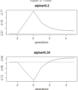
Figure 3 presents the life-time utilities of agents. The horizontal axis corre-sponds to the period when a generation was born. Agents are perfectly mobile between the sectors; therefore, we do not need to distinguish between them. As previously mentioned, in the case ofα= 0.2,τI is positive; therefore, att= 0
agents migrate from sector I to sector C. A decline of labour in the investment-goods sector tends to reduce marginal return to capital in sector I, but increases it in sector C, creating incentives for capital flow to sector C. But, the capital flow is not as large as in one-good models (Geide-Stevenson 1998), because of a price effect: labour outflow raises the cost of investment goods in terms of consumption goods (equation 13), raising the interest rate and reducing capital outflow from sector I. Indeed, capital allocation adjusts as well, but to a lesser degree than in one-good models. The price increase of investment goods leads to higher interest rates after the reform (nominated in consumption goods), and, thus, the consumption of the generation born at t = −1 increases when they are old, leading to a rise in their utilities. The other generations are better off as well.
In the case when α = 0.3, τI < 0; therefore, agents reallocate to the
in-vestment goods sector, leading to a decline in interest rates and losses for the generation born at t = −1. As production of consumption goods declines at t = 0, the generation born at t = 0 is worse off as well. At t = 1, agents enjoy a larger amount of capital in the economy; however, it is not sufficient to make them better off relative to the initial equilibrium. For the given parameter values, only the generations born at t ≥2 are better off. In fact, the benefits accruing to future generations are not sufficient to compensate the losses of the first transitional generations. This property resembles the results of Breyer (1989) and Verbon (1989), who showed that gains of a switch from PAYG to a more-funded pension scheme are not sufficient to reimburse the losses of the transitional generations if the economy is dynamically efficient.
Two panels of figure 3 raise a question what happens between these two values of alpha. It follows from equation (21) that whenα=ψ(1−β)/(1+ψ+ρ), τ∗
I = 0; therefore, labour is allocated efficiently in this case with no need for
government intervention. Figure 4 shows a 3-d dependence of utility on α. It shows that the transition of agents’ utilities depends on whetherαis smaller of greater than this certain value.
Karabarbounis and Neiman (2014) showed that labour shares in production outputs are declining worldwide, raising output elasticities of capital. As per equation (21) and the numerical examples, high output elasticities of capital make implementation of a Pareto-optimal sector-specific taxation impossible. Therefore, policymakers should not delay considering the possibility of such a reform, since, the positive dynamics of size in the output elasticities of capital may continue, thus making a Pareto-efficient reform impossible. Another inter-esting feature is that population ageing in terms of greater longevity (largerψ) enhancesτ∗
I and, hence, augments possibilities for Pareto-improving taxation.
exist in Bulgaria, Germany and Luxemburg. In Ireland, PIT exemptions exist for writers, composers, visual artists and sculptors. But, an asymmetric labour taxation is not usual. However, sector specific VAT is very common. For exam-ple, sector-specific VAT rates are applied in Czech Republic, Estonia, Finland, France and many other countries. We have analysed labour taxation; indeed, the same logic can also be applied for VAT, however, the results are much more complicated, since sector-specific value added taxes not only lead to a intersec-toral reallocation of production factors, but also leads to an intergenerational reallocation, since a tax on labour collected in one sector, may return as a subsidy on capital in another sector (see appendix).
We have noted optimal sector-specific taxation rates assuming specific pro-duction and utility functions. The model can be generalized employing a CES production and/or utility function or an Epstein-Zin utility function (Epstein and Zin 1989) if the number of overlapping generations is enlarged. We expect that such generalizations of the model would also generalize the condition for optimal taxation, which would depend on the generalized functions’ parameters. The model also can be extended with a more realistic overlapping-generation structure, labour market imperfections, bequests, and a large number of other factors.
5
Conclusions
In this paper we derived a condition for optimal sector-specific labour taxation, which maximizes agents’ utilities in the steady state. Depending on specific pa-rameter values, the investment-goods sector should be taxed and consumption-goods sector subsidized, or viceversa. If the optimal tax on the investment consumption-goods sector is positive - an introduction of such a tax is Pareto-improving, based on the assumption that labour and capital are freely mobile between the sectors. If it is optimal to tax the consumption-goods sector, a few transitional generations will be worse off. Larger output elasticities of capital in the sectors reduce the possibilities of a Pareto-improving taxation. Yet, population ageing in terms of greater longevity enhances possibilities of such taxation.
Compliance with Ethical Standards:
Conflict of Interest: The article was written during author’s work in the Bank of Lithuania in 2014. The author has not received any grant, honoraria or financial support apart from his official salary. The author declares that he has no conflict of interest.
References
ageing.Journal of Population Economics 21(4), 933–959.
B¨orsch-Supan, A., A. Ludwig, and J. Winter (2006). Ageing, pension reform, and capital flows: a multicountry simulation model.Economica 73(292), 625–658.
Breyer, F. (1989). On the intergenerational Pareto efficiency of pay-as-you-go financed pension systems. Journal of Institutional and Theoretical Eco-nomics 145, 643–658.
Cremers, E. T. (2006). Dynamic efficiency in the two-sector overlapping gen-erations model.Journal of Economic Dynamics & Control 30(11), 1915– 1936.
Diamond, P. (1965). National debt in a neoclassical growth model.The Amer-ican Economic Review 55(5), 1126–1150.
Epstein, L. G. and S. E. Zin (1989). Substitution, risk aversion, and the tem-poral behavior of consumption and asset returns: A theoretical framework.
Econometrica 57(4), 937–969.
Galor, O. (1992). A two-sector overlapping-generations model: A global char-acterization of the dynamical system.Econometrica 60(6), 1351–1386. Geide-Stevenson, D. (1998). Social security policy and international labor and
capital mobility.Review of International Economics 6(3), 407–416. Jensen, B. S. (2003). Walrasian general equilibrium allocations and dynamics
in two-sector growth models.German Economic Review 4(1), 53–87. Karabarbounis, L. and B. Neiman (2014). The global decline of the labor
share.The Quarterly Journal of Economics 129(1), 61–103.
Maddison, A. (1987). Growth and slowdown in advanced capitalistic economies.Journal of Economic Literature 25, 647–698.
Muro, K. (2013). Optimal labor income taxation in a two-sector dynamic general equilibrium model.International Review of Economics 60(1), 21– 48.
Naito, T. and L. Zhao (2009). Ageing, transitional dynamics, and gains from trade.Journal of Economic Dynamics & Control 33(8), 1531–1542. Phelps, E. (1961). The golden rule of accumulation: A fable for growthmen.
The American Economic Review 51(4), 638–643.
Rothschild, C. and F. Scheuer (2013). Redistributive taxation in the Roy model.The Quarterly Journal of Economics 128(2), 623–668.
Samuelson, P. A. (1958). An exact consumption-loan model of interest with or without the social contrivance of money. Journal of Political Econ-omy 66(6), 467–482.
Sayan, S. (2005). Heckscher-Ohlin revisited: implications of differential pop-ulation dynamics for trade within an overlapping generations framework.
Selim, S. (2009). Optimal capital income taxation in a two sector economy. In: Duffy D, Shinnick E (eds) Public good, public policy and taxation: a European perspective, 4 in new developments in economic research. LIT, Verlag, Berlin.
Selim, S. (2010). Optimal taxation in a two sector economy with heteroge-neous agents.Economics Bulletin 30(1), 534–542.
Selim, S. (2011). Optimal taxation and redistribution in a two sector two class agents’ economy. Cardiff economics working papers, Nr. E2011/6. Uzawa, H. (1961). On a two-sector model of economic growth.The Review of
Economic Studies 29(1), 40–47.
Uzawa, H. (1963). On a two-sector model of economic growth II.The Review of Economic Studies 30(2), 105–118.
Venditi, A. (2005). The two sector overlapping generations model: A simple formulation.Research in Economics 59(2), 164–188.
Verbon, H. A. (1989). Conversion policies for public pensions plans in a small open economy. B. Gustafsson and N. Klevmarken, eds, The Political Econ-omy of Social Security, Elsevier Science, Amsterdam.
Appendix
Capital taxation
In case when capital is taxed instead of labour, real interest rate, which affects consumption when old (equation 9) changes: 1 +Rx(t) = (1 +rx(t))(1−τx)/ψ,
x∈ {I, C}; labour market equilibrium is given by an equality of wages in the sectors: (1−α)kα
C =p(t)(1−β)k β
I; capital market equilibrium is given by an
equality of net capital incomes: αkα−1
C (t)(1−τ˜C) =p(t)βkCβ−1(t)(1−τ˜I), where
˜
τx,x∈ {I, C}denote sector-specific taxes. Dividing labour market equilibrium
by capital market equilibrium we get
kC(t) =
α(1−β)(1−˜τC)
β(1−α)(1−τ˜I)
kI(t). (25)
Equation for savings (10) changes to
sx(t) =
ψwx(t)
1 +ρ+ψ, x∈ {C, I}, (26)
leading to a different expression for share of agents working in the investment-good sector:
LI(t)
Λ(t) =
ψ(1−β)
1 +ρ+ψ. (27)
Equalizing total savings in the economy to the amount of capital, we get an expression for capital-labour ratio in sector I:
k∗β−1
I = (1 +n)
1 + α(1−τ˜I) β(1−α)(1−τ˜I)
1 +ρ+ψ
ψ −1 +β
. (28)
Expression for government budget balance (18) changes as well. Now govern-ment budget is balanced whenKC(1 +rC)˜τC=−KI(1 +rI)˜τI, implying that
˜ τC=−
˜
τIψ(1−α)β
(1 +ρ+βψ)α. (29)
Value added taxes
If VAT taxes are analysed instead of labour taxes, equations (1-11) do not change; however, in equation (9) Rx(t), x ∈ {I, C} changes to 1 +Rx(t) =
(1 +rx(t))(1−τx)/ψ, which does not affect savings.
Capital market equilibrium changes to
αkα−1
C (t)(1−τ˜C) =p(t)βkCβ−1(t)(1−τ˜I). (30)
As a result, equation (12) simplifies to
kC(t) =
α(1−β)
β(1−α)kI(t). (31)
Equations (14-15) do not change, but equation (17) changes to
k∗β−1
I = (1 +n)
1 + α β(1−α)
1 +ρ+ψ
ψ(1−τI)
−(1−β)
, (32)
Government budget constraint changes toYC(t)τC =−pYIτI resulting in
τC=−
ψτI(1−α)
1 +ρ+βψ+ψτI(α−β)
(33)
Having derived capital-labour ratio and government budget constraint, we ex-press all the other variables of interest. We have two opportunities: to maximize agents’ utilities with respect to τI directly, or to maximizeYC. In contrast to
the cases of separate labour and capital taxation, these two methods do not give the same results, because agent’s income is taxed/subsidized twice: first it is taxed/subsidized when young agents receive their wages; next, the income of the old generation is taxed/subsidized. Therefore, a part of the tax for the young, working in one sector, returns as a subsidy for the old, invested to another sec-tor, or vice versa. This produces an intergenerational reallocation of income, and such a reallocation mechanism affects agents’ utilities in a way different from separate labour or capital taxation/subsidization.
Indeed, direct maximization of agents’ utilities has not given us an acceptable analytical solution. But it can be made numerically. For example, for parameter values used in section 4 we received τI = 10.76%, τC = −4.41% for the case
α= 0.2 andτI =−26.64%,τC = 8.63% whenα= 0.3.
The government may choose to maximizeYC. Then, the optimization
prob-lem givesτIexactly as in the case of labour taxation (equation 21), and taxes for
consumption taxes are given by equation (33). For the parameter values used in section 4 this results inτI = 14.20%,τC =−5.84% for the caseα= 0.2 and
τI =−11.06%,τC = 5.97% whenα= 0.3. Intuitively, it is clear, that ifYC is
General depreciation rate
Suppose that capital depreciates incompletely in one period, and denote its depreciation rate asδ. Then equations (5-6) change in the following way:
δ+rC(t) =
α p(t−1)k
α−1
C (t), (34)
δ+rI(t) =
βp(t) p(t−1)k
β−1
I (t). (35)
Furthermore, equation (15) changes to
KC(t) +KI(t) = (1−δ) KC(t−1) +KI(t−1)
+YI(t−1), (36)
leading to a change in the dynamic equation (16):
kI(t−1)β
kI(t)−k(t−1)(1−δ)/(1 +n)
=
(1 +n)
1 + α
β(1−α)(1−τC)
1 +ρ+ψ
ψ −(1−β)(1−τI)
. (37)
A stable equilibrium exists whenδ >−n. This condition is very intuitive: The size of population should not decrease at the rate higher than the rate of capital depreciation. Then, the corresponding capital-labour ratio can be expressed as
k∗β−1
I =
(1 +n)(δ−n) (1−n) ×
1 + α
β(1−α)(1−τC)
1 +ρ+ψ
ψ −(1−β)(1−τI)
. (38)
Government budget constraint and optimization problem give exactly the same optimal tax rates as those described by equations (18) and (21) due to the log-arithmic utility function; however, optimality condition (24) changes. Namely, equation (23) changes to
r∗=−δ(1−β)
(1−α)τ
∗
I +
n
2βψδ+ 2αδ(1 +ρ)−βψ−α(1 +ρ)−βψn−αn(1 +ρ)
ψ(1−α)(1−n)
; (39)
therefore, Pareto-optimal taxation is possible when
r∗< n
2βψδ+ 2αδ(1 +ρ)−βψ−α(1 +ρ)−βψn−αn(1 +ρ)
ψ(1−α)(1−n)
. (40)