Finite sample and asymptotic analysis of generalization ability with an application to penalized regression

Munich Personal RePEc Archive

Finite-sample and asymptotic analysis of

generalization ability with an application

to penalized regression

Xu, Ning and Hong, Jian and Fisher, Timothy

School of Economics, University of Sydney, School of Economics,

University of Sydney, School of Economics, University of Sydney

10 September 2016

Finite-sample and asymptotic analysis of generalization ability with an

application to penalized regression

Ning Xu

School of Economics, University of Sydney

Jian Hong

School of Economics, University of Sydney

Timothy C.G. Fisher

School of Economics, University of Sydney

Abstract

In this paper, we study the performance of extremum estimators from the perspective of

generalization ability (GA): the ability of a model to predict outcomes in new samples from the

same population. By adapting the classical concentration inequalities, we derive upper bounds on the empirical out-of-sample prediction errors as a function of the in-sample errors, in-sample data

size, heaviness in the tails of the error distribution, and model complexity. We show that the error

bounds may be used for tuning key estimation hyper-parameters, such as the number of foldsKin cross-validation. We also show howKaffects the bias-variance trade-off for cross-validation. We demonstrate that theL_{2-norm difference between penalized and the corresponding un-penalized}

regression estimates is directly explained by the GA of the estimates and the GA of empirical moment conditions. Lastly, we prove that all penalized regression estimates areL2-consistent for

both then>pand then<pcases. Simulations are used to demonstrate key results.

Keywords: generalization ability, upper bound of generalization error, penalized regression,

cross-validation, bias-variance trade-off,L_{2difference between penalized and unpenalized regression,}

lasso, high-dimensional data.

✩_{The authors would like to thank Mike Bain, Colin Cameron, Peter Hall and Tsui Shengshang for valuable comments}

on an earlier draft. We would also like to acknowledge participants at the 12th International Symposium on Econometric Theory and Applications and the 26th New Zealand Econometric Study Group as well as seminar participants at Utah, UNSW, and University of Melbourne for useful questions and comments. Fisher would like to acknowledge the financial support of the Australian Research Council, grant DP0663477.

Email addresses:♥✳①✉❅s②❞♥❡②✳❡❞✉✳❛✉(Ning Xu),❥✐❛♥✳❤♦♥❣❅s②❞♥❡②✳❡❞✉✳❛✉(Jian Hong),

Finite-sample and asymptotic analysis of generalization ability with an

application to penalized regression

1. Introduction

Traditionally in econometrics, an estimation method is implemented on sample data in order to infer patterns in a population. Put another way, inference centers on generalizing to the population

the pattern learned from the sample and evaluating how well the sample pattern fits the population.

An alternative perspective is to consider how well a sample pattern fits another sample. In this paper, we study the ability of a model estimated from a given sample to fit new samples from

the same population, referred to as thegeneralization ability(GA) of the model. As a way of

evaluating the external validity of sample estimates, the concept of GA has been implemented in recent empirical research. For example, in the policy evaluation literature (Belloni et al., 2013;

Gechter, 2015; Dolton, 2006; Blundell et al., 2004), the central question is whether any treatment

effect estimated from a pilot program can be generalized to out-of-sample individuals. Similarly, for economic forecasting, Stock and Watson (2012) used GA as a criterion to pick optimal weight

coefficients for model averaging predictors. Generally speaking, a model with higher GA will be

more appealing for policy analysis or prediction.

With a new sample at hand, GA is easily measured using validation or cross-validation to

measure the goodness of fit of an estimated model on out-of-sample data. Without a new sample,

however, it can be difficult to measure GAex ante. In this paper, we demonstrate how to quantify the GA of an in-sample estimate when only a single sample is available by deriving upper bounds

on the empirical out-of-sample errors. The upper bounds on the out-of-sample errors depend on

the sample size, an index of the complexity of the model, a loss function, and the distribution of the underlying population. As it turns out, the bounds serve not only as a measurement of GA, but

also illustrate the trade-off between in-sample fit and out-of-sample fit. By modifying and adapting

the bounds, we are also able to analyze the performance ofK-fold cross-validation and penalized regression. Thus, the GA approach yields insight into the finite-sample and asymptotic properties

of penalized regression as well as cross-validation.

As well as being an out-of-sample performance indicator, GA may also be used for model selection. Arguably, model selection is coming to the forefront in empirical work given the

increasing prevalence of high-dimensional data in economics and finance. We often desire a smaller set of predictors in order to gain insight into the most relevant relationships between outcomes and

covariates. Model selection based on GA not only offers improved interpretability of an estimated

model, but, critically, it also improves the bias-variance trade-off relative to the traditional extremum estimation approach.

1.1. Traditional approach to the bias-variance trade-off

Without explicitly introducing the concept of GA, the classical econometrics approach to model

selection focusses on the bias-variance trade-off, yielding methods such as the information criteria (IC), cross-validation, and penalized regression. For example, an IC may be applied to linear

regression

whereY _∈Rn_{is a vector of outcome variables,X∈}Rn×p_{is a matrix of covariates andu∈}Rn_{is a}

vector of i.i.d. random errors. The parameter vectorβ ∈Rp_{may be sparse in the sense that many}

of its elements are zero. Model selection typically involves using a score or penalty function that

depends on the data (Heckerman et al., 1995), such as the Akaike information criterion (Akaike, 1973), Bayesian information criterion (Schwarz, 1978), cross-validation errors (Stone, 1974, 1977)

or the mutual information score among variables (Friedman et al., 1997, 2000).

An alternative approach to model selection is penalized regression, implemented through the objective function:

min

b_λ

1

n(kY−X bλk2)

2₊

λkb_λkγ (1)

where_{k · k}γ is theLγ norm andλ >0 is a penalty parameter. One way to derive the penalized

regression estimatesbλ is through validation, summarized in Algorithm 1.

Algorithm 1: Penalized regression estimation under validation

1. Setλ=0.

2. Partition the sample into a training setT and a test setS. Standardize all variables (to ensure the penalized regression residualesatisfiesE_{(e) =0 inT andS).}

3. Compute the penalized regression estimateb_λ onT. Useb_λ to calculate the prediction error onS.

4. Increaseλ by a preset step size. Repeat 2 and 3 untilbλ=0.

5. Selectbpento be thebλthat minimizes the prediction error onS.

As shown in Algorithm 1, validation works by solving the constrained minimization problem in

eq. (1) for each value of the penalty parameterλ to derive ab_λ. When the feasible range ofλ is exhausted, the estimate that produces the smallest out-of-sample error among all the estimated

{b_λ}is chosen as the penalized regression estimate,bpen.

Note in eq. (1) that ifλ =0, the usual OLS estimator is obtained. The IC can be viewed as special cases withλ =1 andγ=0. The lasso (Tibshirani, 1996) corresponds to the case with γ=1 (anL_{1penalty). Whenγ=2 (an}L_{2penalty), we have the familiar ridge estimator (Hoerl} and Kennard, 1970). For anyγ >1, we have the bridge estimator (Frank and Friedman, 1993), proposed as a generalization of the ridge.

A range of consistency properties have been established for the IC and penalized regression.

Shao (1997) proves that various IC and cross-validation are consistent in model selection. Breiman (1995); Chickering et al. (2004) show that the IC have drawbacks: they tend to select more variables

than necessary and are sensitive to small changes in the data. Zhang and Huang (2008); Knight

and Fu (2000); Meinshausen and Bühlmann (2006); Zhao and Yu (2006) show thatL_1-penalized regression is consistent in different settings. Huang et al. (2008); Hoerl and Kennard (1970) show

the consistency of penalized regression withγ>1. Zou (2006); Caner (2009); Friedman et al. (2010)

propose variants of penalized regression in different scenarios and Fu (1998) compares different penalized regressions using a simulation study. Alternative approaches to model selection, such as

high-dimensional data.1

1.2. Major results and contribution

A central idea in this paper is that the analysis of GA is closely connected to the bias-variance

trade-off. We show below that, loosely speaking, a model with superior GA typically achieves

a better balance between bias and variance. Put another way, GA can be though of as a way to understand the properties of model selection methods. By the same token, model selection can

be thought of as a tool for GA: if the goal is to improve the GA of a model, model selection is necessary. From the joint perspective of GA and model selection, we unify the class of penalized

regressions withγ>0, and show that the finite-sample and asymptotic properties of penalized

regression are closely related to the concept of GA.

Thefirst contributionof this paper is to derive an upper bound for the prediction error on

out-of-sample data based on the in-sample prediction error of the extremum estimator and to characterize

the trade-off between in-sample fit and out-of-sample fit. As shown in Vapnik and Chervonenkis (1971a,b); McDonald et al. (2011); Smale and Zhou (2009); Hu and Zhou (2009), the classical

concentration inequalities underlying GA analysis focus on the relation between the population

error and the empirical in-sample error. In contrast, we quantify a bound for the prediction error of the extremum estimate from in-sample data on any out-of-sample data. The bound also highlights

that the finite-sample and asymptotic properties of many penalized estimators can be framed in

terms of GA. Classical methods to improve GA involve computing discrete measures of model complexity, such as the VC dimension, Radamacher dimension or Gaussian complexity. Discrete

complexity measures are hard to compute and often need to be estimated. In contrast, we show that

finite-sample GA analysis is easy to implement via validation or cross-validation and possesses desirable finite-sample and asymptotic properties for model selection.

Asecond contributionof the paper is to show that GA analysis may be used to choose the

tuning hyper-parameter for validation (i.e., the ratio of training sample size to test sample size) or cross-validation (i.e., the number of foldsK). Existing research has studied cross-validation for parametric and nonparametric model estimation (Hall and Marron, 1991; Hall et al., 2011; Stone,

1974, 1977). In contrast, by adapting the classical error bound inequalities that follow from GA analysis, we derive the optimal tuning parameters for validation and cross-validation in a model-free

setting. We also show howKaffects the bias-variance trade-off for cross-validation: a higherK

increases the variance and lowers the bias.

Athird contributionof the paper is use GA analysis to derive the finite-sample and asymptotic

properties, in particular that ofL_{2-consistency, for any penalized regression estimate. Various} properties for penalized regression estimators have previously been established, such as probabilistic

consistency or the oracle property (Knight and Fu, 2000; Zhao and Yu, 2006; Candes and Tao,

2007; Meinshausen and Yu, 2009; Bickel et al., 2009). GA analysis reveals that similar properties can be established more generally for a wider class of estimates from penalized regression. We also

1_{Chickering et al. (2004) point out that the best subset selection method is unable to deal with a large number of}

show that theL_{2-difference between the OLS estimate and any penalized regression estimate can} be quantified by their respective GAs.

Lastly, afourth contributionof the paper is that our results provide a platform to extend GA

analysis to time series, panel data and other non-i.i.d. data. The literature has demonstrated that the major tools of GA analysis can be extended to non-i.i.d. data: many researchers have generalized

the VC inequality (Vapnik and Chervonenkis, 1971a,b)—one of the major tools in this paper to

analyze i.i.d. data—to panel data and times series. Other studies show a number of ways to control for heterogeneity, which guarantees the validity of GA analysis. In addition, other tools used in this

paper, such as the Glivenko-Cantelli theorem, the Hoeffding and von Bahr-Esseen bounds, have

been shown to apply to non-i.i.d. data.2Hence, by implementing our framework with the techniques listed above, we can extend the results in this paper to a rich set of data types and scenarios.

The paper is organized as follows. In Section 2 we review the concept of GA, its connection

to validation and cross-validation and derive upper bounds for the finite-sample GA of extremum estimates. In Section 3, we implement the results in the case of penalized regression and show

that properties of penalized regression estimates can be explained and quantified by their GA.

We also prove theL_{2-consistency of penalized regression estimates for both p}6nand p>n

cases. Further, we establish the finite-sample upper bound for theL_{2-difference between penalized}

and unpenalized estimates based on their respective GAs. In Section 4, we use simulations to demonstrate the ability of penalized regression to control for overfitting. Section 5 concludes with

a brief discussion of our results. Proofs are contained in Appendix 1 and graphs of the simulations

are in Appendix 2.

2. Generalization ability and the upper bound for finite-sample generalization errors

2.1. Generalization ability, generalization error and overfitting

In econometrics, choosing the best approximation to data often involves measuring a loss

function,Q(b_|yi,xi), defined as a functional that depends on the estimateband the sample points

(yi,xi). The population error functional is defined as

R_{(b|Y,X) =}

Z

Q(b_|y,x)dF(y,x)

whereF(y,x)is the joint distribution ofyandx. Without knowing the distributionF(y,x)a priori, we define the empirical error functional as follows

R_{n(b|Y,X) =}1

n

n

∑

i=1

Q(b_|yi,xi).

For example, in the regression case, b is the estimated parameter vector and R_{n(b|Y,X) =}

1

n∑

n

i=1(yi−yˆi)2.

When estimation involves minimizing the in-sample empirical error, we have the extremum

estimator (Amemiya, 1985). In many settings, however, minimizing the in-sample empirical error

does not guarantee a reliable model. In regression, for example, often theR2is used to measure goodness-of-fit for in-sample data.3 However, an estimate with a high in-sampleR2may fit out-of-sample data poorly, a feature commonly referred to asoverfitting: the in-sample estimate is too

tailored for the sample data, compromising its out-of-sample performance. As a result, in-sample fit may not be a reliable indicator of the general applicability of the model.

Thus, Vapnik and Chervonenkis (1971a) refer to thegeneralization ability(GA) of a model;

a measure of how an extremum estimator performs on out-of-sample data. GA can be measured several different ways. In the case whereX andY are directly observed, GA is a function of the difference between the actual and predictedY for out-of-sample data. In this paper, GA is measured by the out-of-sample empirical error functional.

Definition 2.1(Subsamples, empirical training error and empirical generalization error).

1. Let(y,x)denote a sample point fromF(y,x), whereF(y,x)is the joint distribution of(y,x). Given a sample(Y,X), thetraining set(Yt,Xt)∈Rnt×prefers to data used for the estimation

of band thetest set(Ys,Xs)∈Rns×p refers to datanot used for the estimation ofb. Let

e

n=min_{ns,nt}. Theeffective sample sizefor the training set, test set and the total sample,

respectively, isnt/p,ns/pandn/p.

2. LetΛdenote the space of all models. Theloss functionfor a modelb_∈ΛisQ(b_|yi,xi),i=

1, . . . ,n. Thepopulation error functionalforb_∈ΛisR_{(b|Y,X) =}R_{Q(b|y,x)dF(y,x). The} empirical error functionalisR_{n(b|Y,X) =} 1

n ∑

n

i=1 Q(b|yi,xi).

3. Letbtrain∈Λdenote an extremum estimator. Theempirical training error (eTE)forbtrain

is minbRnt(b|Yt,Xt) =Rnt(btrain|Yt,Xt), wherebtrainminimizesRnt(b|Yt,Xt). Theempirical

generalization error (eGE)forbtrainisRns(btrain|Ys,Xs). The population error forbtrainis

R_{(btrain|Y,X).}

4. ForK-fold cross-validation, denote the training set and test set in theqth round, respectively, as(X_tq,Y_tq)and(Xsq,Ysq). In each round, the sample size for the training set isnt=n(K−1)/K

and the sample size for the test set isns=n/K.

The most important assumptions for the analysis in this section of the paper are as follows.

Assumptions

A1. In the probability space(Ω,F_{,P), we assume}F_{-measurability of the lossQ(b|y,x), the} population errorR_{(b|Y,X)and the empirical error}R_{n(b|Y,X), for anyb∈}Λand any sample point(y,x). All loss distributions have a closed-form, first-order moment.

A2. The sample(Y,X)is independently distributed and randomly chosen from the population. In cases with multiple random samples, both the training set and the test set are randomly sampled from the population. In cases with a single random sample, both the training set and

the test set are randomly partitioned from the sample.

3_{For regression,R}2_=1−R

A3. For any sample, the extremum estimator btrain ∈Λexists. The in-sample error for btrain

converges in probability to the minimal population error asn_→∞.

A few comments are in order for assumptions A1–A3. The loss distribution assumption A1 is merely to simplify the analysis. The existence and convergence assumption A3 is standard (see,

for example, Newey and McFadden (1994)). The independence assumption in A2 is not essential

because GA analysis is valid for both i.i.d. and non-i.i.d. data. While the original research in Vapnik and Chervonenkis (1974a,b) imposes the i.i.d. restriction on GA, subsequent work has

generalized their results to cases where the data are dependent or not identically distributed.4

Others have shown that if heterogeneity is due to an observed random variable, the variable may be added to the model to control for the heterogeneity while if the heterogeneity is related to a

latent variable, various approaches—such as the hidden Markov model, mixture modelling or factor

modelling—are available for heterogeneity control.5 Either way, GA analysis is valid owing to the controls for heterogeneity. In this paper, due to the different measure-theory setting for dependent

data, we focus on the independent case as a first step. In a companion paper (Xu et al., 2016), we

specify the time series mixing type and the types of heterogeneity across individuals to generalize the results in this paper to time series and panel data. Lastly, given A1–A3, both the eGE and eTE

converge to the population error:

limn_e→∞Rnt(btrain|Yt,Xt) =limne→∞Rns(btrain|Ys,Xs) =R(btrain|Y,X)

Typically two methods are implemented to compute the eGE of an estimate: validation and cross-validation. For validation when only one sample is available, the sample is randomly

partitioned into a training set and a test set; if multiple samples are available, some are chosen as

test sets and others as training sets. Either way, we use training set(s) for estimation and test set(s) to compute the eGE for the estimated model, yielding the validated eGE.

K-fold validation may be thought of as ‘averaged multiple-round validation’. For cross-validation, the full sample is randomly partitioned intoKsubsamples or folds.6One fold is chosen to be the test set and the remainingK₋1 folds comprise the training set. Following extremum estimation on the training set, the fitted model is applied to the test set to compute the eGE. The process is repeatedKtimes, with each of theKfolds getting the chance to play the role of the test set while the remainingK₋1 folds are used as the training set. In this way, we obtainKdifferent estimates of the eGE for the fitted model. TheKestimates of the eGE are averaged, yielding the cross-validated eGE.

Cross-validation uses each data point in both the training and test sets. Cross-validation also

reduces resampling error by running the validationK times over different training and test sets. Intuitively this suggests that cross-validation is more robust to resampling error and should perform

4_{See, for example, Yu (1994); Cesa-Bianchi et al. (2004); McDonald et al. (2011); Smale and Zhou (2009); Mohri}

and Rostamizadeh (2009); Kakade and Tewari (2009).

5_{See Michalski and Yashin (1986); Skrondal and Rabe-Hesketh (2004); Wang and Feng (2005); Yu and Joachims}

(2009); Pearl (2015).

at least as well as validation. In Section 3, we study the generalization ability of penalized extremum estimators in both the validation and cross-validation cases and discuss the difference between them

in more detail.

2.2. The upper bound for the empirical generalization error

The traditional approach to model selection in econometrics is to use the AIC, BIC or HQIC, which involves minimizing the eTE and applying a penalty term to choose among alternative models.

Based on a broadly similar approach, Vapnik and Chervonenkis (1971a,b) consider model selection from the perspective of generalization ability. Vapnik and Chervonenkis (1971a,b) posit there are

essentially two reasons why a model estimated on one sample may have a weak generalization

ability on another: the two samples may have different sampling errors, or the complexity of the model estimated from the original sample may have been chosen inappropriately.

To improve the generalization ability of a model, Vapnik and Chervonenkis (1971a,b) propose

minimizing the upper bound of the population error of the estimate as opposed to minimizing the eTE. The balance between in-sample fit and out-of-sample fit is formulated by Vapnik and

Chervonenkis (1974b) using the Glivenko-Cantelli theorem and Donsker’s theorem for empirical

processes. Specifically, the relation between R_{n(b|Y,X) and} R_{(b|Y,X) is summarized by the} so-calledVC inequality(Vapnik and Chervonenkis, 1974b) as follows.

Lemma 2.1(The upper bound of the population error (the VC inequality)). UnderA1toA3, the following inequality holds with probability1₋η,_∀b_∈Λ, and_∀n_∈N+_,

R_(b|Y,X)6R_n

t(b|Yt,Xt) +

√

ε

1−√εRnt(b|Yt,Xt) (2)

where R_{(b|Y,X) is the population error,} R_n

t(b|Yt,Xt) is the training error from the model b,

ε= (1/nt)[hln(nt/h) +h−ln(η)], and h is theVC dimension.

A few comments are in order for the VC inequality, eq. (2).

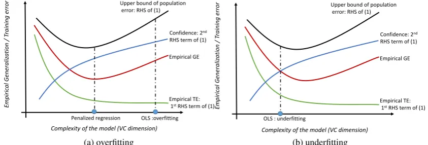
1. As shown in Figure 1, the RHS of eq. (2) establishes an upper bound for the population error

based on the eTE and the VC dimensionh. When the effective sample size for the training set (nt/h) is very large,εis very small, the second term on the RHS of (2) becomes small,

and the eTE is close to the population error. In this case the extremum estimator has a good

GA. However, if the effective sample sizent/his small (i.e., the model is very complicated),

the second term on the RHS of (2) becomes larger. In such situations a small eTE does not

guarantee a good GA, and overfitting becomes more likely.

2. The VC dimensionhis a more general measure of model complexity than the number of parameters, p, which does not readily extend to nonlinear or non-nested models. Whileh

reduces to pdirectly for generalized linear models,hcan also be used to partially order the complexity of nonlinear or non-nested models by summarizing their geometric complexity.7

Complexity of the model (VC dimension)

Upper bound of population error: RHS of (1)

Empirical GE

Empirical TE: 1st_{RHS term of (1)} Confidence: 2nd RHS term of (1)

E

mpi

ri

cal

Genera

li

zati

on

/ T

rai

n

ing

error

OLS :overfitting Penalized regression

(a) overfitting

Complexity of the model (VC dimension)

Upper bound of population error: RHS of (1)

Empirical GE

Empirical TE: 1st_{RHS term of (1)}

Confidence: 2nd

RHS term of (1)

E

mpi

ri

cal

Genera

li

zati

on

/ T

rai

n

ing

error

OLS : underfitting

(b) underfitting

Figure 1: The VC inequality and eGE

As a result, eq. (2) can be implemented as a tool for both nonlinear and non-nested model

selection.

3. Eq. (2) can be generalized to non-i.i.d. cases. While the VC inequality focuses on the

relation between the population error and the eTE in the i.i.d. case, McDonald et al. (2011)

generalizes the VC inequality forα- andβ-mixing stationery time series while Smale and Zhou (2009) generalizes the VC inequality for panel data. Moreover, Michalski and Yashin

(1986); Skrondal and Rabe-Hesketh (2004); Wang and Feng (2005); Yu and Joachims (2009);

Pearl (2015) show that heterogeneity can be controlled by implementing the latent variable model or by adding the variable causing heterogeneity into the model, implying eq. (2) is

valid.

Based on the VC inequality, Vapnik and Chervonenkis (1971a) propose that minimizing the

RHS of (2), the upper bound of the population error, reduces overfitting and improves the GA of

the extremum estimator. However, this may be hard to implement because it can be difficult to calculate the VC dimension for anything other than linear models. In practice, statisticians have

implemented GA analysis by minimizing the eGE using validation or cross-validation. For example, cross-validation is used to implement many penalty methods, such as the lasso-type estimators,

ridge regression or bridge estimators. Clearly, however, the eGE and the population error are not

the same thing. Thus, the properties of the minimum eGE, such as its variance, consistency and convergence rate are of particular interest in the present context. By adapting and modifying eq. (2),

we propose the following inequalities that analyze the relation between the eGE and the eTE in

finite samples.

Theorem 2.1(The upper bound of the finite-sample eGE for the extremum estimator). UnderA1to

A3, the following upper bound for the eGE holds with probability at leastϖ(1₋1/nt),∀ϖ∈(0,1).

R_n

s(btrain|Ys,Xs)6

R_n

t(btrain|Yt,Xt)

(1₋√ε) +ς, (3)

whereR_n

s(btrain|Ys,Xs)is the eGE andRnt(btrain|Yt,Xt)the eTE for the extremum estimator btrain,

εis defined in Lemma 2.1,

ς =

      

     

ν

√

2τ(E_{[Q(btrain|Ys,Xs)])/(}√ν₁

−ϖ_·ns1−1/ν) ifν∈(1,2]

B nsln

p

2/(1₋ϖ) if Q(_·)_∈(0,B]and B is bounded

var[Q(btrain|y,x)]/(n(1−ϖ)) ifν∈(2,∞)

and

τ>sup[

R

(Q(b_|y,x))νdF(y,x)]1/ν R

Q(b_|y,x)dF(y,x) .

A few comments follow from Theorem 2.1.

• (Upper bound of the finite-sample GA) eq. (3) establishes the upper bound of the eGE from any out-of-sample data of sizensbased on the eTE from any in-sample data of sizent. Unlike

the classical bound in Lemma 2.1, which captures the relation between the population error and the eTE, eq. (3) establishes inequalities to quantify the upper bound of the finite sample

eGE. Usually, we need to use validation or cross-validation to measure the eGE of a model

with new data. However, because the RHS of eq. (3) is directly computable it may be used as a measure of finite-sample eGE, avoiding the need for validation.

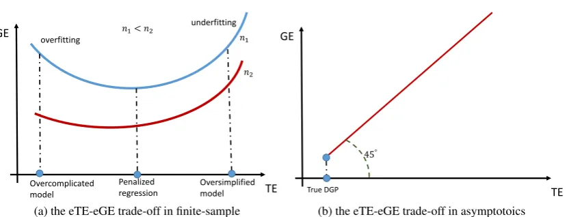
• (The eGE-eTE trade-off in model selection) eq. (3) also characterizes the trade-off between eGE and eTE for model selection in both the finite sample and asymptotic cases. In Figure 2b,

the population eGE, population eTE and population error are expected to be identical in

asymptotic case. Hence, minimizing eTE can directly lead to the true DGP in the population. In contrast, as illustrated in Figure 2a, in finite samples, an overcomplicated model with

lownt/hwould have a small eTE for the data whereas eq. (3) show that the upper bound

of the eGE on new data will be large. Hence, the overcomplicated model willoverfit the in-sample data and typically have a poor GA. In contrast, an oversimplified model with high

nt/h, typically cannot adequately recover the DGP and the upper bound of the eGE will also

be large. As a result, the oversimplified model willunderfit, fitting both the in-sample and out-of-sample data poorly. Thus, the complexity of a model introduces a trade-off between

the eTE and eGE in model selection.

• (GA and distribution tails) eq. (3) also shows how the tail of the error distribution affects the upper bound of the eGE. If the loss distributionQ(_·)is bounded or light-tailed, the second term of eq. (3),ς, is mathematically simple and converges to zero at the rate 1/ns. If the loss

GE

TE

underfitting

Overcomplicated model

Penalized regression overfitting

Oversimplified model

𝑛1

𝑛2 𝑛1< 𝑛2

(a) the eTE-eGE trade-off in finite-sample

GE

TE 45°

True DGP

(b) the eTE-eGE trade-off in asymptotoics

Figure 2: Schematic diagram of the trade-off between eGE and eTE

that is a closed-form for the loss distribution,8can be used to measure the heaviness of the

loss distribution tail, a smaller ν implying a heavier tail. In the case of a heavy tail, the second term of eq. (3),ς, becomes mathematically complicated and its convergence rate

decreases to 1/n1s−1/ν. Hence, eq. (3) shows that the heavier the tail of the loss distribution,

the higher the upper bound of the eGE and the harder it is to control GA in finite samples. In the extreme case withν=1, there is no way to adapt eq. (3).

Essentially, validation randomly partitions the data into a training set and a test set, yielding an estimate on the training set that is used to compute the eGE of the test set. Eq. (3) measures the

upper bound the eGE on the test set from the model estimated on the training set with a given eTE

andh. In other words, eq. (3) directly measure GA using validation. Furthermore, a similar bound to eq. (3) can be established forK-fold cross-validation.

Theorem 2.2 (The upper bound of the finite-sample eGE for the extremum estimator under

cross-validation). UnderA1toA3, the following upper bound for the eGE holds with probability at leastϖ(1₋1/K),_∀ϖ_∈(0,1).

1

K

K

∑

j=1

R_n

s(btrain|Y

j s,Xsj)6

1

K∑

K

q=1Rnt(btrain|Y

q t ,X

q t )

(1₋√ε) +ςcv, (4)

whereR_n

s(btrain|Y

j

s,Xsj)is the eGE of btrainin jth round of validations,Rnt(btrain|Y

q t ,X

q t )is the

eTE of btrainin qth round of validations, and

ςcv=

            

ν

√

2τR_{(btrain|Y,X)/(}√ν

1₋ϖ_·ns1−1/ν) ifν∈(1,2]

Blnp2/(1₋ϖ)/ns if Q(·)∈(0,B]and B is bounded

var[Q(btrain|y,x)]/(n2s(1−ϖ)) ifν∈(2,∞)

8_{It is closed-form because owing toA1, which guarantees closed-form, first-order moments for all loss distribution in}

The errors generated by cross-validation are affected both by sampling randomness from the population and by sub-sampling randomness that arises from partitioning the sample into folds.

Thus, the errors from cross-validation are potentially more volatile than the usual errors from

estimation. Theorem 2.2 provides an upper bound for the average eGE under cross-validation, which offers a way to characterize the effect of sub-sampling randomness and suggests a method to

approximate the GA from cross-validation. The following comments summarize the implications

of eq. (4).

1. (The upper bound of the eGE) Similar to eq. (3), eq. (4) serves as the upper bound of the averaged eGE generated by cross-validation. Both equations show the eTE-eGE trade-off and reveal the effect of a heavy tail on GA.

2. (Tuning the cross-validation hyperparameter K) Eq. (4) characterizes how the hyperparameter

Kaffects the averaged eGE from cross-validation (also called the cross-validation error in the literature). As explained above, the random partitioning in cross-validation introduces

sub-sampling randomness. With a given sample and fixedK, sub-sampling randomness will produce a different averaged eGE each time cross-validation is performed. WhenKchanges, the size of each fold changes, implying the training and test sets also change. WhenKis large, the test sets become small, increasing sub-sampling randomness. WhenKis small, the training sets become small, increasing sub-sampling randomness. For extremum estimators like OLS, the bias-variance trade-off is straightforward to analyze for different pbecause the sample is fixed. In contrast, the sub-sampling randomness introduced by cross-validation, the bias-variance trade-off for averaged eGE of cross-validation cannot be studied with the

given training and test set whenKchanges. As a result, in order to characterize and control for the influence of sub-sampling randomness, we establish the bias-variance trade-off for cross-validation by its upper bound, after running cross validation multiple times, as is

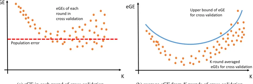
illustrated in Figure 3.

(a) (Large bias, small variance)WhenKis small,nt is smaller in each round of in-sample

estimation. Hence, as shown in Figure 3a, the eTE in each round,R_n

t(btrain|Y

q

t ,Xtq)/(1−

√

ε), is more biased from the population error. As shown in Figure 3b, theK-round averaged eTE, _K1∑K_q=1R_n

t(btrain|Y

q t ,X

q t )/(1−

√

ε), is more biased away from the true population error asKgets smaller. As a result, the RHS of eq. (4) suffers more from finite-sample bias. However, since small Kimplies that more data is used for eGE calculation in each round (nsis not very small), in each round the eGE on the test set

should not be very volatile. Thus, theK-round averaged eGE for cross-validation is not very volatile, which is shown by the fact thatςcvis not very large in eq. (4).

(b) (Small bias, large variance)WhenKis large,nsis small and the test set in each round

is small. Hence, with largeK, the eGE in each round may be hard to bound from above, which implies that the averaged eGE fromKrounds is more volatile. As a result,ςcv

tends to be large. However, with largeK, the RHS term_K1∑K_q=1R_n

t(btrain|Y

q t ,X

q t )/(1−

√

eGE

K eGEs of each

round in cross validation

Population error

(a) eGE in each round of cross-validation

eGE

K

K-round averaged eGEs for cross validation Upper bound of eGE

for cross validation

(b) average eGE fromKrounds of cross-validation

Figure 3: Representation of the bias-variance trade-off for cross-validation eGE

As shown in Figure 3b, the averaged eGE from cross-validation follows a typical

bias-variance trade-off by value ofK. IfKis small, the averaged eGE is computationally cheap and less volatile but more biased away from the population error. AsK gets larger, the averaged eGE becomes computationally expensive and more volatile but less biased away

from the population error. This result exactly matches the Kohavi et al. (1995) simulation study. More specifically, by tuning K to the lowest upper bound, we can find theK that maximizes the GA from cross-validation.

Theorems 2.1 and 2.2 establish the finite-sample and asymptotic properties of GA analysis

for any extremum estimator. In finite-sample analysis, the results capture the trade-off between eGE and eTE, which can be used to measure the GA of an econometric model. In asymptotic

analysis, eGE minimization is consistent. As a result, GA can be implemented as a criterion for

model selection, and directly connects to the theoretical properties for model selection methods such as penalized extremum estimation, the various information criteria and maximum a posteriori

(MAP) estimation. Minimizing eGE works especially well for penalized regression. As shown in

Algorithm 1, penalized regression estimation returns abλ for eachλ. Each value ofλ generates a

different model and a different eGE. Intuitively, Theorems 2.1 and 2.2 guarantee that the model

with the minimum eGE from_{b_λ}has the best empirical generalization ability. In the next section, we study the finite-sample and asymptotic properties of eGE for all penalized regressions.

3. Finite-sample and asymptotic properties of eGE for penalized regression

Using the classical concentration inequalities in Section 2, we established the upper bound for

the finite-sample eGE of the extremum estimator given any random sample of any size. We also revealed the trade-off between eTE and eGE for model selection and derived the properties of eGE

under validation and cross-validation. In this section, we apply the framework and results from

3.1. Definition of penalized regression

Firstly, we formally define penalized regression and its two most popular variants: ridge

regression (L_{2-penalized regression) and the lasso (}L_{1-penalized regression).}

Definition 3.1(Penalized regression,L_{2-eGE and}L_2-eTE).

1. (General form) The general form of the objective function for penalized regression is as follows

min

bλ

1

n(kY−X bλk2)

2

+λPenalty(_kb_λkγ). (5)

where Penalty(_{k · k}γ)stands for the penalty term, which is a function of theLγ norm of the

b_λ.

2. (b_λ and bpen) We denote bλ to be the solution of eq. (5) given the value of the penalty

parameter λ while bpen is defined to be the model with the minimum eGE among all

alternative_{b_λ}, as in Algorithm 1 in Section 1.

3. (Lasso and ridge) The objective functions for lasso (L_{1penalty) and ridge regression (}L₂ penalty), respectively, are

min

bλ

1

n(kY−X bλk2)

2₊

λkbλk1, (6)

and

min

bλ

1

n(kY−X bλk2)

2

+λ_kbλk2. (7)

4. (L_{2error for regression)the eTE and eGE for regression are defined in}L_{2form respectively} as follows:

R_n

t(btrain|Yt,Xt) =

1

nt k

Yt−Xtbtraink22

R_n

s(btrain|Ys,Xs) =

1

nsk

Ys−Xsbtraink22

The idea behind penalized regression is illustrated in Figure 4 wherebλ refers to the penalized

regression estimates for someλ and bOLS refers to the OLS estimates. As shown in Figure 4a,

differentL_{γ norms correspond to different boundaries for the estimation feasible set. For the}L₁

penalized regression (lasso), the feasible set is a diamond since each coefficient is equally penalized by theL_{1norm. The feasible area shrinks under a}L_{0.5penalty. Hence, as shown in Figure 4a,}

given the sameλ, the smaller isγ, the more likelyb_λ is to be a corner solution. Hence, given the sameλ, under theL_{0.5penalty variables are more likely to be dropped than with the}L_1orL₂ penalty.9 In special cases whenγ=0 andλ is fixed at 2 (lnnt), theL0penalized regression is

identical to the Akaike (Bayesian) information criterion.

9_{For 0<γ<1, the penalized regression may be a non-convex programming problem. While general algorithms have}

not been found for non-convex optimization, Strongin and Sergeyev (2013), Yan and Ma (2001) and Noor (2008) have

developed functioning algorithms. Forγ=0, the penalized regression becomes a discrete programming problem, which

𝑏2

𝑏1 𝐿∞ 𝐿2 𝐿1 𝐿0.5

(a) boundaries forL_0,L_0.5,L_1,L_2and

L_∞penalties

𝑏2

𝑏1 𝑏𝑂𝐿𝑆

𝑏𝜆 Level sets of 𝐿2error

(b)L_{1penality (lasso)}

𝑏2

𝑏1

𝑏𝑂𝐿𝑆

𝑏𝜆

(c)L_0.5penality

Figure 4: Illustration of various penalized regressions

The last important comment is that penalized regression primarily focuses on overfitting. By contrast, OLS minimizes the eTE without any penalty, typically causing a large eGE (as shown in

Figure 1a). There is also the possibility that OLS predicts the data poorly, causing both the eTE

and eGE to be large. The latter refers to underfitting and is shown in Figure 1b. We are more capable of dealing with overfitting than underfitting despite the fact that it possible to quantify GA

or the eGE.10Typically overfitting in OLS is caused by including too many variables, which we can

resolve by reducingp. However, underfitting in OLS is typically due to a lack of data (variables) and the only remedy is to collect additional relevant variables.

3.2. Schematics and assumptions for eGE minimization with penalized regression

As shown in Section 2, eGE minimization improves finite-sample GA, implying the estimator has a lower eGE on out-of-sample data. In this section, we implement the schematics of eGE

minimization on penalized regression. We demonstrate: (1) specific error bounds for any penalized

regression, (2) a generalL_{2consistency property for penalized regression estimates, (3) that the} upper bound for theL_{2difference betweenbpenandbOLSis a function of the eGE, the tail property} of the loss distribution and sample exogeneity.

The classic route to derive asymptotic or finite-sample properties for regression is through analyzing the properties of the estimate in the space of the eTE. In contrast, to study how penalized

regression improves GA or eGE and balances the in-sample and out-of-sample fit, we reformulate

the asymptotic and finite-sample problems in the space of the eGE. We show that, under the framework of eGE minimization, a number of finite-sample properties of penalized regression can

be explained by eGE or the finite-sample GA.

In asymptotic analysis, consistency is typically considered to be one of the most fundamental properties. To ensure that eGE minimization is a reliable estimation approach, we prove that the

penalized regression, which is a specific form of the eGE minimizer, converges to the true DGP as

Λ: a `class’ of

models, where true DGP 𝛽exists

True DGP

Space of eGE Space of models

𝒃𝒑𝒆𝒏

Finite sample

Asymptotic

Minimal eGE among all other

alternative 𝑏_𝜆

Theorem 2

Minimal population GE

Proposition 1 OLS: eTE

minimizer

Figure 5: Outline of proof strategy

n_→∞. Essentially, we show that penalized regression bijectively mapsbpento the minimal eGE

among_{bλ}on the test set. To bridge between the finite sample and asymptotic results we need to

show that if

• the true DGPβ is bijectively assigned to the minimal eGE in population, and

• minb∈bλ 1

ns∑

ns

i=1kYs−Xsbk22→minb

R

ky₋xTb_k22dF(y,x),

thenbpenis consistent in probability orL2, or

bpen=argmin{eGEs of{bλ}}

PorL₂

→ argmin

b

Z

kys−xTsbk22dF(y,x) =β.

At the outset, we stress that each variable in(Y,X)must be standardized before implementing penalized regression. Without standardization, as shown by (Tibshirani, 1996), the penalized

regression may be influenced by the magnitude (units) of the variables. After standardization, of

course,X andY are unit- and scale-free.

To ensure the consistency of penalized regression, we require the following three additional

assumptions.

Further assumptions

A4. The true DGP isY=Xβ+u. A5. E _uT_X=0.

A6. No perfect collinearity inX.

The assumptions A4to A6restrict the true DGPβ to be identifiable. Otherwise, there might exist another model that is not statistically different from the true DGP. The assumptions are quite

3.3. Necessary propositions for final results

Under assumptionsA1toA6, we show that the true DGP is the most generalizable model,

yielding Proposition 3.1.

Proposition 3.1(Identification ofβ in the space of eGE). Under assumptionsA1toA6, the true DGP, Y =Xβ+u, is the one and only one offering the minimal eGE asen_→∞_.

Proposition 3.1 states that there is a bijective mapping betweenβ and the global minimum eGE

in the population. IfA5orA6are violated, there may exist variables in the sample that render the true DGP not to be the model with minimum eGE in population. As shown in Algorithm 1,

penalized regression picks the model with the minimum eGE in_{b_λ}to bebpen. As a result, we

also need to prove that, when the sample size is large enough, the true DGP is included in_{bλ}, the

list of models from which validation or cross-validation selects. This is shown in Proposition 3.2.

Proposition 3.2(Existence ofL_{2consistency). Under assumptionsA1toA6and Proposition 3.1,}

there exists at least oneeλ such thatlim_en→∞kb_eλ−βk2=0.

𝑏2

𝑏1

𝑏𝑂𝐿𝑆

𝑏𝜆

𝛽

(a) under-shrinkage

𝑏2

𝑏1

𝑏𝑂𝐿𝑆

𝑏𝜆

𝛽

(b) perfect shrinkage

𝑏2

𝑏1

𝑏𝑂𝐿𝑆

𝑏𝜆

𝛽

(c) over-shrinkage

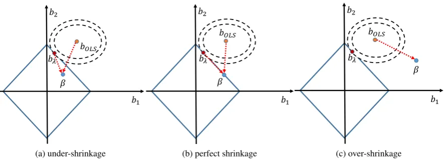
Figure 6: Various types of shrinkage under anL_1penalty

Since the penalized regression can be sketched as a constrained minimization of the empirical

error, we can illustrate Proposition 3.1 and 3.2 in Figure 6 using lasso as the example of a penalized regression. In Figure 6, the parallelogram-shaped feasible sets are determined by theL_{γ penalty,}

b_λ refers to the solution of eq. (5),β refers to the true DGP, andbOLSrefers to the OLS estimates.

Different values forλ imply different areas for the feasible set of the constrained minimization; the area of the feasible set gets smaller as the value ofλ gets larger. Hence, one of three cases may

occur: (i) as shown in Figure 6a, for a small value ofλ,β lies in the feasible set (under-shrinkage)

and offers the minimum eTE in the population; (ii) as shown in Figure 6b, for the oracleλ,β is located precisely on the boundary of the feasible set (perfect-shrinkage) and still offers the

minimum eTE in the population; (iii) as shown in Figure 6c, for a large value ofλ,β lies outside

the feasible set (over-shrinkage). In cases (i) and (ii), the constraints become inactive asne_→∞, so lim_en→∞bλ =limne→∞bOLS =β. However, in case (iii), limne→∞bλ6=β. Therefore, tuning the

3.4. Main results for penalized regression estimates

As shown above, intuitively the penalized regression estimate is expected be consistent in some

norm or measure as long as we can be sure that for a specificλ,β lies in the feasible set and offers the minimum eTE in population. However, in practice we may not know a priori whichλ causes

over-shrinkage and which does not, especially when the number of variables,p, is not fixed. As a result, we need to a method such as cross-validation or validation to tune the value ofλ. Thus,

as a direct application of eGE minimization in Section 2, we use GA/eGE analysis to show that

eGE minimization guarantees the model selected by penalized regression,bpen, asymptotically

converges inL_{2to the true DGP.}

In the following section we analyze the finite-sample and asymptotic properties of the penalized

regression estimate in two scenarios:n>pandn<p. In the case wheren>p, OLS is feasible, so we take the OLS estimate for the unpenalized regression estimate. However, whenn<p, OLS is not feasible, and we use forward stagewise regression (FSR) for the unpenalized regression

estimate. Hereafter,bOLSis the OLS estimate from the training set.

3.4.1. Case: n>p

Firstly, by specifying eq. (3) and (4) in the context of regression, we can establish the upper

bound of the eGE, as shown in Lemma 3.1.

Lemma 3.1(Upper bound of the eGE for the OLS estimate). UnderA1 to A6, if we assume u_∼Gaussian(0,var(u)),

1. (Validation) The following bound for the eGE holds with probability at leastϖ(1₋1/nt)for

bOLS,∀ϖ∈(0,1).

1

ns

(_kesk2)26

(_ketk2)2

nt(1−√ε)

+2(var(u)) 2

ns√1−ϖ

, (8)

where esis the OLS eGE, et is the OLS eTE, andεis defined in Lemma 2.1.

2. (K-fold cross-validation) The following bound for the eGE holds with probability at least

ϖ(1₋1/K)for bOLS,∀ϖ∈(0,1).

1

K

K

∑

j=1

(_kesjk2)2

n/K 6

n(K₋1)∑K_q=1(_ketqk2)2

K2₍₁₋√_ε) +

2(var(u))2

√

1₋ϖ_·(n/K)2, (9)

where esjis the eGE of OLS estimate in the jth round, eqt is the eTE of OLS in the qth round,

whileε andς are defined in Lemma 2.1.

Eq. (8) and (9) show that the higher the variance ofuin true DGP, the higher the upper bound of the eGE in validation and cross-validation. Based on eq. (9), the lowest upper bound of the

cross-validation eGE is determined by minimizing the expectation of the RHS of eq. (9), yielding

Corollary 3.1 (The optimal K for penalized regression). Under A1 to A6 and eq. (9) from Lemma 3.1, if we assume the OLS error term u_∼Gaussian(0,var(u)), the optimal K for cross-validation in regression (the minimum expected upper bound of eGE) is defined:

K∗=argmin

K

var(u)

1₋√ε+

4(var(u))2

√

1₋ϖ(n/K)2

Similar to eq. (3), eq. (8) and (9) respectively measure the upper bound of the eGE for the

OLS estimate using validation and cross-validation. In standard practice, neither validation nor

cross-validation are implemented as part of OLS estimation and hence the eGE of the OLS estimate is rarely computed. Eq. (8) and (9) show that eGE can be computed without having to carry out

validation or cross-validation.

In penalized regression, the penalty parameterλ can be tuned by validation orK-fold cross-validation. ForK>2, we haveKdifferent test sets for tuningλ andKdifferent training sets for estimation. Based on eq. (8) and (9), an upper bound for theL_{2predicted difference betweenbOLS} andbpencan be established under validation and cross-validation, as shown below.

Proposition 3.3(L_{2distance between the penalized and unpenalized predicted values). UnderA1}

toA6and based on Lemma 3.1, Proposition 3.1, and Proposition 3.2,

1. (Validation) The following bound holds for the validated bpenwith probabilityϖ(1−1/nt)

1

ns

(_kXsbOLS−X bpenk2)26

1

nt

ketk22

1₋√ε− 1

nsk

esk22

+ 4

nsk

eT_sXsk∞kbOLSk1+ς (10)

whereς is defined in Lemma 3.1.

2. (K-fold cross validation) The following bound holds for the K-fold cross-validated bpenwith

probabilityϖ(1₋1/nt)

1

K

K

∑

q=1

1

ns

(_kX_sqbq_OLS−X_sqbq_penk2)2 6

1 nt 1 K∑ K q=1

eq_t2₂

1₋√ε −

1

K

K

∑

q=1

1

nsk

eq_sk2₂ (11) + 1 K K

∑

q=1

4

ns

(eq_s)TX_sq

_∞bq_OLS1+ςcv.

where eqt is the eTE of the OLS estimate in the qth round of cross-validation, e q

s is the eGE of

the OLS estimate in the q round of cross-validation and bq_OLS is the OLS estimate in the qth round of cross-validation.

We can now derive the upper bound of_kbOLS−bpenk2, as shown in Theorem 3.1.

Theorem 3.1(L_{2distance between the penalized and unpenalized estimates). UnderA1toA6}

and based on Propositions 3.1, 3.2, and 3.3,

1. (Validation) The following bound holds with probabilityϖ(1₋1/nt):

kbOLS−bpenk26

s

1 ρnt

ketk22 (1₋√ε)−

1 ρnsk

esk2₂

+ s 4 ρnsk

eT

sXsk∞kbOLSk1+

whereρis the minimal eigenvalue of XTX andς is defined in Lemma 3.1.

2. (K-fold cross validation) The following bound holds with probabilityϖ(1₋1/nt):

1

K

K

∑

q=1

(_kbq_OLS−bq_penk2)2 6

K1∑

K q=1nt1·ρ

keqtk

2 2

1−√ε −

1

K∑

K q=1ns·1ρ¯

eqs

2

2

+_K1∑K_q=1n4

s·ρ¯

(eqs)TXsq

_∞bq_OLS1+_ρς_¯ (13)

whereρ¯ is defined asmin

n

ρq|ρqis the minimal eigenvalue of Xsq

T

Xsq,∀q

o .

Some important remarks apply to Theorem 3.1. The LHS of eq. (12) essentially measures how

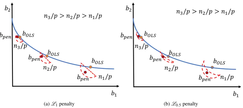
much the penalized regression estimate differs from the OLS estimate under validation. The RHS of eq. (12) essentially captures the maximumL_{2difference betweenbOLSandbpen. As shown in} eq. (12), the maximum difference depends on the GA of the true DGP and the GA of the OLS model in several different forms.

• The first term on the RHS of eq. (12) (ignoring 1/ρ) is the difference between the eGE from OLS and the upper bound of the population error for the OLS estimate, or, equivalently,how far the GA of the OLS estimate is from its maximum. The larger the GA ofbOLS, the less

overfitting OLS generates, the closer the eGE ofbOLSis to the upper bound of the population

error, and the smaller the first term on the RHS of eq. (12).

• The second term on the RHS of eq. (12) (ignoring 4/ρ) measures the empirical endogeneity of the error term of the OLS estimate on the test set. On the training seteT_t Xs=0, but in general

eT_sXs6=0 on the test set. Hence, _n1_skeTsXsk∞kbOLSk1 measures the GA for the empirical

moment condition of the OLS estimate on out-of-sample data.11 The more generalizable the OLS estimate, the closereT

sXsis to zero on out-of-sample data, and the smaller the second

term on the RHS of eq. (12).

• The third term on the RHS of eq. (12) is affected byς, whichmeasures the heaviness of the tail in the loss distribution for the OLS estimate. Similar to the comments of Theorem 2.1, the OLS loss distribution affects the GA of the OLS estimate. The heavier the loss tail, the

more volatile the eGE on out-of-sample data, and the more difficult it is to bound the eGE

for OLS.

• All three RHS terms in eq. (12) are affected byρ, the minimum eigenvalue ofX_xTXs, which

can be thought of as a measure of the curvature of the objective function for penalized regression. The larger the minimum eigenvalue, the more convex the objective function. Put another way, it is easier to identify the true DGPβ from the alternatives asnget larger.

The interpretation of eq. (13) is similar to eq. (12) adjusting for cross-validation. Hence, the

first term on the RHS of eq. (13) (ignoring 1/ρ) stands for how far away theaverageGA of OLS

11_{Because we standardize the test and training data, the moment conditionE(e}

𝑏𝑂𝐿𝑆

𝑏𝑝𝑒𝑛 𝑏2

𝑏1 𝑏𝑂𝐿𝑆

𝑏𝑝𝑒𝑛 𝑏𝑝𝑒𝑛 𝑏𝑂𝐿𝑆

𝑛1/𝑝 𝑛2/𝑝

𝑛3/𝑝

𝑛3/𝑝 > 𝑛2/𝑝 > 𝑛1/𝑝

(a)L_1penalty

𝑏𝑂𝐿𝑆

𝑏𝑝𝑒𝑛 𝑏2

𝑏1 𝑏𝑂𝐿𝑆

𝑏𝑝𝑒𝑛 𝑏𝑝𝑒𝑛 𝑏𝑂𝐿𝑆

𝑛1/𝑝 𝑛2/𝑝

𝑛3/𝑝

𝑛3/𝑝 > 𝑛2/𝑝 > 𝑛1/𝑝

(b)L_0.5penalty

Figure 7: Illustration of the relation betweenbOLSandbpen

estimate is from its maximum inKrounds of validation. The second term on the RHS of eq. (13) (ignoring 4/ρ) indicateson averagehow generalizable the empirical moment condition of the OLS estimate is with out-of-sample data inKrounds of validation. Similarly,ς indicateson average

the heaviness in the tail of the loss distribution inKrounds of validation. As a direct result of Theorem 3.1, theL_{2consistency for the penalized regression estimate is established as follows.}

Corollary 3.2(L_{2consistency for the penalized regression estimate whenn>p). UnderA1to}

A6and Propositions 3.1, 3.2, and 3.3, if we assume the error term u_∼Gaussian(0,var(u)), then bpenconverges in theL2norm to the true DGP if limn_→∞p/ne=0

Theorem 3.1 and Corollary 3.2 are illustrated in Figure 7. Typically, due to the poor GA of the

OLS estimate, the penalized regression estimatebpenwill not lie on the same convergence path as

the OLS estimate. However, Theorem 3.1 shows that the deviation ofbpenfrom the convergence

path is bounded. Furthermore,bpentypically lies within anε-ball centered onbOLSwhose radius is

a function of the eGEs of the OLS estimate and the true DGP. Also, as shown in Figures 6a and 6b,

bpenalways lies within the feasible set parameterized byλkbkγ. Hence, as shown in Figures 7a and

7b,bpentypically is located in the small area at the intersection of theLγ feasible area andε-ball.

Unless the optimalλ from validation or cross-validation is 0, the OLS estimate will never be in the

feasible area of the penalized regression estimate, which is why the intersection region is always

below thebOLS. Asn/pincreases, theε-ball becomes smaller, the penalized regression estimate

gets closer to the OLS estimate, and both converge toβ.

3.4.2. Case: n<p

Typically, to ensurebOLS can identify the true DGPβ, we require that(kek2)2 is strongly

convex, or that the minimal eigenvalue ofXTX, ρ, is strictly larger than 0. However, if p>n, ρ=0 and the space of(_ke_k2)2is flat in some direction. As a result, thekbOLSk1is not closed-form,

the true DGPβ cannot be identified and Eqs. (12) and (13) are trivial.

Put another way, we need to ensure that the strong convexity of the space(_ke_k2)2is still reserved

for thep>ncase andβ is still identifiable. This is guaranteed by the sparse eigenvalue condition (Bickel et al., 2009; Meinshausen and Yu, 2009; Zhang, 2010)—see the proof of Proposition 3.4

(below) in Appendix 1 for the details.

Regression can at most estimate max(p,n)coefficients. When p>n, penalized regression has to drop some variables to make it estimable, implying thatγ>1 does not apply to thep>ncase. Hence, for thep>ncase, we focus only on theL_{1penalized regression, i.e., the lasso. As shown} by Efron et al. (2004); Zhang (2010), lasso may be thought of as a forward stagewise regression

(FSR) with anL_{1norm constraint.}12 _{Hence, lasso regression can be treated as a form of GA/eGE}

control for FSR whenp>n. As shown by Zhang (2010), even though FSR is a greedy algorithm that may result in overfitting in finite samples, it is stillL_{2consistent under the sparse eigenvalue}

condition

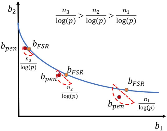
Thus, forp>n, we set the FSR estimate,bFSR, to be the unpenalized regression estimate, and

theL_{1penalized regression estimate,bpen, to be the penalized regression estimate. In} Proposi-tion 3.4 and Corollary 3.3, we show that the lasso preserves the properties and interpretaProposi-tions of the

n>pcase by reducing the overfitting inherent in FSR.

Proposition 3.4(L_{2distance between the}L_{1penalized and unpenalized FSR estimates). Under}

A1toA6and based on Lemma 3.1, Propositions 3.1, and 3.2 and the sparse eigenvalue condition,

1. (Validation) The following bound holds with probabilityϖ(1₋1/nt)

kbFSR−bpenk2 6

r ρre1nt

ketk22 (1−√ε)−

1

ρrenskesk 2 2

+q_ρ4 renske

T

sXsk∞kbFSRk1+

ς ρre 1 2 (14)

whereρreis the minimum of the sparse eigenvalues of XTX and bFSRis the FSR estimate.

2. (K-fold cross-validation) The following bound holds with probabilityϖ(1₋1/nt)

1

K

K

∑

q=1

bq_FSR−bq_pen2₂ 6

K1∑

K q=1nt·1ρ¯re

keqtk

2 2

1−√ε −

1

K∑

K q=1ns1·ρ¯re

eqs

2 2

+_K1∑K_q=1n4

s·ρ¯re

eqs

T

Xsq

_∞kbFSRk1+

ς

¯

ρre (15)

whereρ¯reis defined asmin

h

ρreq |ρreq is the minimal restricted eigenvalue of Xsq

T

Xsq,∀q

i

and bq_FSRis the FSR estimator in the qth round of valid