The employment effect of minimum wage using 77 international studies since 1992: A meta analysis

(1)

Munich Personal RePEc Archive

The employment effect of minimum wage

using 77 international studies since 1992:

A meta-analysis

Chletsos, Michael and Giotis, Georgios P.

University of Ioannina, Department of Economics, Greece

14 January 2015

(2)

The employment effect of minimum wage using 77 international studies since

1992: A meta-analysis

Michael Chletsos1and Georgios P. Giotis2

Abstract

Until the early 90’s a strong consensus existed among economists that minimum wage has negative employment effects. However, in 1992, the studies by Card (1992a) and Katz and Krueger (1992), who found insignificant and slightly positive effects, respectively, came to create a schism. Since then a divergence of views expressed by conflicting empirical studies exists in the literature. In our paper, we use a meta-sample of 77 international studies from 18 countries to investigate this relationship. Our analysis suggests that there is evidence of publication selection, but no effect of minimum wages on employment measures. Additionally, using 27

moderators as potential explanatory variables in order to explain the variation among studies, we find that study characteristics related to the data, the model specifications and the group concerned, diversify the degree of the effect.

JEL Classification: J38, J21, C12.

Keywords: Minimum wage, Employment, Meta-analysis.

1_{Corresponding author at: University of Ioannina, Department of Economics, P.O. Box 1186, 45110}

Ioannina, Greece. Tel.: +30 2651005924, Fax: +30 2651005092, E-mail address: [email protected].

2_{University of Ioannina, Department of Economics, P.O. Box 1186, 45110 Ioannina, Greece. Tel.: +30}

(3)

1. Introduction

Until the early 90’s a strong consensus existed among economists that an increase in the minimum wage would cause an increase in unemployment. This neoclassical approach was the prevailing theory in labor economics and the studies that were conducted to investigate this relationship used basically time-series data. However, at the beginning of 90’s the studies by Card (1992a) and Katz and Krueger (1992) came to create a schism as they didn’t find evidence of adverse employment effects of minimum wages. Since then, a divergence of views exists in the literature, which is expressed by conflicting empirical studies.

In this frame of opposing results triggered by Card, Katz and Krueger, it seemed quite interesting to us to approach this issue with meta-analysis techniques, which are very useful statistical tools for reviewing empirical results. In our research, we found seven studies that use meta-analysis methods to investigate the employment

effects of minimum wages, and remarkable is the fact that apart from two studies, conducted by Boockmann (2010) and Belman and Wolfson (2014), no other study uses worldwide studies as a meta-sample.

In general, we would say that the scientific work on the employment effect of minimum wages using meta-analysis methods, usually deals with USA studies or a homogeneous group of countries. Concisely, it seemed intriguing to approach this issue using meta-analysis techniques with studies from all over the world. In our analysis we found that there is evidence of publication selection, but no effect of minimum wages on employment measures. In addition, using 27 moderators as potential explanatory variables in order to explain the variation among studies, we found that study characteristics related to the data, the model specifications and the group concerned, diversify the degree of the effect. This conclusion is drawn from a meta-sample of 77 studies from 18 countries, which provided 1.521 elasticities with their standard errors or t-statistics.

2. Review of meta-analysis literature on the employment effect of minimum

wage

(4)

found publication bias in favor of studies that provided a statistically significant negative employment effect. All the studies which the authors used as a meta-sample were conducted for the USA and the structure of the data was time-series. Card and Krueger suggested that later studies, which had more data and lower standard errors, did not show the expected increase in t-statistic (almost all the studies had a t-statistic of about two, just above the level of statistical significance at the 5%). Card and Krueger’s study created a schism among economists by providing evidence that minimum wage increases did not decrease employment.

The second meta-analysis on the employment effect of minimum wages is found 14 years later, in 2009, when Hristos Doucouliagos and Tom D. Stanley conducted a similar meta-analysis of 64 U.S. studies that offered 1.474 estimates of the employment elasticity and concluded that Card and Krueger’s initial claim of publication bias was still correct. Moreover, they concluded that once this publication selection was corrected, an adverse employment effect was not supported by this large

and rich research record on the employment effects of minimum-wage regulation. That study had an important impact on the economic research with the use of meta-analysis techniques and boosted the meta-meta-analysis studies in economics.

Thirdly, Boockmann (2010) conducted a meta-analysis of 55 empirical studies estimating the employment effects of minimum wages in 15 industrial countries since 1995. Almost 67% of the estimations of the meta-sample provided negative signs of the impact of minimum wages on employment. The results were in line with theoretical expectations of the neoclassical theory the degree to which they were robust differed across institutions of the countries, though. That study is the first study which used a sample of international studies and not for a single country, and it incorporated three particular labor market regulations as possible sources of policy complementarities to explain differences between the countries (the benefit replacement ratio, the employment protection and the collective bargaining system).

(5)

caution researchers from applying widely used estimators, such as random effects weighted averages and random-effects MRA models, to econometrics estimates’.

The last three studies that have used meta-analysis techniques to investigate the employment impact of minimum wages were published in 2014. The first one was conducted by Nataraj, Perez-Arce, Srinivasan and Kumar (2014), on low-income-countries. Their meta-sample included fifteen studies from individual countries and two cross-country studies, and the results showed an ambiguous effect of minimum wages on total employment as a total outcome of positive impact on informal employment and negative on formal employment.

The second study earlier in the year was conducted by Leonard, Stanley and Doucouliagos (2014). The authors used meta-analysis methods to investigate the effect of increases in the UK minimum wage on employment using studies conducted for the United Kingdom alone. The meta-sample consisted of 16 studies which provided 710 partial correlations and 236 elasticities and according to the results no

adverse effect of minimum wage could be found by the increases of the UK minimum wages apart from the residential home-care sector. In comparison to Doucouliagos and Stanley (2009), this study did not find evidence or publication bias as the larger US study does. Nevertheless, both studies practically indicated absence of significant adverse employment effect of minimum wages.

Finally, we would refer to Belman and Wolfson (2014) who used data from 23 international studies since 2000. The meta-sample provided 439 estimations and the majority of the studies concerned the USA. Generally, we could say that the authors found negative and statistically significant effects of minimum wage which were very small, though. The largest reliable employment elasticities were about -0.07 and the smallest -0.04 (youth employment) and -0.01 (in the food & drinking sector).

(6)

3. The meta-sample

The process of the identification of the studies which constitute the meta-sample is the first but very important step in the meta-analysis. We began our research using the search machine Google Scholar, and afterwards the economic databases Econlit, Sciencedirect, RePEc and Jstor. Mainly the keywords used in the search were “minimum wage” and “employment” and we used and other several flections as a keyword. Before entering into the details of the identification, it has to be pointed out that we restricted the research only to those studies published since 1992 which is the year when the studies by Card (1992a) and Katz and Krueger (1992), made the economic thinking reconsider the relationship, as until then a strong consensus existed which accepted that minimum wages had negative effect on employment.

Concerning the identification of the studies, our objective was to find those studies which investigate the effect of minimum wage on employment measures but not on unemployment or other measures, such as labor force participation rates.

Furthermore, we had to exclude from our meta-sample the studies which did not mention a direct minimum wage effect. For example, some of the studies reported estimations of the impact of wages generally on employment or, in other cases, the effect of distribution of income on employment measures. In addition to this, we followed Doucouliagos and Stanley (2009) and our analysis focuses on employment elasticities drawn from studies using a continuous measure of employment or hours. Moreover, we excluded those studies which use a binary dependent variable, reporting employment probabilities. However, in this way, many studies were excluded but we kept the meta-sample more homogeneous.

Another aspect which has to be mentioned is that we chose elasticities as size effects which has some disadvantages, as there are many studies that report only partial correlation coefficients, and if the calculation of the elasticities was not possible, it was another reason for exclusion. However, as Doucouliagos and Stanley (2009) refer at p. 412, the choice of elasticities as the common metric to measure the employment effect, is considered more appropriate, since they are often assumed to be relatively stable parameters. Furthermore, we excluded those studies which did not report standard errors or t-statistics which are both needed for publication selection bias correction.

(7)

which investigate the effect of minimum wages on employment measures or hours worked. The studies which are included in the meta-sample are presented in table A.1 at the appendix, by country, with a brief reference of the structure of the data used to obtain the elasticities. In addition to this, we present the studies that were dropped out of the meta-sample with the reason for exclusion in table A.2. The 77 studies of the meta-sample provided 1.521 elasticities with their standard errors or t-statistics.

(8)

[image:8.595.16.596.87.766.2]

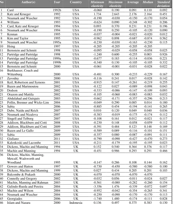
Table 1. Summary statistics of the studies in the meta-sample, by country.

No Author(s) Year Country Minimum

elasticity

Maximum elasticity

Average Median Standard deviation

1 Card 1992b USA -0.060 0.190 0.091 0.110 0.092

2 Katz and Krueger 1992 USA 1.734 2.643 2.176 2.164 0.451 3 Neumark and Wascher 1992 USA -0.190 -0.030 -0.150 -0.170 0.054

4 Williams 1993 USA -0.624 0.090 -0.248 -0.302 0.206

5 Card, Katz and Krueger 1994 USA 0.093 0.370 0.231 0.231 0.196 6 Neumark and Wascher 1994 USA -0.190 0.250 -0.105 -0.120 0.090

7 Kennan 1995 USA -0.037 -0.004 -0.021 -0.020 0.012

8 Kim and Taylor 1995 USA -0.962 0.898 -0.687 -0.874 0.562 9 Neumark and Wascher 1995a USA -0.230 -0.030 -0.163 -0.230 0.115

10 Hsing 1997 USA -0.205 -0.205 -0.205 -0.205

11 Bernstein and Schmitt 1998 USA -0.095 -0.029 -0.058 -0.058 0.025 12 Partridge and Partridge 1998 USA -1.240 0.600 -0.255 0.003 0.926 13 Partridge and Partridge 1999a USA -0.677 0.183 -0.114 -0.036 0.221 14 Partridge and Partridge 1999b USA -0.340 0.130 -0.105 -0.105 0.332 15 Bernstein and Schmitt 2000 USA -0.061 -0.001 -0.031 -0.028 0.022 16 Burkhauser, Couch and

Wittenburg 2000 USA -0.481 0.300 -0.233 -0.229 0.167

17 Zavodny 2000 USA -0.116 0.241 0.017 -0.028 0.142

18 Keil, Robertson and Symons 2001 USA -0.915 0.147 -0.261 -0.219 0.255 19 Bazen and Marimoutou 2002 USA -0.122 0.027 -0.089 -0.098 0.043

20 Dodson 2002 USA -0.333 -0.086 -0.147 -0.109 0.093

21 Orazem and Mattila 2002 USA -0.105 -0.060 -0.083 -0.083 0.032 22 Abdulahad and Guirguis 2003 USA -0.662 -0.171 -0.357 -0.296 0.213 23 Pollin, Brenner and Wicks-Lim 2004 USA -0.049 0.290 0.085 0.014 0.180

24 Sabia 2006 USA -0.885 0.454 -0.194 -0.141 0.265

25 Dube, Naidu and Reich 2007 USA 0.010 0.120 0.049 0.040 0.036 26 Neumark and Nizalova 2007 USA -0.383 -0.019 -0.175 -0.174 0.112 27 Singell and Telborg 2007 USA -0.108 0.161 0.012 -0.021 0.117 28 Addison, Blackburn and Cotti 2008 USA -0.230 0.148 -0.058 -0.059 0.112 29 Addison, Blackburn and Cotti 2009 USA -0.391 0.484 0.123 0.148 0.169 30 Bazen and Le Gallo 2009 USA -0.589 0.089 -0.116 -0.101 0.151

31 Sabia 2009 USA -0.357 0.080 -0.087 -0.091 0.111

32 Giuliano 2011 USA -0.790 -0.090 -0.427 -0.470 0.273

33 Kalenkoski and Lacombe 2011 USA -0.211 -0.179 -0.195 -0.195 0.023 34 Dickens, Machin and Manning 1994 UK 0.152 0.540 0.364 0.376 0.117 35 Machin and Manning 1994 UK -0.451 0.986 0.293 0.291 0.466 36 Dickens, Machin, Manning,

Metcalf, Wadsworth and

Woodland 1995 UK -0.147 0.286 0.108 0.144 0.162

37 Gowers and Hatton 1997 UK -0.730 -0.450 -0.580 -0.580 0.100 38 Dickens, Machin and Manning 1999 UK 0.027 0.434 0.205 0.201 0.103 39 Balcombe & Prakash 2000 UK -6.070 -6.070 -6.070 -6.070

40 Connolly and Gregory 2002 UK -0.032 0.056 -0.011 -0.024 0.027 41 Machin, Manning and Rahman 2003 UK -0.561 -0.080 -0.282 -0.260 0.154 42 Galindo-Rueda and Pereira 2004 UK -3.356 1.476 -0.339 -0.072 0.697 43 Machin and Wilson 2004 UK -0.952 -0.042 -0.354 -0.265 0.341 44 Neumark and Wascher 2004 UK -0.250 -0.090 -0.170 -0.170 0.113

45 Georgiades 2006 UK -1.740 1.480 -0.174 -0.111 0.828

(9)

47 Bird and Manning 2003 Indonesia -0.270 0.580 0.081 0.045 0.230 48 Suryahadi, Widyanti, Perwira

and Sumarto 2003 Indonesia -0.364 1.000 -0.011 -0.073 0.324 49 Harrison and Scorse 2004 Indonesia -0.184 -0.021 -0.106 -0.124 0.054 50 Alatas and Cameron 2008 Indonesia -0.550 0.648 0.171 0.357 0.473 51 Caprio, Nguyen and Wang 2012 Indonesia -0.292 0.600 0.023 -0.023 0.162

52 Lemos 2004a Brazil -0.580 1.310 0.162 0.020 0.374

53 Lemos 2004b Brazil -0.230 0.160 -0.002 -0.010 0.095

54 Lemos 2007 Brazil -1.230 0.500 -0.028 0.010 0.225

55 Lemos 2009 Brazil -0.228 0.358 0.035 0.023 0.099

56 Baker, Benjamin and Stanger 1999 Canada -0.435 0.074 -0.225 -0.264 0.130 57 McDonald and Myatt 2004 Canada -0.421 -0.083 -0.263 -0.264 0.106 58 Campolieti, Gunderson and

Riddell 2006 Canada -0.588 0.418 -0.129 -0.136 0.167

59 Sen, Rybczynski and Van de

Waal 2011 Canada -0.530 0.070 -0.119 -0.100 0.127

60 Maloney 1995 New Zealand -0.293 0.276 0.026 0.043 0.144 61 Chapple 1997 New Zealand -0.472 0.663 -0.023 -0.036 0.212 62 Maloney 1997 New Zealand -0.377 0.245 -0.041 0.008 0.314 63 Leigh 2004 Australia -1.426 0.217 -0.317 -0.265 0.358 64 Lee and Suardi 2010 Australia -2.528 2.469 -0.202 -0.389 1.605

65 Bell 1997 Mexico -1.519 0.058 -0.192 -0.009 0.480

66 Feliciano 1998 Mexico -1.702 0.167 -0.575 -0.479 0.545 67 Castillo-Freeman and Freeman 1992 Puerto Rico -0.910 0.200 -0.417 -0.540 0.565 68 Krueger 1994 Puerto Rico -0.910 0.070 -0.120 -0.045 0.253 69 Eriksson and Pytlikova 2004 Slovak Republic -0.098 0.507 0.059 0.006 0.136 70 Volorokosova 2010 Slovak Republic 0.102 0.119 0.111 0.111 0.012 71 Dolado, Kramarz, Machin,

Manning, Margolis, Teulings

and Keen 1996 Spain -0.216 0.136 -0.022 0.036 0.122

72 Cuesta, Heras and Carcedo 2011 Spain -1.888 2.031 0.123 0.033 0.981 73 Eriksson and Pytlikova 2004 Czech Republic -0.083 0.135 -0.013 -0.025 0.037 74 Wang and Gunderson 2011 China -1.042 0.489 -0.040 0.043 0.408

75 Bell 1997 Colombia -2.927 -0.030 -0.542 -0.288 0.852

76 Jones 1997 Ghana 0.005 0.139 0.050 0.027 0.063

77 Gindling and Terrell 2009 Honduras -0.549 0.508 -0.149 -0.354 0.385 78 Van Soest 1994 Netherlands -0.590 -0.340 -0.474 -0.485 0.100 79 Majchrowska and Zolkiewski 2012 Poland -0.500 0.330 -0.105 -0.090 0.162 Note:It has to be pointed out that actually the studies that are included in the meta-sample are not 79 but 77 because of the fact that two studies investigate the employment effect of minimum wages for two different countries in the same study. These studies are:

i) Bell, L. A. (1997) The impact of minimum wages in Mexico and Colombia.Journal of Labor Economics15(3): 102-35.

Colombia and Mexico.

(10)

[image:10.595.104.494.408.669.2]

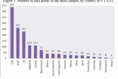
Figure 1 depicts the number of data points in the meta-sample, by country. It is

obvious that the United States provided the meta-sample with the most elasticities.

This uneven distribution of estimates over the countries came not as a surprise as the

minimum wage impact on employment has been extensively investigated in the USA

which has many states with different minimum wage systems. Moreover, in the USA

there is a federal minimum wage but there are also minimum wages across states with

variability in levels. Apart from the 28.73% of the observations which concern the

USA, another high percentage came from studies for Brazil which yielded 17.16% of

the total observations. Another country with many observations is the United

Kingdom with 231 observations (15.19%) and other countries with many elasticities

are Indonesia, Canada and New Zealand with 113, 111 and 72 elasticities,

[image:10.595.106.491.410.670.2]

respectively, while the rest of them provided less than 50.

Figure 1. Number of data points in the meta-sample, by country (n = 1.521).

Discussing on the publication bias of the elasticities in the meta-sample,

according to Sutton et al. (2000), the simplest and most commonly used method to

(11)

graph is a scatter diagram of all empirical estimates of a given phenomenon and these

estimates’ precisions (i.e. the inverse of the estimates’ standard errors, 1/SE).

However, the real problem of publication selection does not lie in the results

themselves and in the existence of publication biasness but the importance is in fact

that the large biases can impart upon any summary of empirical knowledge if we do

not correct it. Therefore, it is essential to investigate if the elasticities of the

meta-sample are characterized by publication selection biasness.

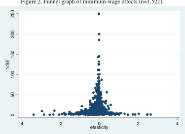
In figure 2 we present the funnel graph of the estimated minimum wage

elasticities. Clearly the graph looks symmetric, but it reflects publication selection.

Most values are gathered in the left portion of the graph which reveals selection for

negative employment effects of minimum wages. It should be noticed, though, that

these graphs are considered to be quite vulnerable to misjudgments and subjective

interpretation and criticism, so in order to test the hypothesis of presence of

publication biasness, we have to use the FAT-PET test presented in the following

section.

Closing this preliminary analysis, the general picture is that the majority of the

studies indicate a negative impact of minimum wages on employment measures. More

specifically, from the total 1.521 estimated elasticities: 944 are negative (62.06%),

564 are positive (37.08%) and 13 are equal to zero (0.85%). This means that the

impact of the neoclassical theory in the new minimum wage research is still quite

strong. However, this is only descriptive statistics analysis and in order to reach at

more reliable conclusions we conduct meta-regression analysis techniques in the next

two sections to find if there is publication bias and which factors affect the sign of the

(12)

[image:12.595.110.486.76.348.2]

Figure 2. Funnel graph of minimum-wage effects (n=1.521).

0

5

0

1

0

1

5

0

2

0

2

5

0

1

/S

E

-4 -2 0 2 4

elasticity

Note: We excluded one observation with values: elasticity = -6.07 and 1/SE = 0.433.

4. Publication bias and FAT-PET tests

The tests that appear at the title of this section are nothing more than two tests

of publication bias and authentic effect, respectively. The FAT test is a Funnel

Asymmetry Test and estimates equation (1) with the assumption that all the β1 are

zero, meaning that there is no heterogeneity. In other words, it is t-test of β0. On the

other hand, the PET test is a Precision Effect Test of β1and it tests the genuine or

authentic effect, beyond publication bias.

ti= β0+ β1(1/SEi) + vi (1)

Where,tis the t-statistic of the elasticity of theistudy,SEis the standard error

of the elasticity, andvis the error term.

Now, in order to identify if there is publication bias in the meta-sample we

follow Stanley et al. (2008) and Efendic et al. (2011) and we estimate equation (1).

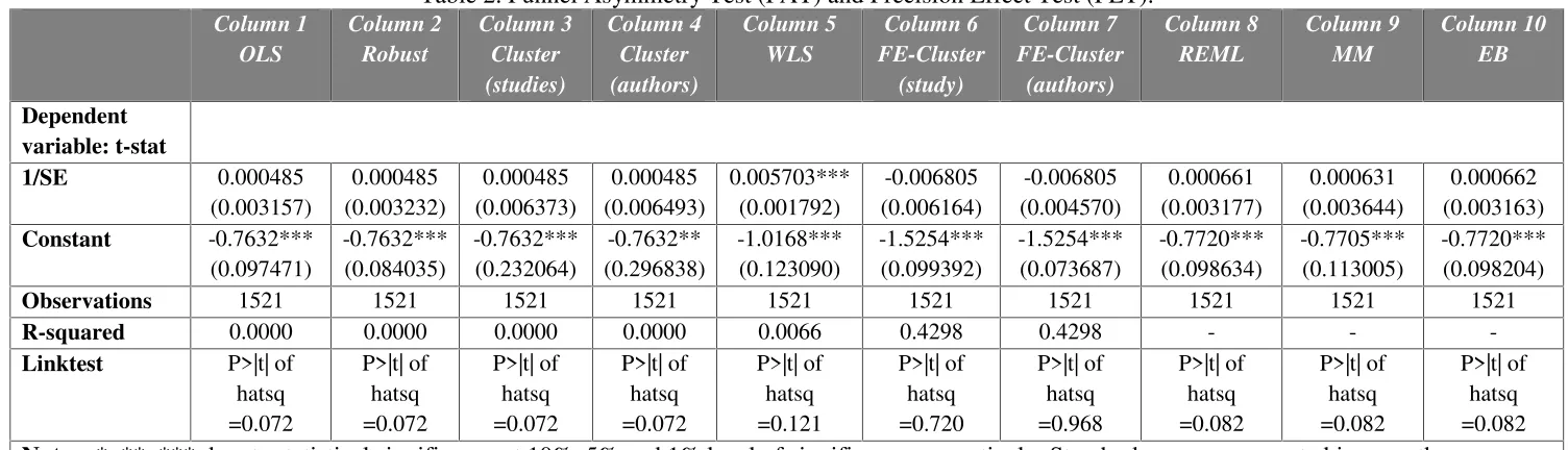
The results are presented in table 2 and indicate presence of publication bias as the

(13)

for all the estimation methods that we used which clearly implies publication selection

for negative employment effects of minimum wages.

As far as the precision of the estimated empirical effect (i.e. 1/SE) is

concerned, we performed the PET test which shows in nine out of ten estimation

methods that there is no statistically significant effect of minimum wages on

employment measures. Furthermore, the coefficients in all specifications are

extremely small which is a sign that there are no adverse employment effects of

minimum wage, results that are in agreement with the results of Doucouliagos and

Stanley’s study in (2009).

However, like any regression model, the estimates of FAT-PET tests can

become biased when important explanatory variables are omitted. Clearly, a model

cannot be explained by a single independent variable, therefore the previous model in

equation (1) should be expanded to include moderator variables that explain variation

in elasticities. For this reason the results of the FAT-PET tests should be treated with

caution and without making strong and definite conclusions. In the following section

we add into the model 27 possible moderators that take into account the study

(14)

[image:14.842.44.796.82.298.2]

Table 2. Funnel Asymmetry Test (FAT) and Precision Effect Test (PET). Column 1 OLS Column 2 Robust Column 3 Cluster (studies) Column 4 Cluster (authors) Column 5 WLS Column 6 FE-Cluster (study) Column 7 FE-Cluster (authors) Column 8 REML Column 9 MM Column 10 EB Dependent variable: t-stat 1/SE 0.000485 (0.003157) 0.000485 (0.003232) 0.000485 (0.006373) 0.000485 (0.006493) 0.005703*** (0.001792) -0.006805 (0.006164) -0.006805 (0.004570) 0.000661 (0.003177) 0.000631 (0.003644) 0.000662 (0.003163) Constant -0.7632*** (0.097471) -0.7632*** (0.084035) -0.7632*** (0.232064) -0.7632** (0.296838) -1.0168*** (0.123090) -1.5254*** (0.099392) -1.5254*** (0.073687) -0.7720*** (0.098634) -0.7705*** (0.113005) -0.7720*** (0.098204)

Observations 1521 1521 1521 1521 1521 1521 1521 1521 1521 1521

R-squared 0.0000 0.0000 0.0000 0.0000 0.0066 0.4298 0.4298 - -

-Linktest P>|t| of hatsq =0.072 P>|t| of hatsq =0.072 P>|t| of hatsq =0.072 P>|t| of hatsq =0.072 P>|t| of hatsq =0.121 P>|t| of hatsq =0.720 P>|t| of hatsq =0.968 P>|t| of hatsq =0.082 P>|t| of hatsq =0.082 P>|t| of hatsq =0.082

Notes:*, **, *** denote statistical significance at 10%, 5% and 1% level of significance respectively. Standard errors are reported in parentheses. Column 1 presents the results using the ordinary-least-squares estimation method.

Column 2 reports the robust regression version of the OLS estimation.

Column 3 presents clustered data analysis to account for within-study dependence with cluster-robust standard errors in parentheses (79 clusters).

Column 4 presents clustered data analysis to account for within-author dependence with cluster-robust standard errors in parentheses. This method is using author identiﬁers to allow for dependence within a given author’s, or group of authors’, reported elasticities. (64 clusters).

Column 5 presents the results using the weighted-least-squares estimation method.

Columns 6 and 7 present the results of columns 3 and 4, respectively using fixed (study) effects. Column 8 presents the results with restricted maximum likelihood (REML).

Column 9 presents the results with the moment estimator (MM).

Column 10 presents the results with the empirical Bayes iterative procedure (EB).

(15)

5. Meta Regression Analysis (MRA) and results

The Funnel Asymmetry Test (FAT) and the Precision Effect Test (PET)

performed in the previous section suggested evidence of publication selection and no

genuine effect of minimum wages on employment measures, respectively. However,

these tests do not take into account the heterogeneity across the studies which arises

from the fact that the expected value of a reported estimate will often depend on many

other factors like the estimation method, measurement of the dependent variable,

presence of additional controllers in the specification, business circle indicators,

structure of the data, country or a region, a group or the total population. If the

researcher does not tackle the problem of heterogeneity, bias can arise in any

meta-regression analysis estimation. However, identification of the potential variables that

can explain heterogeneity across the results is a difficult and cost-timing task.

In our analysis, we try to take into account as many as possible sources of

heterogeneity and we identified 27 moderators as potential explanatory variables of

the heterogeneity across the elasticities of the studies. These moderators which

diversified the degree of the employment effect of minimum wages, concern mainly

the study characteristics related to the data, the model specifications and the group of

(16)

[image:16.595.23.580.86.740.2]

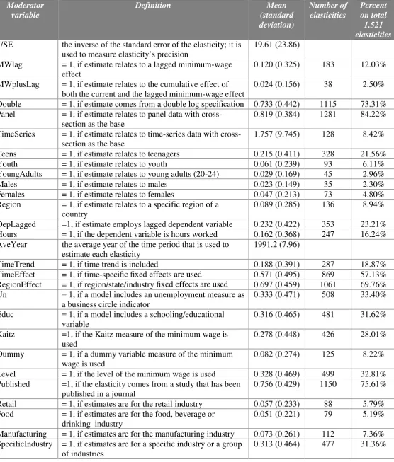
Table 3. Moderator variables for meta-regression analysis. Moderator variable Definition Mean (standard deviation) Number of elasticities Percent on total 1.521 elasticities 1/SE the inverse of the standard error of the elasticity; it is

used to measure elasticity’s precision

19.61 (23.86)

MWlag = 1, if estimate relates to a lagged minimum-wage effect

0.120 (0.325) 183 12.03%

MWplusLag = 1, if estimate relates to the cumulative effect of both the current and the lagged minimum-wage effect

0.024 (0.156) 38 2.50%

Double = 1, if estimate comes from a double log speciﬁcation 0.733 (0.442) 1115 73.31% Panel = 1, if estimate relates to panel data with

cross-section as the base

0.819 (0.384) 1281 84.22%

TimeSeries = 1, if estimate relates to time-series data with cross-section as the base

1.757 (9.745) 128 8.42%

Teens = 1, if estimate relates to teenagers 0.215 (0.411) 328 21.56%

Youth = 1, if estimate relates to youth 0.061 (0.239) 93 6.11%

YoungAdults = 1, if estimate relates to young adults (20-24) 0.029 (0.169) 45 2.96%

Males = 1, if estimate relates to males 0.023 (0.149) 35 2.30%

Females = 1, if estimate relates to females 0.047 (0.213) 73 4.80% Region = 1, if estimate relates to a specific region of a

country

0.089 (0.285) 136 8.94%

DepLagged =1, if estimate employs lagged dependent variable 0.232 (0.422) 353 23.21% Hours = 1, if the dependent variable is hours worked 0.162 (0.368) 247 16.24% AveYear the average year of the time period that is used to

estimate each elasticity

1991.2 (7.96)

TimeTrend = 1, if time trend is included 0.188 (0.391) 287 18.87% TimeEffect = 1, if time-specific fixed effects are used 0.571 (0.495) 869 57.13% RegionEffect = 1, if region/state/industry fixed effects are used 0.697 (0.459) 1061 69.76% Un = 1, if a model includes an unemployment measure as

a business circle indicator

0.333 (0.471) 508 33.40%

Educ = 1, if a model includes a schooling/educational variable

0.316 (0.465) 481 31.62%

Kaitz =1, if the Kaitz measure of the minimum wage is used

0.278 (0.448) 426 28.01%

Dummy = 1, if a dummy variable measure of the minimum wage is used

0.082 (0.274) 125 8.22%

Level = 1, if the level of the minimum wage is used 0.328 (0.469) 499 32.81% Published =1, if the elasticity comes from a study that has been

published in a journal

0.756 (0.429) 1150 75.61%

Retail = 1, if estimates are for the retail industry 0.057 (0.233) 88 5.79% Food = 1, if estimates are for the food, beverage or

drinking industry

0.051 (0.221) 79 5.19%

Manufacturing = 1, if estimates are for the manufacturing industry 0.073 (0.261) 112 7.36% SpecificIndustry = 1, if estimates are for a specific industry or a group

of industries

(17)

Commenting on the structure of the data, it is obvious that the vast majority of

the elasticities has been drawn from paneldatasets (84.22%), while only the 8.42% of

the observations were derived fromtime-seriesdata which were largely used until the

early 90’s but since then they have been relatively abandoned in the minimum wage

research. The rest 7.36% of the elasticities of the meta-sample came from

cross-section datasets. The estimations that came from minimum wage variables which

were in laggedform were 183 from the total 1.521 and the cases where the estimates

related to the total effect of both the current and the lagged minimum-wage effect

were only 38. Generally, the lagged form of the minimum wage variable is considered

to provide a long-term impact which triggered some researchers to investigate the

effect of minimum wages not only in the short-term, but also in the long-run.

The 73.31% of the elasticities of the meta-sample came from a double log

speciﬁcation while the rest 26.69% came either from single log specification

(semi-elasticities measure the percentage change in the dependent variable when the

dependent one changes by one unit) or the classic elasticity definition calculating

ni=αi./.We also included moderators relating to the age group of the population

sample providing 328 observations relating only to teenagers, 93 observations

relating to youth, and 45 elasticities relating to young adults aged 20-24 years-old.

Sub-group demographic estimates relating to elasticities to only males or females

provided only 35 and 73 observations in the meta-sample, respectively.

The explanatory variable region was included to control for any differences

between region-specific and whole country elasticities, and according the data only

8.94% of the elasticities related to a specific region of a country. The variable

(18)

353 observations of the total 1.521 came from specifications that used a lagged

dependent variable as a dependent one, i.e. almost one to four.

In the literature, as Doucouliagos and Stanley (2009) at p. 418 refer, there is

some debate about the need to control for cyclical effects and school enrolment.

Therefore, we included the variablesUn andEducto catch these effects. As indicated

in table 3, 508 observations came from a model that included an unemployment

measure as a business circle indicator, and 481 observations came from models which

included a schooling or educational variable. Furthermore, 83.76% of the elasticities

where taken form specifications that used an employment measure as dependent

variable, but 16.24% used as dependent variable thehoursworked.

Characteristics related to the sample period of the estimation where also taken

into account and we included the average year (AveYear) of the time period that was

used in each study, or to be more precise in each specification in the studies. The

effects of the use of fixed effects and time-trend in the studies were explored through

TimeTrend, TimeEffect and RegionEffect variables. A large group of estimates came

from studies that used cross-section fixed effects as 1.061 elasticities were taken from

studies which used region, state, or industry fixed effects in the specification of the

estimated model. In addition to this, large is also the group of elasticities taken from

studies which used time specific fixed effects (mostly year-fixed effects) providing

869 elasticities. Lastly, 287 elasticities were taken from studies which included a time

trend.

Across the studies we found a great variability of the minimum wage measure

that was used to investigate the impact on employment. We tried to categorize the

potential minimum wage measurements into the following groups: 32.81% of the

(19)

minimum wage (minimum/average wage), while 8.22% used a dummy variable

measurement of the minimum wage. The rest 30.96% used other minimum wage

measures such as proportion at or below minimum wage, minimum wage*crisis

dummy and others.

The majority of the elasticities of the meta-sample came from studies that have

been published in an academic journal (75.61%). However, there are elasticities that

come from unpublished studies which are mainly working papers cited in article

papers and books, and some of them will be published in a journal. Therefore, we

found it appropriate to include them into the meta-sample.

Closing our analysis on the moderators, we would say that the all-set

meta-sample includes elasticities for specific industries of a country; therefore we should

include controls to investigate any such differences. We used three moderatorsRetail,

Food, and Manufacturing which provided the most elasticities in comparison to the

other industries, and an addition one SpecificIndustry if estimates are generally for a

specific industry or a group of industries. Numerically, 88 elasticities are for the retail

industry, 79 are for the food, beverage or drinking industry, 112 are for the

manufacturing industry, and totally 477 elasticities are related to the employment

effect of minimum wages in a single industry or a group of industries but not the

whole economy.

Now, taking into account the study heterogeneity, we follow Adam et. al.

(2013) and we incorporate the moderator variables as potential explanatory variables

of this heterogeneity. Then, the meta-regression model we estimate takes the form:

ti=β0+β1(1/SEi) +





K

k j jk k

SE Z a

1

(20)

Where,tis the t-statistic of the elasticity of theistudy,SEis the standard error

of the elasticity of the i study, Zk are the K moderator variables, and vj is the error

term.

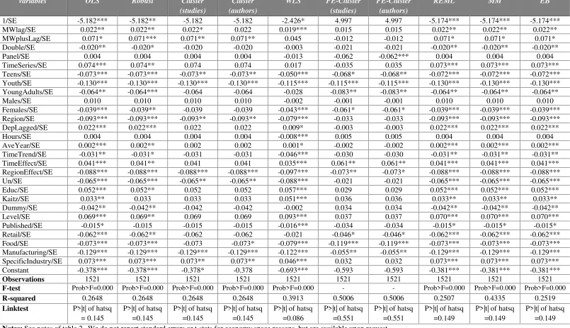
Table 4 presents the results of the meta-regression analysis using all the

moderators in the model estimations. In order to improve further the robustness of the

results, we applied 10 estimation methods which generally did not cause variability in

the estimated coefficients. In column 1, we present the results using the

ordinary-least-squares estimation method which indicates that effects that relate to teenagers,

youth and young adults tend to report a negative and statistically significant impact of

minimum wage on employment measures. The same appears for elasticities related to

females, and for a specific region of the country. In addition, specifications that

employ a timetrend or fixed region effects, that use unemployment as controller, if

minimum wage is a dummy variable, or in case the study is published, then they

report a negative relationship between minimum wages and employment. Those

elasticities which are related to retail sector, food, beverage or drinking industry or

manufacturing, report negative minimum wage effects.

On the other hand, elasticities from minimum wage variables in lagged form,

or if they report the cumulative effect of both current and lagged minimum wage, they

both indicate positive effect of minimum wages on employment. Moreover, studies

with time-series data, elasticities from dynamic specifications, specifications with

time fixed effects, or if they employ an educational variable, they seem to report

positive employment effects of minimum wages. Furthermore, kaitz index measures

or the minimum wage level report positive impact and the same happens when

generally the elasticity comes from a specific industry or a group of industries. The

(21)

with time the effect of minimum wages tends to provide positive estimations. Finally,

panel, males and hours variables do not appear to explain any heterogeneity of the

minimum wage elasticities.

In column 2 we present the robust regression version of the OLS estimation

which provides almost the same results with slight differences. In column 3 clustered

data analysis is reported to account for within-study dependence with cluster-robust

standard errors in parentheses. In the literature of meta-analysis, it is a usual

phenomenon to be reported estimation results with clusters across the studies.

However, having so many studies in the meta-sample may mean that some of them

have the same author or authors, fact which causes biasness of the results. Therefore,

we implemented cluster data analysis in column 4 using author identiﬁers to allow for

dependence within a given author’s, or group of authors’, reported elasticities. The

analysis showed that the 79 studies of the meta-sample were written by 64 author(s),

therefore we also used clustered data analysis to account for within-author

dependence. Results in columns 3 and 4 do not change in sign and magnitude but the

moderators: TimeSeries, YoungAdults, Females, DepLagged, AveYear, TimeTrend,

TimeEffect, Educ, Dummy, Level, Retail and Kaitz (divided by SE) are no longer

statistically significant.

Column 5 presents the results using the weighted-least-squares estimation

method used first time in the meta-analysis literature of minimum wages in Stanley

and Doucouliagos (2012). Estimation results do not alter in sign but there are changes

in the magnitudes to both directions. Nevertheless, in this estimation method the

linktest accepts the null only at the 5% and 1% levels of statistical significance.

(22)

recommended. Fixed effects models assume that there is one true and common effect

that all studies are estimating and that all the variability and differences between

effect sizes is due to sampling error. This means that they essentially assume

homogeneity. This would have seen reasonable if the studies were the almost same

and identical and had same measures and same features. In this case the differences

would arise from the errors in the samples. Despite that, Stanley and Doucouliagos in

their book in 2012 imply that fixed effects are more suitable in economics

meta-analysis but not in psychology and medicine and use fixed effects specification in

their book extensively. Now, in the clustered data analysis with fixed effect presented

in columns 6 and 7 many moderators lost their indicator of statistical significance but

they do not change in sign and some of them remain statistical significant.

In columns 8, 9 and 10 we apply random effects models. Random effects

assume that there are multiple effects which the studies are estimating and that

variability between effect sizes is due to sampling error plus some variability from

true study differences. There are genuine differences among studies so random effects

models, generally, are preferred in meta-analysis to take into account this variability.

Column 8 shows the results with Restricted Maximum Likelihood (REML) and

column 9 presents the results with the moment estimator (MM) which is the only non

iterative method which is fast and robust, but according to Mavridis and Salanti

(2012) the Maximum Likelihood methods are often preferred to MM methods as the

former have higher probability of being close to the quantities to be estimated.

Column 10 presents the results with the empirical Bayes iterative procedure (EB). All

these three random effects methods provided very similar results with the OLS

estimation with only minor and rare differences, which happens when moderate or

(23)

Commenting on the reliability of the models presented in table 4, we

performed linktests which accepted the null hypothesis at all levels of statistical

significance in nine of the ten methods, and at the 5% and 1% levels of statistical

significance in one, indicating a correct specification of the dependent variable.

Towards the same direction are the results of the F-test which is zero in all cases, and

the values of R-squared being over 25% in columns are considered to be more than

satisfactory for meta-analysis. At this point we have to point out that in columns 8-10

only the adjusted R-squared are provided from the program STATA and therefore we

report them as being R-squared. As a final comment on table 4 we would say that the

coefficient of 1/SE which indicates the minimum wage effect, in six columns it is

negative and statistically significant, implying a negative relationship. When cluster

data analysis is used in columns 3 and 4 it is no longer significant and when fixed

effects are employed in the clustered data analysis in columns 6 and 7, the coefficients

(24)

[image:24.842.20.825.41.504.2]

Table 4. Multivariate, Meta-regression analysis using all moderators (Dependent variable: t-statistic). Moderator variables Column 1 OLS Column 2 Robust Column 3 Cluster (studies) Column 4 Cluster (authors) Column 5 WLS Column 6 FE-Cluster (studies) Column 7 FE-Cluster (authors) Column 8 REML Column 9 MM Column 10 EB

1/SE -5.182*** -5.182** -5.182 -5.182 -2.426* 4.997 4.997 -5.174*** -5.174*** -5.174***

MWlag/SE 0.022** 0.022** 0.022* 0.022 0.019*** 0.015 0.015 0.022** 0.022** 0.022**

MWplusLag/SE 0.071* 0.071*** 0.071** 0.071** 0.045 -0.012 -0.012 0.071* 0.071* 0.071*

Double/SE -0.020** -0.020* -0.020 -0.020 -0.003 -0.021 -0.021 -0.020** -0.020** -0.020**

Panel/SE 0.004 0.004 0.004 0.004 -0.013 -0.062 -0.062*** 0.004 0.004 0.004

TimeSeries/SE 0.074*** 0.074** 0.074 0.074 0.017 -0.035 0.035 0.073*** 0.073*** 0.073***

Teens/SE -0.073*** -0.073*** -0.073** -0.073** -0.050*** -0.068* -0.068** -0.072*** -0.072*** -0.072***

Youth/SE -0.130*** -0.130*** -0.130*** -0.130*** -0.115*** -0.115*** -0.115*** -0.130*** -0.130*** -0.130***

YoungAdults/SE -0.064** -0.064*** -0.064 -0.064 -0.028 -0.083** -0.083** -0.064** -0.064** -0.064**

Males/SE 0.010 0.010 0.010 0.010 -0.002 -0.001 -0.001 0.010 0.010 0.010

Females/SE -0.039*** -0.039** -0.039 -0.039 -0.043*** -0.061* -0.061* -0.039*** -0.039*** -0.039***

Region/SE -0.093*** -0.093*** -0.093** -0.093** -0.079*** -0.033 -0.033 -0.093*** -0.093*** -0.093***

DepLagged/SE 0.022*** 0.022*** 0.022 0.022 0.009* -0.003 -0.003 0.022*** 0.022*** 0.022***

Hours/SE 0.004 0.004 0.004 0.004 -0.008*** 0.005 0.005 0.004 0.004 0.004

AveYear/SE 0.002*** 0.002** 0.002 0.002 0.001* -0.002 -0.002 0.002*** 0.002*** 0.002***

TimeTrend/SE -0.031** -0.031* -0.031 -0.031 -0.046*** -0.030 -0.030 -0.031** -0.031** -0.031**

TimeEffect/SE 0.041*** 0.041** 0.041 0.041 0.035*** 0.061** 0.061** 0.041*** 0.041*** 0.041***

RegionEffect/SE -0.088*** -0.088*** -0.088*** -0.088*** -0.097*** -0.073** -0.073* -0.088*** -0.088*** -0.088***

Un/SE -0.065*** -0.065*** -0.065** -0.065** -0.088*** -0.021 -0.021 -0.065*** -0.065*** -0.065***

Educ/SE 0.052*** 0.052** 0.052 0.052 0.057*** 0.029 0.029 0.052*** 0.052*** 0.052***

Kaitz/SE 0.033** 0.033 0.033 0.033 0.051*** 0.036 0.036 0.033** 0.033** 0.033**

Dummy/SE -0.042** -0.042** -0.042 -0.042 -0.002 0.034 0.034 -0.042** -0.042** -0.042**

Level/SE 0.069*** 0.069** 0.069 0.069 0.093*** 0.037 0.037 0.070*** 0.070*** 0.070***

Published/SE -0.015* -0.015 -0.015 -0.015 -0.016*** -0.034 -0.034 -0.015* -0.015* -0.015*

Retail/SE -0.062*** -0.062** -0.062 -0.062 -0.021 -0.046* -0.046* -0.062*** -0.062*** -0.062***

Food/SE -0.073*** -0.073*** -0.073 -0.073* -0.079*** -0.119*** -0.119*** -0.073*** -0.073*** -0.073***

Manufacturing/SE -0.129*** -0.129*** -0.129*** -0.129*** -0.122*** -0.055** -0.055** -0.129*** -0.129*** -0.129***

SpecificIndustry/SE 0.073*** 0.073*** 0.073** 0.073** 0.046*** 0.032 0.032 0.073*** 0.073*** 0.073***

Constant -0.378*** -0.378*** -0.378* -0.378 -0.693*** -0.593 -0.593 -0.381*** -0.381*** -0.381***

Observations 1521 1521 1521 1521 1521 1521 1521 1521 1521 1521

F-test Prob>F=0.000 Prob>F=0.000 Prob>F=0.000 Prob>F=0.000 Prob>F=0.000 - - Prob>F=0.000 Prob>F=0.000 Prob>F=0.000

R-squared 0.2648 0.2648 0.2648 0.2648 0.3913 0.5006 0.5006 0.2507 0.4335 0.2519

Linktest P>|t| of hatsq = 0.145

P>|t| of hatsq =0.145

Notes:See notes of table 2. We do not report standard errors or t-stats for economy space reasons, but are available upon request.

(25)

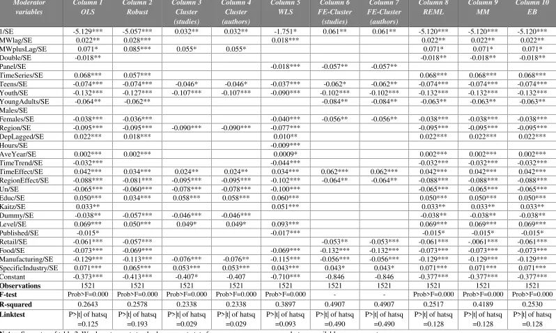
In table 5 we apply the General-to-Specific approach following Stanley and

Doucouliagos (2012) and Benos and Zotou (2014). This method begins having all the

explanatory variables in the equation that we want to estimate. Afterwards, we

removed the least statistically significant, one at time, until all variables which

remained to be statistically significant. It may not seem ideal but as Charemza and

Deadman (1997) refer at page 78 of their book: ‘the strength of general to specific

modeling is that the model construction proceeds from a very general model in a more

structured, ordered fashion, and in this way avoids the worst of data missing’.

Additionally, as Stanley and Doucouliagos (2012) state at page 91 in their book: ‘the

other sensible approach is to report only the MRA model that includes all coded

moderator variables’, which is what we did in table 4.

Generally, the results in table 5 are similar to those of table 4. Ten moderators

(MWlag, MWplusLag, TimeSeries, DepLagged, AveYear, TimeEffect, Educ, Kaitz,

Level and SpecificIndustry, divided by SE) have positive coefficients and fifteen

moderators (Double, Panel, Teens, Youth, YoungAdults, Females, Region,

TimeTrend, RegionEffect, Un, Dummy, Published, Retail, Food and Manufacturing,

divided by SE) report negative coefficients. Moderator related to Hours has a small

but statistically significant negative coefficient in only the WLS column, and

moderator related to Males does not provide a statistical significant estimation in any

(26)

[image:26.842.25.823.25.503.2]

Table 5. Multivariate, General-to-Specific, Meta-regression analysis (Dependent variable: t-statistic). Moderator variables Column 1 OLS Column 2 Robust Column 3 Cluster (studies) Column 4 Cluster (authors) Column 5 WLS Column 6 FE-Cluster (studies) Column 7 FE-Cluster (authors) Column 8 REML Column 9 MM Column 10 EB

1/SE -5.129*** -5.057*** 0.032** 0.032** -1.751* 0.061** 0.061** -5.120*** -5.120*** -5.120***

MWlag/SE 0.022** 0.028*** 0.018*** 0.022** 0.022** 0.022**

MWplusLag/SE 0.071* 0.085*** 0.055* 0.055* 0.071* 0.071* 0.071*

Double/SE -0.018** -0.018** -0.018** -0.018**

Panel/SE -0.018*** -0.057** -0.057**

TimeSeries/SE 0.068*** 0.057*** 0.068*** 0.068*** 0.068***

Teens/SE -0.074*** -0.074*** -0.046* -0.046* -0.037*** -0.062* -0.062** -0.074*** -0.074*** -0.074***

Youth/SE -0.132*** -0.127*** -0.107*** -0.107*** -0.090*** -0.102*** -0.102*** -0.132*** -0.132*** -0.132***

YoungAdults/SE -0.064** -0.062** -0.084** -0.084** -0.063** -0.063** -0.063**

Males/SE

Females/SE -0.038*** -0.036*** -0.040*** -0.056** -0.056** -0.038*** -0.038*** -0.038***

Region/SE -0.095*** -0.095*** -0.090*** -0.090*** -0.077*** -0.095*** -0.095*** -0.095***

DepLagged/SE 0.022*** 0.018*** 0.010** 0.022*** 0.022*** 0.022***

Hours/SE -0.009***

AveYear/SE 0.002*** 0.002*** 0.0009* 0.002*** 0.002*** 0.002***

TimeTrend/SE -0.032*** -0.044*** -0.032*** -0.032*** -0.032***

TimeEffect/SE 0.042*** 0.034*** 0.024** 0.024** 0.034*** 0.062*** 0.062*** 0.042*** 0.042*** 0.042***

RegionEffect/SE -0.088*** -0.081*** -0.095*** -0.095*** -0.102*** -0.064** -0.064** -0.088*** -0.088*** -0.088***

Un/SE -0.065*** -0.060*** -0.078*** -0.078*** -0.100*** -0.065*** -0.065*** -0.065***

Educ/SE 0.050*** 0.034*** 0.058*** 0.058*** 0.060*** 0.050*** 0.050*** 0.050***

Kaitz/SE 0.033** 0.051*** 0.033** 0.033** 0.033**

Dummy/SE -0.038** -0.057*** -0.046*** -0.046*** -0.038** -0.038** -0.038**

Level/SE 0.069*** 0.050*** 0.049* 0.049* 0.093*** 0.069*** 0.069*** 0.069***

Published/SE -0.015* -0.017*** -0.015* -0.015* -0.015*

Retail/SE -0.061*** -0.057*** -0.053** -0.053*** -0.061*** -.0061*** -0.061***

Food/SE -0.073*** -0.069*** -0.069*** -0.132*** -0.132*** -0.073*** -0.073*** -0.073***

Manufacturing/SE -0.129*** -0.113*** -0.076*** -0.076** -0.115*** -0.056*** -0.056*** -0.129*** -0.129*** -0.129***

SpecificIndustry/SE 0.071*** 0.065*** 0.053*** 0.053*** 0.043*** 0.043* 0.043* 0.071*** 0.071*** 0.071***

Constant -0.373*** -0.413*** -0.407* -0.407 -0.710*** -0.846 -0.846 -0.377*** -0.377*** -0.377***

Observations 1521 1521 1521 1521 1521 1521 1521 1521 1521 1521

R-squared 0.2643 0.2578 0.2338 0.2338 0.3897 0.4907 0.4907 0.2517 0.4189 0.2530

Linktest P>|t| of hatsq =0.125

Notes:See notes of table 2. We do not report standard errors or t-stats for economy space reasons, but are available upon request.

(27)

6. Robustness checks

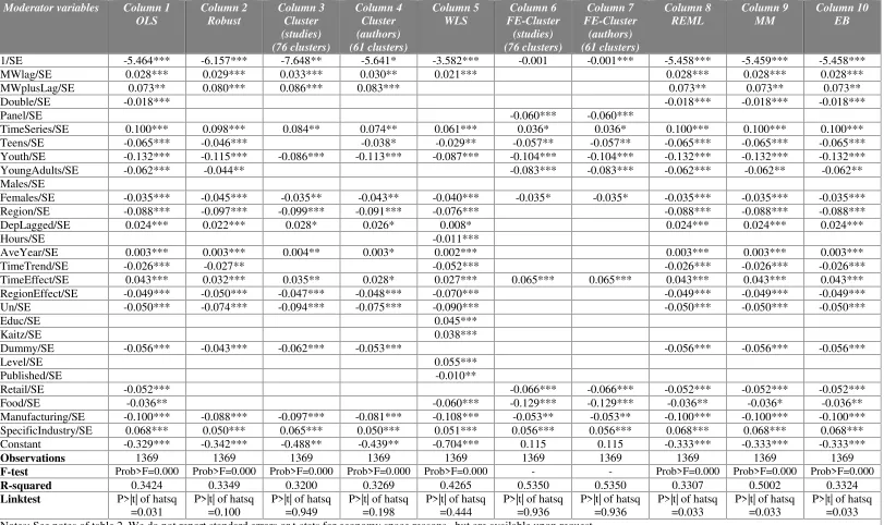
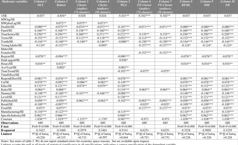
In tables 6-9, we examine the sensitivity of the previous results by conducting

four robustness checks. Initially, in table 6 we excluded the 10% of the extreme

values in the meta-sample. To be more specific, in the first robustness check we

excluded the highest 5% and the lowest 5% values of the elasticities, which reduced

the meta-sample by 152 elasticities. The general picture is not altered which is very

encouraging for the robustness of our previous results, as the signs of the moderators

did not change when we excluded the “outliers” of the meta-sample. As slight

exceptions we would mention that moderator related to RegionEffect/SE decreased in

magnitude, and that moderators related to Educ/SE, Kaitz/SE, Level/SE,

Published/SE appear to be statistically significant in only one column out of ten.

In table 7 we excluded all the statistically insignificant elasticities of the

meta-sample, which led to the reduction of the sample by 841 elasticities. We performed

the General-to-Specific methodology to the remaining 680 elasticities and our

previous results generally seemed to hold with only small differences. The only

exception is in the case of the moderator related to Panel, where there is a change in

the sign. When we keep only the statistically significant elasticities in the

meta-sample, this moderator suggests positive employment effect of minimum wage in 8

out of 10 columns. Furthermore, moderator related to Hours is now positive in 5

columns, but generally the results for the other moderators do not seem to change

greatly. However, the most remarkable result in this robustness check is that in all

columns the moderator Published has negative value, clearly implying that published

studies have a tension to report negative employment elasticities of minimum wage.

(28)

following robustness check where we exclude all the elasticities that come from

unpublished studies.

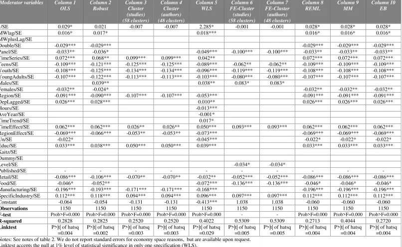
In the third robustness analysis we exclude all the elasticities that come from

an unpublished study and the results are displayed in table 8. In this robustness check

we follow Stanley and Doucouliagos (2012) who state at page 19 that: ‘If unpublished

studies have been collected, it is probably wise to undertake a sensitivity analysis of

the meta-analysis, that is, conduct the meta-analysis with and without unpublished

papers’. The unpublished studies provided 371 elasticities in our meta-sample and

after the exclusion of them, 1.150 elasticities remained. In comparison to the previous

tables, the results are relatively similar with a few exceptions. First of all moderators

MWplusLag/SE, Kaitz/SE and Dummy/SE are not statistically significant in any

estimation method. Secondly, the results for teens, youth and young adults are almost

the same in magnitude and their sign, once again, indicates that if the study focuses on

people who belong to these age groups, then the neoclassical theory, which suggests

negative employment effect of minimum wage, prevails. In case the study employees

a time trend or uses the level of the minimum wage as measurement of the minimum

wage, we can see a change in the sign compared to the previous tables. TimeTrend/SE

is positive in only one column and Level/SE is negative in only two columns, though.

We would mention that the estimation results in columns 1, 8, 9 and 10 are almost the

same, and in columns 3 and 4, and 6 and 7 they are exactly the same, respectively.

Finally, in table 9 we perform the General-to-Specific methodology by adding

two additional moderators which relate to the country. More specifically, we included

the USA/SE moderator if the elasticity comes from a study conducted for the United

States, and moderator Europe/SE if the elasticity comes from a European country,

(29)

obtained from US studies (28.7%), 377 from studies conducted for European

countries (24.8%) and 707 from studies elsewhere (46.5%). As far as these new two

moderators is concerned, it is shown that USA studies do not report a preference for

positive or negative employment effects of minimum wage, whereas, studies

conducted for European countries seem to report positive minimum wage elasticities.

Furthermore, the results of our analysis when we add USA and European moderators

do not change greatly. Moderators related to MWlag/SE, MWplusLag/SE,

AveYear/SE, TimeEffect/SE, Educ/SE, Level/SE, SpecificIndustry/SE are still

positive, implying positive effect of minimum wages, while moderators related to

Double/SE, Teens/SE, Youth/SE, YoungAdults/SE, Females/SE, Region/SE,

RegionEffect/SE, TimeTrend/SE, Un/SE, Dummy/SE, Published/SE, Retail/SE,

Food/SE, and Manufacturing/SE are still negative. Once again, as in table 5, variables

Males/SE and Hours/SE do not report a statistically significant coefficient, but now

the inclusion of the country moderators make DepLagged/SE and Kaitz/SE

moderators lose their statistically significance. Additionally, the two moderators

related to the structure of the data (i.e. Panel/SE and TimeSeries/SE) alter their signs

across the columns.

Given that the robustness checks generally fail to provide different results, this

adds extra robustness and stability to the meta-analysis that has been conducted.

However, it should be mentioned that there is still much unobserved heterogeneity

across the studies and the road in order to find a model that can locate and explain all

(30)

[image:30.842.20.831.29.511.2]

Table 6. Multivariate, General-to-Specific, Meta-regression analysis (Dependent variable: t-statistic).

Robustness check 1: The highest 5% and the lowest 5% values of the elasticities are excluded (152 elasticities dropped out, 1.369 remaining). Moderator variables Column 1

OLS Column 2 Robust Column 3 Cluster (studies) (76 clusters) Column 4 Cluster (authors) (61 clusters) Column 5 WLS Column 6 FE-Cluster (studies) (76 clusters) Column 7 FE-Cluster (authors) (61 clusters) Column 8 REML Column 9 MM Column 10 EB

1/SE -5.464*** -6.157*** -7.648** -5.641* -3.582*** -0.001 -0.001*** -5.458*** -5.459*** -5.458***

MWlag/SE 0.028*** 0.029*** 0.033*** 0.030** 0.021*** 0.028*** 0.028*** 0.028***

MWplusLag/SE 0.073** 0.080*** 0.086*** 0.083*** 0.073** 0.073** 0.073**

Double/SE -0.018*** -0.018*** -0.018*** -0.018***

Panel/SE -0.060*** -0.060***

TimeSeries/SE 0.100*** 0.098*** 0.084** 0.074** 0.061*** 0.036* 0.036* 0.100*** 0.100*** 0.100***

Teens/SE -0.065*** -0.046*** -0.038* -0.029** -0.057** -0.057** -0.065*** -0.065*** -0.065***

Youth/SE -0.132*** -0.115*** -0.086*** -0.113*** -0.087*** -0.104*** -0.104*** -0.132*** -0.132*** -0.132***

YoungAdults/SE -0.062*** -0.044** -0.083*** -0.083*** -0.062*** -0.062** -0.062**

Males/SE

Females/SE -0.035*** -0.045*** -0.035** -0.043** -0.040*** -0.035* -0.035* -0.035*** -0.035*** -0.035***

Region/SE -0.088*** -0.097*** -0.099*** -0.091*** -0.076*** -0.088*** -0.088*** -0.088***

DepLagged/SE 0.024*** 0.022*** 0.028* 0.026* 0.008* 0.024*** 0.024*** 0.024***

Hours/SE -0.011***

AveYear/SE 0.003*** 0.003*** 0.004** 0.003* 0.002*** 0.003*** 0.003*** 0.003***

TimeTrend/SE -0.026*** -0.027** -0.052*** -0.026*** -0.026*** -0.026***

TimeEffect/SE 0.043*** 0.032*** 0.035** 0.028* 0.027*** 0.065*** 0.065*** 0.043*** 0.043*** 0.043***

RegionEffect/SE -0.049*** -0.050*** -0.047*** -0.048*** -0.070*** -0.049*** -0.049*** -0.049***

Un/SE -0.050*** -0.074*** -0.094*** -0.075*** -0.090*** -0.050*** -0.050*** -0.050***

Educ/SE 0.045***

Kaitz/SE 0.038***

Dummy/SE -0.056*** -0.043*** -0.062*** -0.053*** -0.056*** -0.056*** -0.056***

Level/SE 0.055***

Published/SE -0.010**

Retail/SE -0.052*** -0.066*** -0.066*** -0.052*** -0.052*** -0.052***

Food/SE -0.036** -0.060*** -0.129*** -0.129*** -0.036** -0.036* -0.036**

Manufacturing/SE -0.100*** -0.088*** -0.097*** -0.081*** -0.108*** -0.053** -0.053** -0.100*** -0.100*** -0.100***

SpecificIndustry/SE 0.068*** 0.050*** 0.065*** 0.050*** 0.051*** 0.056*** 0.056*** 0.068*** 0.068*** 0.068***

Constant -0.329*** -0.342*** -0.488** -0.439** -0.704*** 0.115 0.115 -0.333*** -0.333*** -0.333***

Observations 1369 1369 1369 1369 1369 1369 1369 1369 1369 1369

R-squared 0.3424 0.3349 0.3200 0.3269 0.4265 0.5350 0.5350 0.3307 0.5002 0.3324

P>|t| of hatsq =0.033 Notes: See notes of table 2. We do not report standard errors or t-stats for economy space reasons, but are available upon request.

(31)

[image:31.842.17.828.31.525.2]

Robustness check 2: All the statistically insignificant elasticities of the meta-sample are excluded (841 elasticities dropped out, 680 remaining). Moderator variables Column 1

OLS

Column 2 Robust

Column 3 Cluster (studies) (72 clusters)

Column 4 Cluster (authors) (58 clusters)

Column 5 WLS

Column 6 FE-Cluster

(studies) (72 clusters)

Column 7 FE-Cluster

(authors) (58 clusters)

Column 8 REML

Column 9 MM

Column 10 EB

1/SE -0.037 -4.854* 0.028 0.024 -5.431** 0.102*** 0.102** -0.037 -0.037 -0.037

MWlag/SE

MWplusLag/SE 0.072** 0.075** 0.073**

Double/SE -0.080*** -0.075*** -0.074*** -0.073*** -0.107*** -0.071*** -0.071*** -0.080*** -0.080*** -0.080***

Panel/SE 0.160*** 0.168*** 0.158*** 0.160*** 0.128*** 0.160*** 0.160*** 0.160***

TimeSeries/SE 0.250*** 0.294*** 0.260*** 0.271*** 0.272*** 0.155** 0.155** 0.250*** 0.250*** 0.250***

Teens/SE -0.152*** -0.132*** -0.112*** -0.118*** -0.052*** -0.114*** -0.114*** -0.152*** -0.152*** -0.152***

Youth/SE -0.144*** -0.140*** -0.140** -0.146*** -0.080** -0.150*** -0.150*** -0.144*** -0.144*** -0.144***

YoungAdults/SE -0.124* -0.132*** -0.095* -0.157*** -0.157*** -0.124* -0.124* -0.124*

Males/SE

Females/SE -0.152*** -0.152***

Region/SE -0.078** -0.094*** -0.090*** -0.078** -0.078** -0.078**

DepLagged/SE 0.026*

Hours/SE 0.034** 0.032** 0.034** 0.034** 0.034**

AveYear/SE 0.002* 0.003**

TimeTrend/SE -0.103*** -0.075* -0.075*

TimeEffect/SE

RegionEffect/SE -0.081*** -0.076*** -0.056** -0.056** -0.078*** -0.081*** -0.081*** -0.081***

Un/SE -0.078*** -0.092*** -0.086** -0.083** -0.149*** -0.078*** -0.078*** -0.078***

Educ/SE 0.132*** 0.121*** 0.074** 0.079** 0.120*** 0.132*** 0.132*** 0.132***

Kaitz/SE 0.064** 0.068** 0.134*** 0.065** 0.065** 0.064*** 0.064** 0.064***

Dummy/SE -0.148*** -0.160*** -0.167*** -0.166*** -0.088*** -0.148*** -0.148*** -0.148***

Level/SE 0.121*** 0.117*** 0.126*** 0.121*** 0.121*** 0.121***

Published/SE -0.058*** -0.050** -0.062*** -0.062** -0.102*** -0.092*** -0.092*** -0.058*** -0.058*** -0.058***

Retail/SE -0.109*** -0.097*** -0.035* -0.035* -0.109*** -0.109*** -0.109***

Food/SE -0.073* -0.075** -0.137*** -0.137*** -0.073* -0.073* -0.073*

Manufacturing/SE -0.110*** -0.122*** -0.115*** -0.110*** -0.110*** -0.110***

SpecificIndustry/SE 0.062*** 0.066*** 0.040*** 0.062*** 0.062*** 0.062***

Constant -1.038*** -1.019*** -1.215** -1.170* -0.987*** -0.973 -0.973 -1.038*** -1.038*** -1.038***

Observations 680 680 680 680 680 680 680 680 680 680

(32)

[image:32.842.24.830.31.527.2]

Robustness check 3: Elasticities obtained from unpublished studies are excluded (371 elasticities dropped out, 1.150 remaining). Moderator variables Column 1

OLS Column 2 Robust Column 3 Cluster (studies) (58 clusters) Column 4 Cluster (authors) (48 clusters) Column 5 WLS Column 6 FE-Cluster (studies) (58 clusters) Column 7 FE-Cluster (authors) (48 clusters) Column 8 REML Column 9 MM Column 10 EB

1/SE 0.029* 0.021 -0.007 -0.007 2.285* -0.001 -0.001 0.028* 0.028* 0.028*

MWlag/SE 0.016* 0.017* 0.018*** 0.016* 0.016* 0.016*

MWplusLag/SE

Double/SE -0.029*** -0.029*** -0.029*** -0.029*** -0.029***

Panel/SE -0.033** -0.036* -0.049*** -0.100*** -0.100*** -0.033** -0.033** -0.033**

TimeSeries/SE 0.072*** 0.068** 0.099*** 0.099*** 0.042** 0.072*** 0.072*** 0.072***

Teens/SE -0.109*** -0.121*** -0.125*** -0.125*** -0.089*** -0.062** -0.062** -0.109*** -0.109*** -0.109***

Youth/SE -0.108*** -0.125*** -0.134*** -0.134*** -0.096*** -0.119*** -0.119*** -0.108*** -0.108*** -0.108***

YoungAdults/SE -0.107*** -0.122*** -0.113*** -0.113*** -0.103*** -0.080*** -0.080*** -0.107*** -0.107*** -0.107***

Males/SE 0.039** 0.038** 0.083* 0.083*

Females/SE -0.032** -0.024* -0.032** -0.032** -0.032**

Region/SE -0.091*** -0.090*** -0.107*** -0.107*** -0.053*** -0.091*** -0.091*** -0.091***

DepLagged/SE 0.026*** 0.028*** 0.010** 0.026*** 0.026*** 0.026***

Hours/SE -0.013***

AveYear/SE -0.001*

TimeTrend/SE 0.017*

TimeEffect/SE 0.062*** 0.062*** 0.026** 0.026** 0.050*** 0.093*** 0.093*** 0.062*** 0.062*** 0.062***

RegionEffect/SE -0.069*** -0.066*** -0.053** -0.053** -0.073*** -0.069*** -0.069*** -0.069***

Un/SE -0.022* -0.045*** -0.022* -0.022* -0.022*

Educ/SE 0.033*** 0.038*** 0.050*** 0.050*** 0.039*** 0.033*** 0.033*** 0.033***

Kaitz/SE Dummy/SE

Level/SE -0.034* -0.034*

Published/SE - - -

-Retail/SE -0.086*** -0.106*** -0.070** -0.070** -0.032** -0.052*** -0.052*** -0.086*** -0.086*** -0.086***

Food/SE -0.046* -0.052** -0.072*** -0.136*** -0.136*** -0.046* -0.046* -0.046*

Manufacturing/SE -0.196*** -0.193*** -0.171*** -0.171*** -0.168*** -0.196*** -0.196*** -0.196***

SpecificIndustry/SE 0.112*** 0.118*** 0.094*** 0.094*** 0.096*** 0.097*** 0.097*** 0.112*** 0.112*** 0.112***

Constant -0.064 -0.054 -0.131 -0.131 -0.413*** 1.038 1.038 -0.060 -0.060 -0.060

Observations 1150 1150 1150 1150 1150 1150 1150 1150 1150 1150

R-squared 0.2828 0.2825 0.2520 0.2520 0.4022 0.5309 0.5309 0.2713 0.4044 0.2720

P>|t| of hatsq =0.004 Notes: See notes of table 2. We do not report standard errors for economy space reasons, but are available upon request.