Influence of Temperature Dependence of Solubility on Kinetics for Reactive Diffusion in a Hypothetical Binary System

Influence of Temperature Dependence of Solubility on Kinetics

for Reactive Diffusion in a Hypothetical Binary System

Masanori Kajihara

Department of Materials Science and Engineering, Tokyo Institute of Technology, Yokohama 226-8502, Japan

Influence of temperature dependence of solubility for each phase on kinetics of reactive diffusion has been theoretically analyzed for a hypothetical binary system consisting of two primary solid-solution phases (and) and one compound phase (). For the analysis, we consider that thephase is produced owing to the reactive diffusion between theandphases in a semi-infinite diffusion couple and the growth of the

phase is controlled by volume diffusion. In such a case, the parabolic relationship holds good between the thicknesslof thephase and the annealing timetas follows:l2_{¼Kt. Here, the parabolic coefficientKis mathematically expressed as a function of the interdiffusion coefficients}

and the solubility ranges of the,andphases. The temperature dependencies of the parabolic coefficientK, the solubility rangey

and the interdiffusion coefficient D _{of the (¼; ; ) phase are described by Arrhenius equations of K¼K}

0expðQK=RTÞ,

y_¼y

0expðQ=RTÞandD¼D0expðQD=RTÞ, respectively. The analysis indicates thatQK is close toQ

DþQatQ

DQD and

QDQ

Dbut greater thanQ

DþQatQ

D>QDorQ

D>Q

D. As a consequence, the temperature dependency of the parabolic coefficient is directly related with those of the interdiffusion coefficient and the solubility range of the compound phase in the former case but not in the latter case. [doi:10.2320/matertrans.MRA2007316]

(Received December 10, 2007; Accepted January 21, 2008; Published March 12, 2008) Keywords: computer simulations, reactive diffusion, activation enthalpy, intermetallics

1. Introduction

Intermetallic compounds appear as stable phases in many binary alloy systems.1)When a diffusion couple is prepared from two different pure metals in such a binary system and then isothermally annealed at an appropriate temperatureT, some of the compounds may be observed as layers at the interface between the two metals after certain periods due to reactive diffusion. For various alloy systems, the kinetics of the reactive diffusion was experimentally studied by many investigators.2–33) _{When the reactive diffusion is controlled} by volume diffusion, the total thicknessl of the compound layers is mathematically expressed as a function of the annealing time tby the parabolic relationship l2_{¼Kt. The}

parabolic coefficient K is usually described as a function of the temperature T by an Arrhenius equation of K¼K0expðQK=RTÞ, where R is the gas constant. The

pre-exponential factorK0and the activation enthalpyQKcan

be evaluated by the least-squares method from experimental values of K obtained at different annealing temperatures. Most of the experimental studies indicate that the temper-ature dependence of K is reasonably expressed by the Arrhenius equation within experimental uncertainty.2–33) Thus, we may expect that the Arrhenius equation of K provides representative properties of the interdiffusion in the diffusion couple. However, complex information of the temperature dependencies of the solubility ranges and the interdiffusion coefficients of the relevant phases is included in K0 and QK. Consequently, such derivation is not so

straightforward.

The reactive diffusion controlled by volume diffusion was theoretically analyzed using a mathematical model in a previous study.34)In that analysis, a hypothetical binary alloy system composed of one intermetallic compound and two primary solid-solution phases was treated, and then the

growth rate of the compound layer was evaluated for various semi-infinite diffusion couples initially consisting of the two primary solid-solution phases. That mathematical model was also used to analyze numerically the relationship between the temperature dependence of the interdiffusion in each phase and the kinetics of the reactive diffusion.35)In the numerical analysis, the temperature dependence of the interdiffusion coefficient D was expressed by an Arrhenius equation of D¼D0expðQD=RTÞ, and the following assumptions were adopted: (a) the molar volume, the solubility range and the pre-exponential factorD0are constant and equivalent for all

the phases; and (b) the activation enthalpyQDis equivalent for the solution phases but different between the compound and the solution phase. According to the numerical analysis, the equation K¼K0expðQK=RTÞ is reliable enough to

express the temperature dependence of experimental values of K but not completely exact. If QD is smaller for the compound than for the solution phases,QKis close toQDof the compound. In this case, the temperature dependence ofK corresponds well with that of D of the compound. Such a relationship no longer holds good unlessQDis smaller for the compound than for the solution phases. In order to examine whether these conclusions are universally valid, assumption (b) was eliminated in previous numerical analyses.36,37) Nevertheless, attention was focused on the relationship between the temperature dependency of the kinetics and those of the interdiffusion coefficients of the constituent phases. As a consequence, assumption (a) still remained in these numerical analyses. Under such conditions, the validity of the relationship betweenQK andQDcould be confirmed conclusively.36,37)

Many intermetallic compounds in binary alloy systems are line compounds.1)For such a line compound, the solubility range is constant independently of the temperature. Even in such a binary system, the solubility range of the primary solid-solution phase may vary depending on the temperature. Furthermore, there are various binary alloy systems where

*_{Corresponding author, E-mail: [email protected]}

the solubility range changes depending on the temperature not only for the primary solid-solution phase but also for the intermetallic compound. In this case, the temperature dependence of the solubility range as well as that of the interdiffusion coefficient will influence the kinetics of the reactive diffusion. Hence, in a previous study,38)_{the influence} of the temperature dependence of the solubility range on the kinetics was quantitatively analyzed for the reactive diffusion in the hypothetical binary system. For the analysis, Arrhenius equations were used to express the temperature dependencies of the solubility range and the interdiffusion coefficient. However, only limited combinations of the enthalpy of solution were adopted for the intermetallic compound and the primary solid-solution phases, and thus the influence could not be confirmed conclusively. In the present study, the analysis has been extensively carried out for various combinations of the enthalpy of solution. However, there exist too many parameters determining the kinetics. Thus, for simplicity, the same temperature dependence of the inter-diffusion coefficient has been assumed for all the constituent phases. Even under such simplified conditions, valuable conclusions were drawn from the analysis.

2. Analysis

A hypothetical binary A–B system composed of one intermetallic compound and two primary solid-solution phases was considered in previous studies.34–38) The phase diagram of this binary system is represented in Fig. 1.34)In this figure, the ordinate shows the temperature T, and the abscissa indicates the mol fractionyof element B. Theand

phases are the primary solid-solution phases of elements A and B, respectively, and the phase is the compound. The same binary system was adopted in the present study. Now, we consider a semi-infinite diffusion couple consisting of the

and phases with initial compositions of y0 _{and y}0_,

respectively. The semi-infinite diffusion couple means that the thickness is semi-infinite for theand phases and the

/ interface is flat. In such a diffusion couple, the interdiffusion of elements A and B takes place unidirection-ally along the direction perpendicular to the flat interface. This direction is hereafter called the diffusional direction. When the diffusion couple is isothermally annealed atT ¼T1

for an appropriate time, the phase will be produced as a layer at the interface due to the reactive diffusion between the

andphases. If the local equilibrium is actualized at each migrating interface during annealing, the compositions of the neighboring phases at the interface coincide with those of the corresponding phase boundaries at T¼T1 in the phase

diagram of the binary A–B system indicated in Fig. 1. In this case, the migration of the interface is governed by the volume diffusion in the neighboring phases. According to the phase diagram in Fig. 1, y _{andy are the compositions of the} andphases, respectively, at the/interface, andy_and y_{are those of theand phases, respectively, at the/} interface. The compositionsy_{,y,y andyprovide the} boundary conditions, and those y0 _{and y}0 _{give the initial}

conditions.

If the reactive diffusion is controlled by the volume diffusion, the positions z _{and z of the = and =} interfaces are expressed as functions of the annealing time tby

z¼Kpffiffiffiffiffiffiffiffiffiffi4D_t¼K ffiffiffiffiffiffiffiffiffiffi

4D_t p

ð1aÞ

and

z ¼Kpffiffiffiffiffiffiffiffiffiffi4D_t¼Kpffiffiffiffiffiffiffiffiffiffi_{4Dt; ð1bÞ}

respectively.39,40) _{In eq. (1), D, D and D are the} interdiffusion coefficients for volume diffusion in the ,

and phases, respectively, andK_{,K,K andKare} dimensionless coefficients. The difference between z _and z_{is equal to the thicknesslof thelayer, and hence eq. (1)} deduces the following relationship describinglas a function oft.

l2¼ ðzzÞ2¼4DðKKÞ2t¼Kt ð2Þ

Here,Kis the parabolic coefficient defined as

K4DðKKÞ2: ð3Þ

The dimensionless coefficients are related to the initial and boundary conditions as follows:

cc¼ c 0_c

Kpffiffiffi_f1erfðKÞgexpf ðK

Þ2g

þ c

_c

Kpffiffiffi_{ferfðKÞ erfðKÞg}expfðK _Þ2_g

ð4aÞ

and

cc¼ c _c

Kpffiffiffi_{ferfðKÞ erfðKÞg}expfðK _Þ2_g

þ c

0_c

Kpffiffiffi_{f1þerfðKÞg}expfðK

Þ2g: ð4bÞ

Here,cis the concentration of element B measured in mol per unit volume. The initial and boundary conditions are indicated with the concentrationcin eq. (4), but shown with

the mol fractionyin Fig. 1. However,yis readily converted into c by the equation c¼y=Vm, where Vm is the molar volume of the relevant phase. The following relationships are obtained from eq. (1):

K¼KpffiffiffiffiffiffiffiffiffiffiffiffiffiffiD_{=D ð5aÞ}

and

K¼KpffiffiffiffiffiffiffiffiffiffiffiffiffiffiD_{=D: ð5bÞ}

According to eq. (5), only two of the four dimensionless coefficients are independent. In the present analysis,K_and K _{are chosen as the independent variables. Insertion of} eq. (5) into eq. (4) results in two independent equations. Consequently, the two independent variables are finally determined from the two independent equations. Inserting the values ofKandK into eq. (3), we obtain the parabolic coefficient K. Since K andK are functions of c0,c, c_,c,c,c0_{,D,DandDthrough eqs. (4) and (5),Kis} a function of these nine parameters.

3. Results and Discussion

As already mentioned in Section 2, the composition is indicated with the mol fraction y in Fig. 1 but with the concentration cin eq. (4). However,y is readily converted into c by the equation c¼y=Vm, where Vm is the molar volume of the relevant phase. According to the analyses in previous studies,34–38)the following assumptions have been adopted also in the present study: (A)Vm is independent of the composition; and (B)Vmis equivalent for all the phases. Due to assumptions (A) and (B),c0,c,c,c,candc0 in eq. (4) are automatically replaced withy0,y,y,y, y_andy0_{, respectively. Furthermore, we use the}

composi-tional parameters defined as

yyy0; ð6aÞ

yyy; ð6bÞ

y y0y ð6cÞ

and

y0 ðyþyÞ=2: ð6dÞ

Here, y and y0 are the solubility range and the mean composition of the phase, respectively. The initial and boundary conditions are expressed with y0_{, y}0_{, y}0_{, y,}

y_{andy. The following values were used in the present} analysis:y0_¼0,y0_¼0:5andy0_{¼1. In the case ofy}0_¼

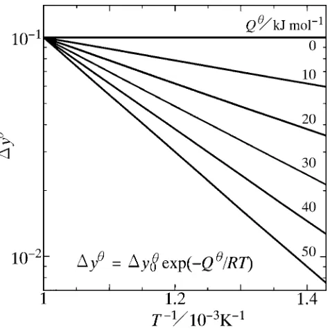
0 and y0_{¼1, y and y correspond to the solubility} ranges of the and phases, respectively. The solubility range y _{of the (¼; ; ) phase is described as a} function of the temperatureT by the following equation.

y¼y₀expðQ=RTÞ ð7Þ

Here, y₀ and Q are the pre-exponential factor and the enthalpy of solution, respectively. In the present study, Q was varied from 0 to 50 kJ/mol for the,andphases. On the other hand, y₀ was determined to yield y¼0:1 at T ¼1000K for each value ofQ. Hence,y₀¼0:1, 0.333, 1.11, 3.69, 12.3 and 40.9 are obtained forQ_{¼0, 10, 20, 30,} 40 and 50 kJ/mol, respectively. These values ofy

0 andQ

result in temperature dependencies ofy_{indicated as solid} lines in Fig. 2. In this figure, the ordinate shows the logarithm of y, and the abscissa indicates the reciprocal of T. According to the solid lines,y¼1:0101_,5:97102_,

3:57102_,2:13102_,1:27102_and7:59103_for

Q¼0, 10, 20, 30, 40 and 50 kJ/mol, respectively, at T ¼700K. As already mentioned in Section 1, the temper-ature dependence of the interdiffusion coefficientD_{for the} phase is usually expressed by

D¼D₀expðQ_D=RTÞ; ð8Þ

where D

0 and QD are the pre-exponential factor and the activation enthalpy, respectively. The parabolic coefficientK in eq. (3) is a function of y_{,y, y, D, D andD} through eqs. (3)–(5) for given values of y0_{, y}0 _{and y}0_.

Therefore, there are too many parameters determining the value ofK. In the present study, however, attention is focused on the relationship between the temperature dependency of the kinetics and those of the solubility ranges of the constituent phases. Hence, in order to simplify the analysis, values of D₀ ¼D₀¼D₀ ¼104m2/s and Q_D¼Q_D¼ Q_D¼50kJ/mol were used for the,and phases. With these parameters,Kwas numerically calculated as a function ofT from eqs. (3)–(5) atT ¼700{1000K. The temperature dependence ofKis expressed by the following equation.

K¼K0expðQK=RTÞ ð9Þ

The pre-exponential factorK0and the activation enthalpyQK

in eq. (9) were calculated in a manner similar to previous studies.35–38)

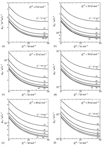
On the basis of the calculation, dependencies ofK0onQ

andQ were evaluated for various values ofQ. The results are shown as solid curves with constant values of Q ¼

0{50kJ/mol in Fig. 3. In this figure, the abscissa indicates Q, and the ordinate shows the logarithm ofK0. Figure 3(a),

(b), (c), (d), (e) and (f) indicates the results forQ¼0, 10, 20, 30, 40 and 50 kJ/mol, respectively. AtQ_{¼0kJ/mol in}

Fig. 3(a), K0 takes values around 3105m2/s. For each

solid curve, K0 monotonically decreases with increasing

value of Q_{. Since D}

0¼D

0 ¼D

0 ¼104m2/s and

Q_D¼Q_D¼Q_D¼50kJ/mol as mentioned earlier, D¼ D¼D at each temperature. Furthermore,y0¼0,y0¼

0:5 and y0¼1. Thus, the effects of Q and Q on the temperature dependence ofKare equivalent each other. As a result,K0monotonically decreases also with increasing value

of Q at a constant value of Q. On the other hand, at

Q_{¼10kJ/mol in Fig. 3(b), K}

0 takes values around

1104_m2_{/s. Also in this case, however,K}

0monotonically

decreases with increasing value ofQ _{orQ. Such} depend-encies of K0 on Q and Q are realized also at Q¼

20{50kJ/mol in Fig. 3(c)–(f). However, K0 takes values

around5104_,2103_,1102 _and3102_m2_{/s at}

Q¼20, 30, 40 and 50 kJ/mol, respectively. Therefore, it is concluded thatK0 is a monotonically decreasing function of

QandQ but a monotonically increasing function ofQ.

Fig. 3 Dependencies ofK0 onQ and Q for (a) Q¼0kJ/mol, (b)Q¼10kJ/mol, (c) Q¼20kJ/mol, (d) Q¼30kJ/mol,

(e)Q

¼40kJ/mol and (f)Q

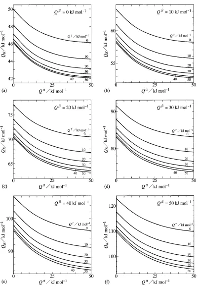
The evaluation of Fig. 3 simultaneously deduces depend-encies of QK on Q _{and Q for various values of Q. The} results are shown as solid curves with constant values of Q ¼0{50kJ/mol in Fig. 4. In this figure, the ordinate and the abscissa indicateQKandQ, respectively. The results for Q¼0, 10, 20, 30, 40 and 50 kJ/mol are shown in Fig. 4(a), (b), (c), (d), (e) and (f), respectively. As can be seen,QK as well asK0is a monotonically increasing function ofQbut a

monotonically decreasing function of Q _{andQ. At Q¼}

0kJ/mol in Fig. 4(a),QK is exactly equal to 50 kJ/mol for Q¼Q ¼0kJ/mol. As already mentioned in Section 1, the relationship between the temperature dependency of the kinetics and those of the interdiffusion coefficients of the constituent phases was numerically analyzed for a constant solubility range of each phase in previous studies.35–37) According to that analysis, QK completely coincides with

Q_D in the case of D₀ ¼D₀ ¼D₀ and Q_D¼Q_D¼Q_D. As long as Q_D<Q

D and Q D<Q

D, QK is close to Q D. If Q_D>Q

D or Q D>Q

D, however, QK becomes greater than Q_D. The values y

0 ¼y

0 ¼y

0 ¼0:1 and Q

_¼

Q_{¼Q ¼0kJ/mol result in y¼y¼y ¼0:1} independently of T according to eq. (7). Furthermore, D

0 ¼D

0¼D

0 ¼104m2/s and QD¼Q D¼ Q

D¼50kJ/ mol are considered in the present study. Under such conditions, QK completely coincides with Q_D.35–37) _{This is} just the case for the solid curve with Q_{¼0kJ/mol at} Q¼0kJ/mol in Fig. 4(a). However,QKgradually decreas-es with increasing value of Q or Q. This means that the temperature dependence of the solubility range violates the conclusions drawn in previous studies.35–37) AlthoughQK is smaller than Q_D at Q>0kJ/mol or Q>0kJ/mol, the difference betweenQK andQ_Dis rather small. On the other hand, atQ_{¼10kJ/mol in Fig. 4(b),Q}

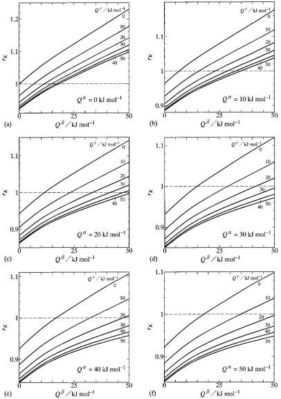
Kis greater thanQ D even atQ_{>0kJ/mol orQ >0kJ/mol, and takes values} around 60 kJ/mol. According to Fig. 4(c), (d), (e) and (f),QK is rather lose to 70, 80, 90 and 100 kJ/mol atQ_{¼20, 30, 40} and 50 kJ/mol, respectively. Compared with the dependency ofQK onQ_{, those ofQK onQandQ are less remarkable.} Therefore, it is concluded that QK is predominantly deter-mined by the summation ofQ_DandQ_{. In order to examine} the relationship between QK and the summationQ_DþQ_, the ratiorK is defined by the following equation.

rK QK=ðQþQ_DÞ ð10Þ

From eq. (10), dependencies of rK on Q and Q were estimated for various values ofQ. The results are indicated as solid curves with constant values ofQ _{¼0{50kJ/mol in} Fig. 5. In this figure, the ordinate and the abscissa show rK and Q_{, respectively. Figure 5(a), (b), (c), (d), (e) and (f)} indicates the results forQ_{¼0, 10, 20, 30, 40 and 50 kJ/mol,} respectively. As well as K0 andQK,rK is a monotonically decreasing function of Q _{and Q but a monotonically} increasing function ofQ_{. Nevertheless,rK is rather close to} unity as shown in Fig. 5. AtQ_{¼0kJ/mol in Fig. 5(a),rKis} equal to unity at Q_{¼0kJ/mol for the solid curve with} Q _{¼0kJ/mol. The valuerK ¼1is indicated as a horizontal} dashed line in Fig. 5. AsQincreases from 0 to 50 kJ/mol,rK increases from 1 to 1.23 at Q¼Q ¼0kJ/mol. On the other hand, rK decreases from 1 to 0.923 with increasing value of Q from 0 to 50 kJ/mol at Q¼Q¼0kJ/mol. Since the effects ofQandQonrK are equal to each other according to the reasons mentioned earlier,rKdecreases from 1 to 0.923 with increasing value ofQ_{from 0 to 50 kJ/mol at} Q_{¼Q ¼0kJ/mol. This clearly indicates that the} depend-ency ofrK onQis more remarkable than those ofrKonQ andQ_{. WithQ¼0kJ/mol,r}

K takes values of 0.964–1.18, 0.943–1.14, 0.931–1.12, 0.925–1.11 and 0.923–1.10 at Q_{¼0{50kJ/mol for Q ¼10, 20, 30, 40 and 50 kJ/mol,} respectively. As a result, there exist various combinations amongQ_{,QandQto realizerK¼1. Such combinations} are obtained from intersections between the solid curves and the horizontal dashed line. The intersection providesQ¼0, 6.68, 11.4, 14.7, 16.8 and 18.0 kJ/mol forQ ¼0, 10, 20, 30, 40 and 50 kJ/mol, respectively, atQ¼0kJ/mol. Owing to the equality between the effects ofQandQonrK,Q¼0, 6.68, 11.4, 14.7, 16.8 and 18.0 kJ/mol are obtained also for

Q¼0, 10, 20, 30, 40 and 50 kJ/mol, respectively, at Q _{¼0kJ/mol. According to eq. (10), the value r}

K ¼1 means QK ¼QþQ

D. In such a case, the temperature dependency of the parabolic coefficient K is directly determined from those of the solubility range y _{and the} interdiffusion coefficient D _{for the phase. In contrast, at} Q_{¼10kJ/mol in Fig. 5(b), the intersection gives} Q_{¼6:68, 15.7, 23.2, 28.7, 32.5 and 34.9 kJ/mol for} Q _{¼0, 10, 20, 30, 40 and 50 kJ/mol, respectively. At} Q_{¼20kJ/mol in Fig. 5(c), however, the intersection exists} for the solid curves withQ ¼0, 10, 20, 30 and 40 kJ/mol but not for that withQ ¼50kJ/mol withinQ¼0{50kJ/ mol. The intersection disappears for the solid curves with Q ¼30{50kJ/mol at Q¼30and 40 kJ/mol in Fig. 5(d) and (e), respectively, and for those withQ¼20{50kJ/mol atQ¼50kJ/mol in Fig. 5(f). For the solid curve without the intersection, rK is always smaller than unity. In such a case, there is no combination amongQ_{,QandQto realize} the relationshipQK¼Q

DþQ. Even in this case, however, the difference betweenQKandQ

DþQis rather small, and thus the summation Q_DþQ _{approximately represents the} temperature dependence of the parabolic coefficient K. A close relationship betweenQKandQ_DþQ_was experimen-tally observed by Taguchiet al.15)

As mentioned earlier, the relationship between the temper-ature dependency of the growth rate of the compound and those of the interdiffusion coefficients of the constituent phases was numerically analyzed for a constant solubility range of each phase in previous studies.35–37)That analysis indicates thatQKis equal toQ_DatQ_D ¼Q_D¼Q_Dand close to Q_D atQ_D<Q

D and Q D<Q

D. However, QK is greater thanQ_DatQ_D>Q

DorQ D>Q

D. Combining these relation-ships with the results in Fig. 5, we may conclude thatQK is close toQ_DþQ_atQ

DQDandQ DQ

Dbut greater than Q_DþQ _{at Q}

D>QD or Q D>Q

D. The stable crystal structure of the compound is the ordered lattice in many binary systems.1)_{In such a case,Q}

Dis greater thanQDand Q_D unless the melting temperature is much lower for the compound than for the primary solid-solution phases. For this combination ofQ

D,Q DandQ

D,QKis greater thanQ DþQ. In this case, the temperature dependency of the parabolic coefficient cannot be directly related with those of the interdiffusion coefficient and the solubility range of the compound. In order to analyze reliably the kinetics of the reactive diffusion, experimental information of the interdif-fusion coefficients and the solubility ranges of the relevant phases is essentially important.

4. Conclusions

dependencies of the interdiffusion coefficient D _{and the} solubility range y _{of the phase were described by} Arrhenius equations of D¼D₀expðQ_D=RTÞ and y¼

y₀expðQ=RTÞ, respectively. Here, D₀ andy₀ are the pre-exponential factors,Q_D is the activation enthalpy,Qis the enthalpy of solution,Ris the gas constant, andstands for

, and . For simplicity, however, the same vales of D₀¼104m2/s and Q_D¼50kJ/mol were adopted for all

the phases. On the other hand, Q _{was changed from 0 to} 50 kJ/mol, and y

0 was selected to deduce y¼0:1 at

T ¼1000K for each value ofQ. In the case of the reactive diffusion governed by volume diffusion, the square of the thickness l of the phase is proportional to the annealing time t as l2¼Kt. The temperature dependence of the parabolic coefficient K was described by an Arrhenius equation of K¼K0expðQK=RTÞ, and then the

nential factor K0 and the activation enthalpy QK were

evaluated for various combinations ofQ_{,Q andQ. Both} K0andQKare monotonically increasing functions ofQbut monotonically decreasing functions of Q _{and Q. At} Q_{¼Q¼Q ¼0kJ/mol, Q}

K is exactly equal toQ D. In such a case, representative properties of the interdiffusion in thephase may be derived from the temperature dependence of the parabolic coefficient K. As Q _{or Q increases,} however, QK becomes smaller than Q_D. In contrast, at Q_{¼10{50kJ/mol,QK is greater thanQ}

Deven at Q>0 or Q >0. Under such conditions, there exist combina-tions among Q, Q and Q to realize the relationship QK ¼QþQ_D. This relationship is reasonable approxima-tion in the wide ranges ofQ,Q andQ under the present conditions. Combining the results in previous studies35–37) with those in the present study, it is concluded that QK is close toQ_DþQ_atQ

DQ DandQ

DQ

Dbut greater than Q_DþQ _atQ

D>QDorQ D>Q

D.

Acknowledgement

The present study was supported by the Iketani Science and Technology Foundation in Japan.

REFERENCES

1) T. B. Massalski, H. Okamoto, P. R. Subramanian and L. Kacprzak: Binary Alloy Phase Diagrams, (ASM International, Materials Park, OH, 1990), vol. 1–3.

2) B. Lustman and R. F. Mehl: Trans. Met. Soc. AIME147(1942) 369– 394.

3) D. Horstmann: Stahl Eisen73(1953) 659–665.

4) S. Storchheim, J. L. Zambrow and H. H. Hausner: Trans. Met. Soc. AIME200(1954) 269–274.

5) G. V. Kidson and G. D. Miller: J. Nucl. Mater.12(1964) 61–69. 6) K. Shibata, S. Morozumi and S. Koda: J. Jpn. Inst. Met.30(1966) 382–

388.

7) K. Hirano and Y. Ipposhi: J. Jpn. Inst. Met.32(1968) 815–821. 8) M. M. P. Janssen: Metall. Trans.4(1973) 1623–1633.

9) G. F. Bastin and G. D. Rieck: Metall. Trans.5(1974) 1817–1826. 10) M. Onishi and H. Fujibuchi: Trans. JIM16(1975) 539–547. 11) EI-B. Hannech and C. R. Hall: Mater. Sci. Tech.8(1992) 817–824.

12) P. T. Vianco, P. F. Hlava and A. L. Kilgo: J. Electron. Mater.23(1994) 583–594.

13) M. Watanabe, Z. Horita and M. Nemoto: Interface Science4(1997) 229–241.

14) S. Choi, T. R. Bieler, J. P. Lucas and K. N. Subramanian: J. Electron. Mater.28(1999) 1209–1215.

15) O. Taguchi, G. P. Tiwari and Y. Iijima: Mater. Trans.44(2003) 83–88. 16) T. Yamada, K. Miura, M. Kajihara, N. Kurokawa and K. Sakamoto:

Mater. Sci. Eng. A390(2005) 118–126.

17) T. Takenaka, S. Kano, M. Kajihara, N. Kurokawa and K. Sakamoto: Mater. Sci. Eng. A396(2005) 115–123.

18) K. Suzuki, S. Kano, M. Kajihara, N. Kurokawa and K. Sakamoto: Mater. Trans.46(2005) 969–973.

19) T. Takenaka, S. Kano, M. Kajihara, N. Kurokawa and K. Sakamoto: Mater. Trans.46(2005) 1825–1832.

20) M. Mita, M. Kajihara, N. Kurokawa and K. Sakamoto: Mater. Sci. Eng. A403(2005) 269–275.

21) Y. Muranishi and M. Kajihara: Mater. Sci. Eng. A404(2005) 33–41. 22) T. Takenaka, M. Kajihara, N. Kurokawa and K. Sakamoto: Mater. Sci.

Eng. A406(2005) 134–141.

23) M. Mita, K. Miura, T. Takenaka, M. Kajihara, N. Kurokawa and K. Sakamoto: Mater. Sci. Eng. B126(2006) 37–43.

24) Y. Yato and M. Kajihara: Mater. Trans.47(2006) 2277–2284. 25) T. Takenaka, M. Kajihara, N. Kurokawa and K. Sakamoto: Mater. Sci.

Eng. A427(2006) 210–222.

26) Y. Yato and M. Kajihara: Mater. Sci. Eng. A428(2006) 276–283. 27) T. Hayase and M. Kajihara: Mater. Sci. Eng. A433(2006) 83–89. 28) Y. Tanaka, M. Kajihara and Y. Watanabe: Mater. Sci. Eng. A445–446

(2006) 355–363.

29) A. Furuto and M. Kajihara: Mater. Sci. Eng. A445–446(2006) 604– 610.

30) D. Naoi and M. Kajihara: Mater. Sci. Eng. A459(2007) 375–382. 31) S. Sasaki and M. Kajihara: Mater. Trans.48(2007) 2642–2649. 32) K. Mikami and M. Kajihara: J. Mater. Sci.42(2007) 8178–8188. 33) M. Kajihara and T. Sakama: Proc. 13th Symp. Microjoining Assembly

Tech. Electrn., Yokohama, Japan, Feb. 1-2, 2007, Microjoining Comm., Tokyo, 2007, 187–192.

34) M. Kajihara: Acta Mater.52(2004) 1193–1200. 35) M. Kajihara: Mater. Sci. Eng. A403(2005) 234–240. 36) M. Kajihara: Mater. Trans.46(2005) 2142–2149. 37) M. Kajihara: Defect Diffus. Forum249(2006) 91–96.

38) M. Kajihara: Proc. 3rd Asian-Pacific Cong. Computational Mechanics and 11th Int. Conf. Enhanc. Prom. Computational Methods Eng. Sci., Kyoto, Japan, Dec. 3-6, 2007, APACM & EPMESC, 2007, GS10, 1–10.

39) W. Jost:Diffusion of Solids, Liquids, Gases, (Academic Press, New York, 1960), p. 68.