Dislocation Bow Out Model for Yield Stress of Ultra Fine Grained Materials

Dislocation Bow-Out Model for Yield Stress of Ultra-Fine Grained Materials

Masaharu Kato

, Toshiyuki Fujii

and Susumu Onaka

1_{Department of Materials Science and Engineering, Interdisciplinary Graduate School of Science and Engineering,}

Tokyo Institute of Technology, Yokohama 226-8502, Japan

2

Department of Innovative and Engineered Materials, Interdisciplinary Graduate School of Science and Engineering, Tokyo Institute of Technology, Yokohama 226-8502, Japan

A dislocation bow-out model has been developed to explain the strength of ultra-fine grained (UFG) materials with grain size roughly between 20 nm to 500 nm. In the model, perfect dislocations are assumed to be nucleated at grain-boundary sources and bow out between two pinning points on a boundary. Yielding is considered to occur when a dislocation takes a semi-circular shape under applied stress. Statistical consideration is introduced to evaluate the most probable pinning-point distance as a function of grain size. Comparison with experimental results is made for fcc UFG metals. It is found that yield stress as well as thermal activation parameters can be explained reasonably by the present theoretical model. [doi:10.2320/matertrans.MRA2008012]

(Received January 9, 2008; Accepted March 12, 2008; Published May 1, 2008)

Keywords: strength, ultra-fine grained materials, deformation mechanism, yield stress, grain boundaries, dislocation, modeling

1. Introduction

Plastic deformation characteristics of ultra-fine grained (UFG) and nano-cystalline (NC) materials have been paid much attention. Cheng et al. classified the deformation mechanisms of UFG and NC materials into four different regimes.1)They have called the smallest grain-size regime as ‘‘Nano-1’’ for grain sizes smaller than, say, 10 nm. In this regime, plastic deformation occurs by grain-boundary processes, such as grain-boundary sliding or Coble creep. Dislocation activities are not important here. It is in this regime that the so-called inverse Hall-Petch (H-P) relation or H-P breakdown for grain-boundary strengthening is often observed.2–11)

As grain size becomes larger than about 10 nm,i.e., in the ‘‘Nano-2’’ regime, grains are sheared by twinning or by Shockley partial dislocations, leaving stacking faults behind them. Since the partial dislocations have smaller Burgers vector than that of perfect dislocations, they can bow out and move more easily than the perfect dislocations under smaller applied stresses.12–14) The third regime is defined as the ‘‘UFG’’ regime and starts with grain size larger than about 20 nm for Ni14)and 20 to 35 nm for Al.1,15,16)In this regime, lattice dislocations are nucleated in grain boundaries, and shear the grains. Even when the stacking fault energy is small, a trailing partial can be nucleated before the entire grain is sheared by a leading partial. Therefore, the plastic deformation in the UFG regime occurs by the motion of perfect dislocations that are emitted from the grain-boundary sources. Lastly comes the fourth ‘‘Traditional’’ regime when the grain size becomes larger than several-hundred nano-meters to 1mm, depending on the material. Here, many in-grain as well as in-grain-boundary dislocation sources become available to produce plastic deformation, and ‘‘normal’’ metal behaviour is expected.

In the present study, we will focus on the UFG regime with grain diameter d roughly between 20 nm to 500 nm. Many theoretical models on the strength of the UFG materials have been developed and most of them incorporate the H-P-type

d1=2_{dependence of the critical resolved shear stress (CRSS)} into the models.9,17–23)_{For theories that do not directly deal} with the H-P relation, grain boundaries are regarded to be potential dislocation sources24–26) _{and the bow-out of a} dislocation from a grain-boundary source is considered to determine the CRSS.1,5,27)Pinning points for the dislocation bow-out lie on a slip plane at a grain boundary and act as obstacles against dislocation motion. They may be boundary ledges, triple points or segregated impurity atoms. Such dislocation bow-out models naturally predict thed1 depend-ence of strength and the resultant CRSS may be too large to explain experimental values.12–14,28)

Scattergood and Koch5)_{have suggested that dislocations in} UFG and NC materials should not create long-range elastic fields around them. The grain boundaries are generally regarded to be incoherent and screen the elastic fields around a dislocation. Therefore, the outer cutoff distance of the dislocation elastic field becomes at most d.5)_{If this fact is} taken into account, discussion can be modified to predict lower CRSS values than those expected from the traditional d1_dependence.1,27)_{In the present study, we will follow this} idea to estimate the yield stress of UFG materials.

As mentioned above, when dislocations are emitted from grain boundary sources, they bow out between boundary pinning points and CRSS is identified as the stress necessary for a dislocation to bow out to a semi-circular shape. Then, the local bowed-out segment of the dislocation should have the self energy and line tension that are even smaller than those predicted by Scattergood and Koch. In fact, to express the energy of a looped or semi-circular dislocation, the outer cutoff length in the logarithmic term of the self energy is often evaluated to be equal to the radius of the dislocation curvature.29–31)

In the present study, the main focus will be placed upon the proposal of a strengthening mechanism in the UFG regime with grain size roughly between 20 nm to 500 nm. As mentioned above, perfect dislocations emitted from grain boundaries are considered to travel though the whole grain to cause plastic deformation.

2. Theoretical Model

2.1 Line tension and critical resolved shear stress Hereafter, we will consider the case that the grain size of UFG materials is small enough so that in-grain dislocation sources are practically absent and only grain-boundary sources are active. The line tension TL of the perfect dislocation is written using the string model as

TL¼

b2

4 ln

R r0 ¼

b2

4 ln

L

2r0

; ð1Þ

where is the elastic modulus, b the magnitude of the Burgers vector, R the outer cutoff radius and r0 the inner cutoff radius representing the dislocation core size. The dislocation character (screw or edge) will not be taken into account in the present analysis. As mentioned in Introduc-tion, to obtain the last term, the outer cutoffRhas been set equal to the radius of the dislocation curvature,i.e.,R¼L=2, where L is the distance between pinning points (or the dislocation source length) at grain boundaries. Scattergood and Koch have shown that their bow-out model can explain experimental results reasonably when r0 is taken in the range2br0 10b.5)_{Therefore, we will assignr0¼5bin} the present study. Then, eq. (1) can be rewritten as

TL¼

b2

4 ln

L

10b

ð2Þ

From eq. (2), the CRSS c is determined by the stress necessary for the dislocation to bow out in a semi-circular shape from the grain boundary as

c¼

TL

bðL=2Þ¼

b

2Lln L

10b

; ð3Þ

Cheng et al.5) _{have adopted a similar but more detailed} expression of the CRSS derived by Hirth and Lothe.31) Their eq. (1) for edge dislocations is written in our notations as

c¼

b

2Lð1Þ 1

3 2

ln L

b 1þ

1 2

; ð4Þ

where is the Poisson ratio. Assuming b¼0:3nm and

¼0:3, the values of c calculated from eqs. (3) and (4) were compared. It was found that they differ by at most 15% within a wide range of15nmL10mm. Therefore, for all practical purposes, eq. (3) is much simpler but as good an expression as eq. (4). This again justifies the assignment of r0¼5bin this study.

2.2 Source length at grain boundaries

It should be noted that c in eq. (3) cannot exceed the theoretical shear strength of about=30. Examination using various representative values for constants reveals that this is always assured for eq. (3). On the other hand, if the conventional expression of the Orowan stressOR¼b=Lis adopted, the condition of OR =30 is satisfied for

L30b. Therefore, the lower bound of L is roughly estimated as 10 nm for many metals withb0:3nm. Since L cannot exceed the grain size d, the source length, or the distance between the grain-boundary pinning points, lies within the range

Ld; ð5Þ

with¼10nm. It is true that this assignment of¼10nm is rather conventional. However, as will be shown in section 2.4, the present discussion does not strongly depend on the chosen length of.

2.3 Statistical distribution of pinning points

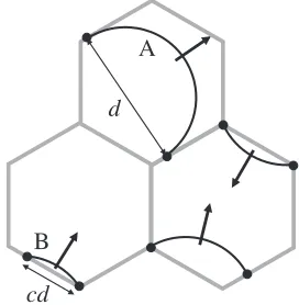
Figure 1 shows the bowing out of perfect dislocations emitted from grain-boundary sources when a shear stress

is applied in the material. If the distance between pinning points is large, such as A in Fig. 1, the dislocation can bow out in a semi-circular shape and becomes the CRSS for the long-range movement of the A dislocation. On the other hand, if the pinning-point distance is small such as B, only a small bow-out is possible and a larger stress is necessary before the B dislocation can take a semi-circular shape.

Statistically speaking, the source lengthL that obeys the condition (5) is randomly distributed on grain boundaries and is a fraction of the grain diameter d so that L¼cd, where cis positive and does not exceed unity. Therefore, we can assume that any pinning-point distanceL, or any value ofc, satisfying the above condition (5) is equally possible; the largerLcauses smallerc.

If the average source lengthhLiis found as a function ofd, insertion of this hLi into L in eq. (3) should give the most probable CRSS for a given d. Then, the problem now is to find the value hLi. This can be done using statistics as follows.

Let us approximatend=as an integer representing the number of potential pinning-point sites at an intersection between a grain boundary and a slip plane. We have

L¼cd¼cn; 0<c<1: ð6Þ

As a simple example, we will first consider the case where equally-spaced (with separation) four (4) potential pinning point sites exist at an intersection line between a grain boundary and a slip plane, as shown in Fig. 2. When a dislocation bows out between any two of the four sites, there are

4C2¼ 4!

2!ð42Þ!¼6 ð7Þ

d

cd

A

B

different ways to choose the two pinning points. Among them, one has the distance3, two have2and three have. Since these six choices are assumed to occur with equal probabilities, the average separationhLibetween the pinning points is calculated as

hLi ¼ð3Þ þ ð22Þ þ ð13Þ

4C2 ¼

5

3: ð8Þ

This analysis can be generalized easily for a grain size of d¼n and the average separation hLi and average coef-ficienthciofcare obtained as

hLi ¼ nþ ðn1Þ2þ ðn2Þ3þ. . .þ1n

nC2

¼nþ2

3 ¼

dþ2

3 ; ð9Þ

hci ¼ hLi

d ¼

nþ2 3n ¼

1þ2ð=dÞ

3 : ð10Þ

The number of grains in a usual UFG tensile specimen is extremely large. In such a case, the average value hLi in eq. (9) is statistically interpreted as the most probable separation between the pinning points. For readers of interest, the statistical interpretation is shown in Appendix.

2.4 Yield stress

From eqs. (3) and (9) together with the Taylor factor M¼3:06, the tensile yield stress y of fcc metals is expressed as

y¼Mc¼

3Mb

2ðdþ2Þln

dþ2

30b

3b

2ðdþ2Þln

dþ2

30b

: ð11Þ

Here, the approximation ofM=1is adopted to obtain the last term. Since all the quantities in eq. (11) are either known or already assigned above ( ¼10nm), we can calculate the values of y and compare them with those obtained in previous experiments. Trial calculations of eq. (11) for b¼0:3nm and 20nm<d <500nm revealed that wide variation offrom 2 nm to 20 nm caused only less than 15% change in the y values. Therefore, we can safely assign

¼10nm for eq. (11) to compare the predicted yield stress with experimental values.

3. Comparison with Previous Studies

3.1 Yield stress

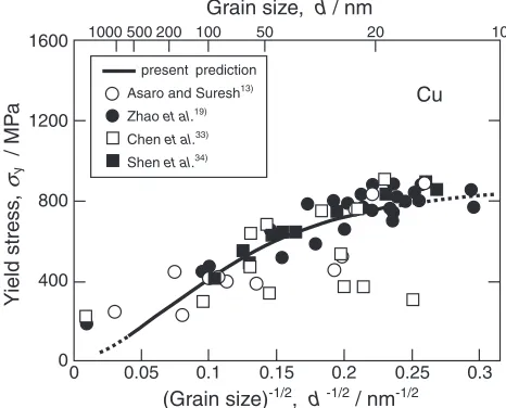
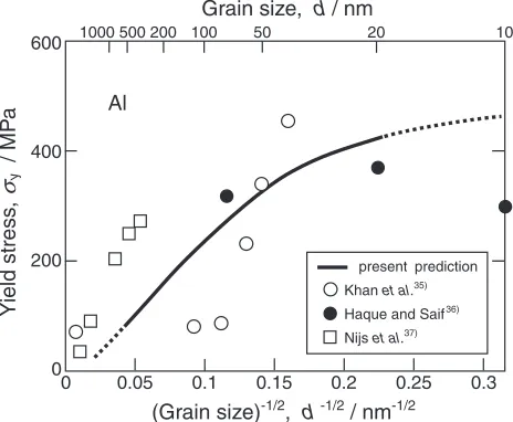
Figures 3, 4 and 5 show the H-P plots of predicted yield stress y from eq. (11) and the experimental data available in the literature for Ni,10,11,32) _Cu13,19,33,34) _{and Al,}35–37) respectively. Constants in eq. (11) used to calculate y are listed in Table 1. Assuming that the yield stress for single crystals of the fcc metals are negligibly small, eq. (11) was used without any additional terms. We can immediately notice from Figs. 3 to 5 that the theoretical curves well reproduce the H-P behaviour at larger grain sizes. The agreement between the model predictions and experimental grain boundary

slip plane

λ

Fig. 2 Equally-separated four pinning points at an intersection between a grain-boundary plane and a slip plane.

Ni

2000

1600

1200

800

400

0

Grain size, d / nm

0 0.05 0.1 0.15 0.2 0.25 0.3

Y

ield stress

,

σy

/ MP

a

(Grain size)-1/2, d -1/2/ nm-1/2

1000 500 200 100 50 20 10

present prediction

Fan et al.10)

Carlton and Ferreira11)

Krasilnikov et al.32)

Fig. 3 Yield stressyas a function of the inverse square root of the grain sizedin Ni. The solid line shows the model prediction of the present study and circles (tensile tests) and squares (hardness tests) are experimental data available in the literature.10,11,32) _{The hardness values Hv were} converted to the yield stress valuesyusing the usual relationHv¼3y.

Cu

Y

ield stress

,

σy

/ MP

a

1600

1200

800

400

0

1000 500 200 100 50 20 10

Grain size, d / nm

0 0.05 0.1 0.15 0.2 0.25 0.3

(Grain size)-1/2_{, d} -1/2_{/ nm}-1/2

present prediction

Asaro and Suresh13)

Zhao et al.19)

Chen et al.33)

Shen et al.34)

data are also reasonably well, at least no worse than any other existing models can predict aside from the empirical H-P straight line. Although the data points for Ni deviate from the theoretical curve for grain sizes smaller than about 20 nm, this is considered to be natural since our model can be applied to the UFG regime of grain size roughly between 20 nm to 500 nm, as mentioned previously.

A similar dislocation bow-out model has been used by Scattergood and Koch to explain the so-called inverse H-P relation.5)As explained earlier, they have adopted the grain size d as the outer cutoff length in the logarithmic term in eq. (1). In the present study, usage of eq. (11) causes a shift in the peak stress towards smaller grain size regions, resulting in the absence of the inverse H-P relation in Figs. 3 to 5. Chenget al.on the other hand, have treated the source length L¼cdin eq. (6) as an adjustable parameter.1)_Ascbecomes larger, the inverse H-P behaviour becomes less significant. They have argued that the source length should become a smaller fraction of the grain size as the grain size increases. However, they could not discuss any further the dependence ofcon the grain size. In the present study, on the contrary, the grain-size dependence ofcwas statistically and analytically incorporated, as shown in eq. (10).

3.2 Strain-rate sensitivity and activation volume It is well known in fcc NC and UFG materials that strain-rate sensitivity exponentmdefined as

m @ln

@ln _""

T

¼ 1

@ @ln _""

T

; ð12Þ

increases as grain size becomes smaller.20,22,29,38–46)_Here, is the flow stress, ""_ the strain rate and T the temperature. Typical values of m at grain sizes d¼20{30nm are m¼

0:03to 0.04 for Cu20,21,28,33,41)_{and 0.01 to 0.02 for Ni.}43,45,46) Since these values are still too small for grain-boundary sliding (m¼0:5) or Coble creep (m¼1), these grain-boundary phenomena are unlikely to be the rate-controlling processes in the UFG regime unless strain rate is very small and/or temperature is high.20,21,34,41,46) Instead, thermally activated dislocation motion to overcome short-range obsta-cles is considered to be more probable in the UFG regime and some possible mechanisms have been proposed. For exam-ple, we find in a recent overview by Dao et al.28) such possible mechanisms as punching of a mobile dislocation through a dense bundle of excess grain-boundary disloca-tions, defect-assisted dislocation nucleation, de-pinning of a dislocation that is pinned at boundary obstacles, etc. All of these mechanisms must also explain a small activation volume in NC and UFG materials as well as the temperature dependence of strength.

As an additional analysis, let us examine what can be said for the thermally activated dislocation process using the present model. The activation volumev_{is written as}

vkT @ln _

@

T

¼M kT @ln _""

@

T

¼M v; ð13Þ

wherekThas its usual meaning,_the shear strain rate,the resolved shear stress andv

the measured activation volume during plastic deformation under uniaxial stress . From eqs. (12) and (13), we have

v¼M kT

m : ð14Þ

The physical meaning ofv_{is the activation areastimes the} Burgers vectorb:

vsb¼ldb; ð15Þ

wherel _{is the length of a dislocation that contributes to a} thermal activation event for overcoming a short-range obstacle and d is the activation distance that scales with the size of the obstacle.

Figure 6 shows a dislocation A that is about to bow out in a semi-circular shape between two pinning points P and Q with separationL. If a thermal activation event occurs locally to overcome the obstacle P, the dislocation A is un-pinned and moves to the position B. Once the configuration B is realized, the curvature of the dislocation A decreases and the long-range motion of the dislocation becomes possible, say, through C and even further. The activation area associated with this unpinning event is defined as the area between the dislocations A and B and is roughly estimated as s

fðL=2Þ bg=2¼Lb=4. Therefore, we have

v¼sb¼Lb2=4¼ ðdþ2Þb2=12; ð16Þ

where the average pinning-point separationhLiin eq. (9) is substituted for L to obtain the last term. From eq. (16) together with ¼10nm, as assumed in section 2.2, we 600

400

200

0

(Grain size)-1/2, d -1/2/ nm-1/2

0 0.05 0.1 0.15 0.2 0.25 0.3

Al

1000 500 200 100 50 20 10

Grain size, d / nm

Y

ield stress

,

σy

/ MP

a

present prediction

Khan et al.35)

Haque and Saif36)

Nijs et al.37)

Fig. 5 Yield stressyas a function of the inverse square root of the grain sizedin Al. The solid line shows the model prediction of the present study and circles are experimental data available in the literature.35–37)_{The data} by Nijset al.37)_{are for an Al-Mg alloy.}

Table 1 Values for constants used to calculateyfrom eq. (11).

Ni Cu Al

Shear modulus,

/GPa 76 48 26

Burgers vector,

b/nm 0.249 0.255 0.284 Source length,

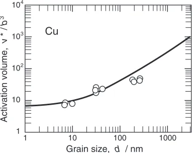
can obtain the grain-size dependence of the activation volume. The curve in Fig. 7 shows the calculated activa-tion volume as a funcactiva-tion of grain size for Cu. The data points (circles) in the figure were taken from the exper-imental results summarized by Chenet al.33)As can be seen, the agreement between the theory and experiment is excellent.

A similar plot formis possible by using eqs. (11), (14) and (16), as shown in Fig. 8. To draw the curve, M¼pffiffiffi3 was assigned in eq. (14). This assignment is merely for the purpose of comparison with the experimental results (circles in Fig. 8) summarized by Chenet al.33)_{who usedM¼}pffiffiffi_3in their analysis. We again find the excellent agreement.

4. Concluding Remarks

From the present study, we have found that the dislocation bow-out model can reasonably explain not only the observed strength but also the grain-size dependence of the activation volume and strain-rate sensitivity. During the course of this study, the H-P relation was not used nor postulated. This may indicate that the observed H-P relation is just fortuitous and it is not a prerequisite for the deformation mechanism of NC

and UFG materials. Further study is necessary to reveal the grain boundary contribution to the strength.

Our discussion on the thermally activated dislocation mo-tion in Secmo-tion 3.2 is incomplete in a sense that the original equation of strength (eq. (11)) was derived without taking into account the kinetics of deformation. Even if the present de-pinning process does determine the strain-rate sensitivity of UFG materials, a thermal activation event at a given temperature should occur before a dislocation takes a semi-circular shape. Therefore, more rigorous discussion based on the kinetics of plastic deformation is needed. Nevertheless, it is interesting to find that the present study can explain the observed dependencies of strain-rate sensitivity and activa-tion volume on grain size. We believe research along this line will reveal whether or not the present analysis is really applicable as a strength mechanism of the UFG materials.

Acknowlegment

This research was supported by a Grant-in-Aid for Scientific Research on Priority Areas (18062002) by the Ministry of Education, Culture, Sports, Science and Tech-nology of Japan.

Appendix

Let L(¼;2;3;. . .;n) be a random variable and its distribution function be described asPðLÞ. For our problem of grain size d¼n,L is the group of all the possible source length andPðLÞmeans its frequency of appearance, as shown in Fig. A·1. WhenhLidenotes the average (expectation) ofL, we have from eq. (9)

hLi ¼ ðnþ2Þ=3: ðA:1Þ

On the other hand, the variance2 _{ofPðLÞis defined as}47)

2 hðL hLiÞ2i ¼ hL2i hLi2: ðA:2Þ

Since

hL2i ¼ 2

2

nðnþ1Þ½1 2

nþ22 ðn1Þ

þ32 ðn2Þ þ. . .þn2 fn ðn1Þg

b

L/2

A B C

boundary pinning point

P Q

Fig. 6 When the bowing-out dislocation A pinned at boundary obstacles P and Q overcomes the obstacle P by thermal activation, the dislocation A moves locally to B. Then, the dislocation can automatically move to C and further to cause long-range motion. The activation volume for this event is defined as Bergers vector times the activation area bounded by dislocations A and B.

1 10 100 1000 104

103

102

10

1

Grain size, d / nm

Activation volume,

v

*

/

b

3

Cu

Fig. 7 Predicted grain size dependence of the activation energy of UFG Cu calculated from eq. (16). The data points are taken from the paper by Chen

et al.33)

0.08

0.06

0.04

0.02

0

1 10 100 1000 Grain size, d / nm

Strain-rate sensitivity,

m

Cu

¼ 2 2

nðnþ1Þ n

Xn k¼1

k2X

n1

k¼1

kðkþ1Þ2

" #

¼ðnþ1Þðnþ2Þ

6

2

; ðA:3Þ

the variance can be calculated as

2 ðn1Þðnþ2Þ

18

2_{: ðA:4Þ}

As a next step, let us consider that N random variables L1;L2;. . .;LN with the same PðLÞ and the same average of (A·1) exist. In our problem, N is the number of grains (all with the same grain size) in a specimen. The central limit theorem in statistics shows that whenNis much larger than unity, the difference betweenhLiin eq. (A·1) and the sample average defined asðL1þL2þ. . .þLNÞ=N obeys a normal distribution function with the average zero and the variance

2_{=N. For example, if an UFG specimen with d¼100nm} (n¼10for¼10nm) has a volume of 1 mm3_{, the number} of grains in the specimen is approximately N1012_. Therefore, the standard deviation (square root of the variance) can be calculated from eq. (A·4) as ð2=NÞ1=2

2:4106. Since this value is much smaller thanhLi ¼4

from eq. (A·1), the normal distribution of the sample average is highly concentrated around hLi and by far the most probable value.

REFERENCES

1) S. Cheng, J. A. Spencer and W. W. Milligan: Acta Mater.51(2003) 4505–4518.

2) A. H. Chokshi, A. Rosen, J. Karch and H. Gleiter: Scr. Metall.23

(1989) 1679–1684.

3) T. G. Nieh and J. Wadsworth: Scr. Metall. Mater.25(1991) 955–958. 4) G. E. Fougere, J. R. Weertman, R. W. Siegel and S. Kim: Scr. Metall.

Mater.26(1992) 1879–1883.

5) R. O. Scattergood and C. C. Koch: Scr. Metall. Mater. 27(1992) 1195–1200.

6) C. C. Koch and J. Narayan: Mater. Res. Soc. Sym. Proc.634(2001) B5.1.1.

7) S. Takeuchi: Scr. Metall. Mater.44(2001) 1483–1487. 8) J. Schiotz and K. Jacobsen: Science301(2003) 1357–1359. 9) H. Conrad and K. Jung: Mater. Sci. Eng. A391(2005) 272–284. 10) G. J. Fan, H. Choo, P. K. Liaw and E. J. Lavernia: Mater. Sci. Eng. A

409(2005) 243–248.

11) C. E. Carlton and P. J. Ferreira: Acta Mater.55(2007) 3749–3756. 12) R. J. Asaro, P. Krysl and B. Kad: Phil. Mag. Lett. 83 (2003)

733–743.

13) R. J. Asaro and S. Suresh: Acta Mater.53(2005) 3369–3382. 14) B. Zhu, R. J. Asaro, P. Krysl and R. Bailey: Acta Mater.53(2005)

4825–4838.

15) V. Yamakov, D. Wolf, M. Salazar, S. R. Phillpot and H. Gleiter: Acta Mater.49(2001) 2713–2722.

16) V. Yamakov, D. Wolf, S. R. Phillpot, A. K. Mukherjee and H. Gleiter: Nature Mater.1(2002) 45–49.

17) D. A. Hughes and N. Hansen: Acta Mater.48(2000) 2985–3004. 18) N. Hansen, X. Huang and D. A. Hughes: Mater. Sci. Eng. A317(2001)

3–11.

19) M. Zhao, J. C. Li and Q. Jiang: J. Alloys Compd. 361 (2003) 160–164.

20) Q. Wei, S. Cheng, K. T. Ramesh and E. Ma: Mater. Sci. Eng. A381

(2004) 71–79.

21) S. Cheng, E. Ma, Y. M. Wang, L. J. Kecskes, K. M. Youssef, C. C. Koch, U. P. Trociewitz and K. Han: Acta Mater.53(2005) 1521–1533. 22) A. S. Argon and S. Yip: Phil. Mag. Lett.86(2006) 713–720. 23) H. Petryk and S. Stupkiewicz: Mater. Sci. Eng. A 444 (2007)

214–219.

24) J. C. M. Li: Trans. Metall. Soc. AIME227(1963) 239–247. 25) A. Mascanzoni and G. Buzzichelli: Phil. Mag. A22(1970) 857–860. 26) L. E. Murr: Metall. Mater. Trans. A6(1975) 505–513.

27) F. Spaepen and D. Y. W. Yu: Scr. Mater.50(2004) 729–732. 28) M. Dao, L. Lu, R. J. Asaro, J. T. M. De Hosson and E. Ma: Acta Mater.

55(2007) 4041–4065.

29) J. Weertman and J. R. Weertman: Elementary Dislocation Theory, (Macmillan, New York, 1964).

30) F. R. N. Nabarro:Theory of Crystal Dislocations, (Oxford University Press, Oxford, 1967).

31) J. P. Hirth and J. Lothe:Theory of Dislocations, 2nd ed., (John Wiley and Sons, Inc., New York, 1982).

32) N. Krasilnikov, W. Lojkowski, Z. Pakiela and R. Valiev: Mater. Sci. Eng. A397(2005) 330–337.

33) J. Chen, L. Lu and K. Lu: Scr. Mater.54(2006) 1913–1918. 34) Y. F. Shen, L. Lu’, Q. H. Lu, Z. H. Jin and K. Lu: Scr. Mater.52(2005)

989–994.

35) A. S. Khan, Y. S. Suh, X. Chen, L. Takacs and H. Zhang: Int. J. Plasticity22(2006) 195–209.

36) M. A. Haque and M. T. A. Saifp: Scr. Mater.47(2002) 863–867. 37) O. Nijs, B. Holmedal, J. Friis and E. Nes: Mater. Sci. Eng. A, (2008)

in press.

38) F. Dalla Torre, H. Van Swygenhoven and M. Victoria: Acta Mater.50

(2002) 3957–3970.

39) Y. M. Wang and E. Ma: Appl. Phys. Lett.83(2003) 3165–3167. 40) R. Schwaiger, B. Moser, M. Dao, N. Chollacoop and S. Suresh: Acta

Mater.51(2003) 5159–5172.

41) Y. M. Wang and E. Ma: Mater. Sci. Eng. A375–377(2004) 46–52. 42) J. May, H. W. Ho¨ppel and M. Go¨ken: Scr. Mater.53(2005) 189–194. 43) F. Dalla Torre, P. Spa¨tig, R. Scha¨ublin and M. Victoria: Acta Mater.53

(2005) 2337–2349.

44) F. H. Dalla Torre, E. V. Pereloma and C. H. J. Davies: Acta Mater.54

(2006) 1135–1146.

45) L. Hollang, E. Hieckmann, D. Brunner, C. Holste and W. Skrotzki: Mater. Sci. Eng. A424(2006) 138–153.

46) Y. M. Wang, A. V. Hamza and E. Ma: Acta Mater. 54 (2006) 2715–2726.

47) M. Dwass:Probability: Theory and Alppications, (W. A. Benjamin, Inc., New York, 1970).

λ

λ

λ

λ

λ

n-1

n-2

n-3

1

0

Random variable, L

Distribution function,

P

(

L

)

. . .

. . .