Application of Factor and Cluster Analysis for an evaluation of Business Practices Models of Foreign Banks

Munich Personal RePEc Archive

Application of Factor and Cluster

Analysis for an evaluation of Business

Practices Models of Foreign Banks.

Edurkar, Ashok and Chougule, Dr.Dattatrya G.

Commerce Management Department, Shivaji University Kolhapur,

India

14 July 2016

Online at

https://mpra.ub.uni-muenchen.de/73536/

Title of Research Paper:-

Application of Factor and Cluster Analysis for an

evaluation of Business Practices Models of Foreign

Banks Post RBI Road MAP 2005 and during the period

2003 to 2013 with reference to India’s Foreign Trade.

Author's name: Mr.Ashok Edurkar, Dr. Dattatrya

G.Chougule

First Author’s Designation: - Management Consultant,

Stork International GmbH, Vienna, Austria

Research Centre Name: - Commerce & Management

Department Shivaji University Kolhapur, Maharashtra

State.

First Author’s Postal address: - 35, Ganga Vishnu

Heights, Near Alankar Police Station, Karvenagar Pune,

PIN-411052

Application of Factor and Cluster Analysis for an evaluation of

Business Practices Models of Foreign Banks Post RBI Road MAP

2005 and during the period 2003 to 2013 with reference to India’s

Foreign Trade.

Abstract-

The aim of this paper is to assess business practices models of 24 foreign

banks operating in India post RBI Road Map 2005 and during the period 2003 to 2013

through the use of publicly available information. Business practices models have

been evaluated by the application of factor analysis followed by cluster analysis. 23

variables related to working of foreign banks supported with 5 variables related to

India’s foreign trade were reduced into 8 factors by using factor analysis. Using these

8 factors cluster analysis was carried out to group 24 foreign banks into 3 clusters

leading to three distinct business practices models. The dataset for analysis was for

the period for financial years 2003-04 to 2012-13 and the focus is on post RBI Road

Map-2005 for foreign banks.The foreign banks’ sample consists of consistently operating 24 number foreign banks out of the universe consisting of 43 FBs operating

in India between 2003-04 and 2012-13(ten years observation period).This study

broadly covers foreign banks having legal entity and financial roots primarily in home

country and entered in India for tapping Indian financial market in the form of term

loans, cash credit, bridge loans, investments and funding for business activities

(business financing operations) .

Key Words- Foreign Banks, Finance, Models, Foreign Trade, Financing

1Introduction: - Foreign banks are developing their Indian business along with

increasing their client base and implementing potential opportunities for massive entry

into the market. Most of the foreign banks have the greatest experience in working with

private depositors, and also lending actively to the real and various business sectors.

Foreign banks desire to enter the Indian market is understandable. Bilateral trade with

various countries has been growing rapidly as economies are recovering from the global

financial crisis. Foreign banks’ principal focus is on promoting bilateral trade by offering finance at various stages of business cycle like product development,

production, and marketing, import-export credit at pre-shipment and post-shipment

stages, investment abroad and import of technology. Foreign banks operate a wide

range of lending programs. Financial packages offered by the Foreign banks are

economy. It is the dominant provider of capital in the form of advances & investments

to various sectors like construction, automobile, energy, machinery industry covering

also priority sectors including agriculture, MSE, weaker section and exports plus

imports.

1.1 Foreign banks’ their Current Scenario: - During the last two decades, India has seen an unprecedented degree of globalization especially in financial services. Foreign

trade, financial system, technological advances, deregulation impact, industry and its

major players’ growth were identified as industry shaping milestones that gradually

formed the today’s foreign banks’ models. As of March 2013, there are 43 foreign banks from 26 countries operating as branches and 43 foreign banks from 22 countries

operating as representative offices in India. In addition, a number of foreign banks have

also entered India via the Non-Banking Financial Company (NBFC) route, while a

considerable number have set up captive centers in the country.

1.2 Significance of study: - Knowing under what models foreign banks operate for

financing India’s Foreign Trade and how models change in perspective to time or the foreign banks’ operative approach can provide valuable insight into the whole financial

system. Foreign banks are to develop commercially viable relationships with a target

set of externally business oriented companies in India and their host countries by

offering them comprehensive range of products and services, aimed at enhancing their

internationalization efforts with the application of specific models.

1.3 Criticism against foreign banks: - It is observed that foreign banks operating in

various developing countries are focused on a section of credit worthy customers and

are involved in taking out cream of credit market. While carrying out financing

operations these institutions in general neglect small or marginal customers. (Mandira

Sarma and Anjali Prashad 2014). It has become hard to forecast, monitor or even follow

how foreign banks conduct their business.

1.4 Foreign banks andRural Regions in India: - It is argued that the developmental

needs of rural regions in India may not be met by foreign banks. In India, out of

approximately 600 districts, the number of districts without financial facility is nearly

400. Foreign banks are not going to enhance the reach of the financial system to millions

of rural Indians manufacturers/service providers / businesses /citizens who do not have

2. Research Methodology: -

2.1 This research study is mainly based on secondary data.

2.1.1 First of all published literature relating to the Foreign Trade of India and financing

of Foreign Trade was collected and consulted with special reference to FBs.

2.1.2 Secondly full advantage was taken of consultation with the faculty of various

institutes related to Foreign Trade. For example, Indian Institute of Foreign Trade

(IIFT), EXIM Bank, NIBM, Foreign Trade Organizations, Commerce wing in Indian

High Commissions in various countries.

2.1.3 Thirdly a broad view was obtained on the role of FBs on the growth of Foreign

Trade of India and financial models applied by FFIs while operating in India.

2.1.4 Lastly an analysis of the total operations of the FBs and their functional variables

will be undertaken to find out how far FBs are able to achieve their objectives.

2.2 Data and Source of Data:-

The present study is predominantly empirical in nature and based on secondary

data. This study involved basically published literature searches and various internet

web site searches related to Foreign Trade and Foreign banks for obtaining secondary

data.

2.3 Sample Design & selection of FFIs:-

For this study foreign banks are selected by random sampling method but belong to

major countries related to India’s Foreign Trade, a home country of foreign banks having a sizable bilateral trade with India and non-interrupted operation as indicated by

profile of banks as per RBI.

2.4 Sampling Plan:

A sample of 24 FBs is selected among 43 FBs (Universe) satisfying various conditions

as per sampling design. This corresponds to (24/43) = 55.81 % of total universe value.

The study is conducted on the FBs operating in India during the financial year 2003-04

to 2012-13.

2.5 Data analysis techniques:-

For effective analysis of data secondary data, various statistical tools like trend analysis,

averages, etc. software like IBM SPSS are used. Data analysis activity begins with

the period 2003-04 to 2012-13. This is processed for calculation of Mean, Standard

Deviation, Min, Max, Standard Error etc. The processed data is used to generate input

for factor and cluster analysis.

2.6:-Scope of the Study:-This study broadly covers foreign banks having legal entity

and financial roots primarily in home country and entered in India for tapping Indian

market in the form of term loans, cash credit, bridge loans, equity participation and

funding for business activities .

2.7 Limitations of the Study: - This study is limited to determination of effect of

funding by foreign banks to Indian businesses/manufacturing/service operations and

trading involving term loan or cash credit in the form of advances.

3.1 Review of Literature in short:-

The foreign banks model analysis offers a wide range of applications. Several authors

already employed this type of analysis, generating promising results. The concept is

used as an educative and analytical tool to explain and understand how foreign banks

function. The term model is widely applied and capable of including a range of financial

business aspects. Financial business objectives, core customers, product management,

financial business strategies, organization infrastructure and many other strategic and

operational business processes fit in foreign banks model term. Because of this

capability to explain so much, foreign banks model term suffers an “identity crisis”. While scholars do not agree what a model is, certain patterns are available and

definitions emerge (Pedrotti (2014)) and (Osterwalder, Pigneur 2010). For the purpose

of a more tangible applicability and necessary foreign banks model comparability, a

work by Zott and Amit is used as a definition core for the model (Zott, Amit 2008).

Applying similar conceptualization in the foreign bank business, the acquisition of

necessary funds, loan service provisions and implied risk-taking can be interpreted as a

base financial product market strategy, as these are the same products/services that

foreign banks are competing for in the financial market The evolutionary logic of the

foreign bank model is addressed by sympathizing with G. George’s and A. Bock’s thinking that organizations adjust and redesign their models under the effects of a

changed operational environment (George, Bock 2011). The ability to adjust or

transform the model is regarded as one of the major features in the financial business

3.2 Research Gap Analysis:-

3.2.1 Scope of Review: - The effect of opening of economy on growth of a country and

various models of foreign bank has been critically covered. In general, researchers point

out that foreign bank is an important factor for the GDP growth. Openness to foreign

banks policy yields access to finance at a competitive rate.

3.2.2 Limitations of Review: - The effect of external financing from foreign banks on

working of domestic institutions is not examined. There is no unanimous acceptance

amongst researchers about specific models of foreign banks operating in host and home

countries.

3.2.3 Scope for further review work: - Effect of external financing from foreign banks

on working of domestic institutions may be reviewed in detail along with priority sector

financing.

4.1 Analysis and Interpretation of

Data:-World over no bank is confined to a specific theoretical model. Although institutions

operating in Europe, such as BNP Paribas, Deutsche Bank or Société Générale define

themselves as retail-oriented institutions for marketing purposes, the research provides

evidence that their business model is in fact closer to investment banking (Ayadi et.al.

2012). Similarly, the 24 selected foreign banks operating in India, are not relying on

any specific theoretical model but making use of best of all business opportunities

available.

4.2 Profile of selected foreign banks for study purpose and variables

4.2.1 During the year2003-04 to 2012-13 (ten years observation period) there are only

twenty four of FFIs operating consistently in India. These foreign banks are selected

for this research to generate models of foreign banks.

Annexure-1shows the details of these twenty four foreign banks including their

respective case number allotted along with business, advances, investment.

4.2.2 Annexure-2 shows List of Variables and Factor/Component Score Coefficient

Matrix.

4.2.3 The analysis for Foreign Trade Variables, is conducted using annual data for each foreign bank operating in India.

Based on the above, case wise calculation of values of eight factors was performed which served as an input for conducting cluster analysis to yield three clusters which are termed as Model-A, Model-B and Model-C. Annexure-3 Case wise calculations of values of 8 number factors.

4.3Five variables pertaining to foreign trade: - These are derived based on gravity equations used in the research of foreign trade. The variables included in the export and import volume equations are real exports contribution by foreign bank, real imports contribution by foreign bank , real gross domestic product contribution by foreign bank (CTGDP ), Modified export demand (M-EXDEM) because of foreign bank, and trade finance (FIN). For the export volume equation, export demand represents market share and is computed as the ratio of imports to total exports, specifically

M-EXDEM = Sum of 𝑖𝑚𝑝𝑜𝑟𝑡𝑠 /Sum of 𝑒𝑥𝑝𝑜𝑟𝑡𝑠 (4.3.1)

Where 𝑖𝑚𝑝𝑜𝑟𝑡𝑠 is considered total imports into India.

𝐸𝑥𝑝𝑜𝑟𝑡𝑠 represents total exports to all countries by India.

To examine how financial development and foreign trade finance influence trade flows, econometric models similar to those found in Arize (1996), Asafu-Adjeye (1999), and Ozturk and Kalyoncu (2009) were referred. Also, research work by Daniel Perez Liston, Lawrence McNeil (2013) was referred.

The proposed export volume equation is as follows:

Log (𝑒𝑥𝑝𝑜𝑟𝑡𝑠) = A0 +A1log (M-𝐸𝑋𝐷𝐸𝑀) + A2𝐹𝐼𝑁 +A3𝐹𝐼𝑁 (4.3.2)

Where exports are real exports contribution by foreign bank, M-EXDEM is a proxy for export demand contribution by foreign bank, FIN is the trade finance proxy contribution by FFI. Now, Imports are modeled as follows:

Log (𝑖𝑚𝑝𝑜𝑟𝑡𝑠) = A0 +A1log (M𝐺𝐷𝑃) +A2𝐹𝐼𝑁 (4.3.3)

Where imports, are real imports contribution by foreign bank and M-GDP is the real gross domestic product contribution by foreign bank. A0, A1, A2 are constants. From profile of foreign banks it is observed that foreign banks’ Business is equal to number of Employees multiplied by Business per Employee. The definition of Proposed Modified Formulae for Foreign Trade Variables are as follows:-

(A) M-EXDEM =Modified variable for export demand as per foreign bank’s

financing= (Total Imports/Total Exports)*(Investments by foreign bank)*(Advances

by foreign bank) where, (foreign bank’s Business) = ('No. of Employees* 'Business /Employee')

(C) EIR=Effective Interest Rate ==100*(Interest Income by foreign bank/Advances by foreign bank)

(D) Log (M-FT) =Log ((((Average FT)/ (Investments!*Advances!)))

(E) Log (CTGDP) =Log ((Investments!*Advances!)*('No. of Employees'!*'Business

per Employee'!))

Based on the above definition values of foreign trade variables have been computed

and used in working of factor analysis followed by cluster analysis.

4.4 Scree plot graph:-The scree plot graphs the eigen value against the factor number.

Graph 4.4.1:- Scree plot graph:-

Graph 4.4.1 shows Eigen values which are given in the first two columns of the table

number 5.6 immediately above. From the eighth factor on, it is observed that the line

is almost flat, meaning the each successive factor is accounting for smaller and smaller

amounts of the total variance.

For determining the number of factors to retain we have used Cattell’s (1966) scree test, which involves eye-balling the plot of the eigenvalues for a break or hinge (also referred

to as an “elbow”). The rationale for this test is based on the idea that a few major factors

will account for the most variance, resulting in a “cliff”, followed by a shallow “scree”

depicting the consistently small and relatively shallow error variance described by

minor factors. Annexure- 2 indicates Component Score Coefficient Matrix. For a

wise values of factors 1 to 8. Annexure 3 shows mean or average values of variables

for the period 2003-04 to 2012-13. For example, for the variable ‘Advances’ the value of Factor 1 is 0.06. For case 1, the mean value for Advances is 0.07515. Then for the

case 1, the value of Factor1 for a variable ‘Advances’ is equal to 0.06 multiply 0.07515= 0.004509. Using this method, the value of Factor1 is calculated for all variables 1 to 28

and the sum of these values is the value of Factor1 for case1. These case wise values of

factors 1 to 8 are given in Annexure-4.

4.5 Cluster analysis:-

For this research study, cluster analysis is carried out as follows:-

4.5.1 Case (Foreign bank) wise computation of values of 8 factors which are generated

using factor analysis.

4.5.2 Case (Foreign bank) wise calculation and recording of 8 factors in tabular format.

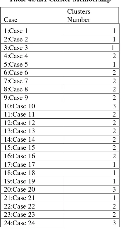
After processing the data for Cluster Analysis using SPSS, details related to Cluster

[image:10.595.213.420.370.762.2]

Membership are as under:-

Table 4.5.2.1 Cluster Membership

Case

Clusters Number

1:Case 1 1

2:Case 2 1

3:Case 3 1

4:Case 4 2

5:Case 5 1

6:Case 6 2

7:Case 7 2

8:Case 8 2

9:Case 9 2

10:Case 10 3

11:Case 11 2

12:Case 12 2

13:Case 13 2

14:Case 14 2

15:Case 15 2

16:Case 16 2

17:Case 17 1

18:Case 18 1

19:Case 19 1

20:Case 20 3

21:Case 21 1

22:Case 22 2

23:Case 23 2

[image:11.595.86.449.381.689.2]

Table 4.5.2.1 shows to which cluster a particular case is belonging. For example, case

number 17 is in cluster number 1, case number 13 is in cluster number 2 and case

number 24 is in cluster number 3.

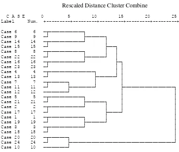
Graph 4.5.1 shows “Dendrogram”. In Greek language the word ‘ Dendro’ means tree.

Here the cases in 3 number clusters are presented in a ‘Tree shape’ or called as a

Dendrogram. The branching-type-nature of the Dendrogram allows the researcher to

trace backward or forward to any individual case or cluster at any level. It, in addition,

gives an idea of how great the distance was between cases or groups that are clustered

in a particular step, using a 0 to 25 scale along the top of the chart. While it is difficult

to interpret distance in the early clustering phases (the extreme left of the graph), as you

move to the right relative distance become more apparent. The bigger the distances

before two clusters are joined, the bigger the differences in these clusters. To find a

membership of a particular cluster simply trace backwards down the branches to the

name.

Graph 4.5.1 Dendrogram using Centroid Method

Rescaled Distance Cluster Combine

C A S E 0 5 10 15 20 25 Label Num. +---+---+---+---+---+

Case 6 6 ─┬─────────────┐

Case 9 9 ─┘ ├───────┐ Case 14 14 ─┬─────────────┘ │ Case 15 15 ─┘ ├───┐ Case 8 8 ─┬─────────────┐ │ │ Case 22 22 ─┘ ├───────┘ │ Case 16 16 ─┬─────────────┘ ├─┐ Case 23 23 ─┘ │ │ Case 4 4 ─┬─────────────────┐ │ │ Case 13 13 ─┘ ├───────┘ │ Case 7 7 ─┬───────┐ │ │

Case 11 11 ─┘ ├─────────┘ ├───────────────────┐ Case 12 12 ─────────┘ │ │ Case 5 5 ─┬─────────────┐ │ │ Case 21 21 ─┘ ├───────┐ │ │ Case 2 2 ─┬─────────────┘ │ │ │ Case 17 17 ─┘ ├─────┘ │ Case 1 1 ─┬─────────────┐ │ │ Case 19 19 ─┘ ├───────┘ │ Case 3 3 ─┬─────────────┘ │ Case 18 18 ─┘ │ Case 20 20 ─┬───────┐ │ Case 24 24 ─┘ ├───────────────────────────────────────┘ Case 10 10 ─────────┘

4.6 Characteristics of Foreign Banks’- 3 Models: - This part of the research determines and discusses specific characteristics of the three models derived by the

are expressed in terms values of eight factors which are either positive or negative

values.

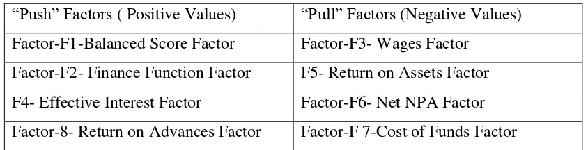
4.6.1 Identification of Factors based on positive or negative scores: - Two distinct

groups of all 8 factors are formed based on positive or negative value of factors with

respect to 24 cases used in this research. Positive values are considered as positive push

and negative values are considered as negative pull for the operational activities of

foreign banks.

Table 4.6.1 Identification of Factors based on positive /negative scores

“Push” Factors ( Positive Values) “Pull” Factors (Negative Values) Factor-F1-Balanced Score Factor Factor-F3- Wages Factor

Factor-F2- Finance Function Factor F5- Return on Assets Factor

F4- Effective Interest Factor Factor-F6- Net NPA Factor

Factor-8- Return on Advances Factor Factor-F 7-Cost of Funds Factor

4.6.2 Absolute Mean Values:-These values are actual or real mean values of eight

factors with respect to specific Model either Model-A or model-B or Model-C. Models

are segregated based on ascending order of mean values. Table 5.35 indicates ascending

order of Models A to B to C and also furnishing mean values of eight factors with

[image:12.595.105.527.235.343.2]

respect to specific model.

Table 4.6.2 Absolute Mean Values:-

Model

F1

F2

F3

F4

F5

F6

F7

F8

A 1190.752 114.5553

-218.467

560.8069

-142.191

-569.374 -570.518 549.0386

B 11419.46 991.8395

-1746.84

5168.439

-749.443

-5498.83 -5081.52 5539.352

C 119204.2 9457.528

-25604.8

53612.01

-14242.7

-60862.1 -59923.1 34007.19

4.6.3 Percentage Values: - These values are percentage of mean values of eight factors

with respect to specific Model either Model-A or model-B or Model-C. Models are

order of Models A to B to C and also furnishing percentage of mean values of eight

factors with respect to specific model Table 4.6.3 Percentage Mean Values

Model

F1

F2

F3

F4

F5

F6

F7

F8

A 0.903 1.084 0.792 0.945 0.939 0.850 0.870 1.369

B 8.663 9.388 6.335 8.709 4.951 8.215 7.749 13.815

C 90.43 89.52 92.87 90.345 94.108 90.933 91.380 84.815

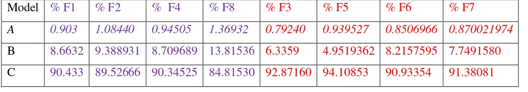
4.6.4 Grouping of Factors based on Positive Push & Negative Pull is carried out based

on positive value or negative value of absolute mean value of factors and further

converting it into percentage value. Table 4.6.4 shows above mentioned grouping.

Factor F1, F2, F4 F8 represent Positive Push group whereas Factor F3, F5, F6, F7

represent Negative Pull group. Models are placed in ascending order of percentage

[image:13.595.25.542.415.505.2]

values of eight factors.

Table 4.6.4 Grouping of Factors based on Positive Push / Negative Pull: - Positive

Push is in blue color whereas Negative Pull is in red color

Model % F1 % F2 % F4 % F8 % F3 % F5 % F6 % F7

A 0.903 1.08440 0.94505 1.36932 0.79240 0.939527 0.8506966 0.870021974

B 8.6632 9.388931 8.709689 13.81536 6.3359 4.9519362 8.2157595 7.7491580

C 90.433 89.52666 90.34525 84.81530 92.87160 94.10853 90.93354 91.38081

4.6.5 Model A: - This is basically cluster 1. It includes eight cases out of 24 cases

analyzed during the research. Table 4.6.5 indicates eight cases along with values of

eight factors with respect to specific case. This table also shows maximum values,

minimum values, mean value and value of standard deviation of eight factors with

respect to cases involved in this research. Here, both absolute mean values and

percentages mean values of eights factors are at the minimum or the least level. Hence

this model is termed as “Also Ran Low End Economy model” of the foreign banks,

meaning foreign banks covered under this model are just maintaining their existence by

carrying out their operational activities while operating in India. These foreign banks

lack initiative to tap various business opportunities available under the RBI roadmap

with the application of variables like advances, investment, EIR etc.to widen their

Table 4.6.5 Model A – 8 Cases Case No. Factor- F1 Factor- F2 Factor- F3 Factor- F4 Factor- F5 Factor- F6 Factor- F7 Factor- F8

1 153.19 15.65 -8.74 93.12 -7.61 -55.33 -66.94 101.85

2 1454.31 142.33

-397.18

698.33

-323.27

-758.98 -816.36 267.57

3 831 77.16

-110.63

373.25 -0.37 -353.76 -354.63 781.64

5 1098.7 101.91

-239.53

514.67

-181.21

-549.23 -564.5 327.67

17 1681.87 166.83

-302.51

792.36

-181.97

-809.67 -812.95 867.27

18 3051.33 283.78

-489.79

1407.18

-299.84 -1452.44 -1363.34 1360.89

19 70.58 5.77 7.55 50.89 -16.47 -24.49 -41.6 5.31

21 1185.04 123

-206.89

556.66 -126.8 -551.09 -543.83 680.11

Max 3051.33 283.78 7.55 1407.18 -0.37 -24.49 -41.6 1360.89

Min 70.58 5.77

-489.79

50.89

-323.27 -1452.44 -1363.34 5.31

Mean 1190.75 114.56

-218.47

560.81

-142.19

-569.37 -570.52 549.04

S.Deviation 883.29 83.21 165.79 403.88 119.9 430.39 407.51 426.54

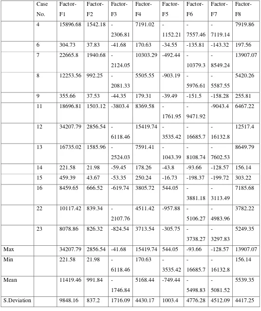
4.6.6 Model B: - This is basically cluster 2. It includes thirteen cases out of 24 cases

analyzed during the research. Table 4.6.6 indicates thirteen cases along with values of

eight factors with respect to specific case. This table also shows maximum values,

minimum values, mean value and value of standard deviation of eight factors with

respect to cases involved in this research. . Here, both absolute mean values and

percentages mean values of eights factors are at the moderate or the medium level.

Hence this model is termed as “Progressive Medium End model” of the foreign banks,

meaning foreign banks covered under this model are pushing their presence by carrying

out their operational activities while operating in India. These foreign banks possess

the application of variables like advances, investment, EIR etc.to widen their

[image:15.595.12.548.133.772.2]

prospective customer base and increase income plus appropriate profitability.

Table 4.6.6 Model B- 13 Cases

Case No. Factor- F1 Factor- F2 Factor- F3 Factor- F4 Factor- F5 Factor- F6 Factor- F7 Factor- F8

4 15896.68 1542.18

-2306.81

7191.02

-1152.21 -7557.46 -7119.14 7919.86

6 304.73 37.83 -41.68 170.63 -34.55 -135.81 -143.32 197.56

7 22665.8 1940.68

-2124.05

10303.29 492.44

-10379.3

-8549.24

13907.07

8 12253.56 992.25

-2081.33

5505.55 903.19

-5976.61

-5587.55

5420.26

9 355.66 37.53 -44.35 179.31 -39.49 -151.5 -158.28 255.81

11 18696.81 1503.12 -3803.4 8369.58

-1761.95

-9471.92

-9043.4 6467.22

12 34207.79 2856.54

-6118.46

15419.74

-3535.42 -16685.7 -16132.8 12517.4

13 16735.02 1585.96

-2524.03

7591.41

-1043.39 -8108.74 -7602.53 8649.79

14 221.58 21.98 -59.45 178.26 -43.8 -93.66 -128.57 156.14

15 459.39 43.67 -53.35 250.24 -16.73 -198.37 -199.72 303.22

16 8459.65 666.52 -619.74 3805.72 544.05

-3881.18

-3113.49

7185.68

22 10117.42 839.34

-2107.76

4511.42 957.88

-5106.27

-4983.96

3782.22

23 8078.86 826.32 -824.54 3713.54 305.75

-3738.27

-3297.83

5249.35

Max 34207.79 2856.54 -41.68 15419.74 544.05 -93.66 -128.57 13907.07

Min 221.58 21.98

-6118.46

170.63

-3535.42 -16685.7 -16132.8 156.14

Mean 11419.46 991.84

-1746.84

5168.44 749.44

-5498.83

-5081.52

5539.35

4.6.7 Model C: - This is basically cluster 3. It includes three cases out of 24 cases

analyzed during the research. Table 4.6.7 indicates three cases along with values of

eight factors with respect to specific case. This table also shows maximum values,

minimum values, mean value and value of standard deviation of eight factors with

respect to cases involved in this research. Here, both absolute mean values and

percentages mean values of eights factors are at the maximum or at the highest level.

Hence this model is termed as “High End Star model” of the foreign banks, meaning foreign banks covered under this model are leaving no chance for pushing their

presence at the highest level by carrying out their operational activities while operating

in India. These foreign banks possess proactive initiative to tap various business

opportunities available under the RBI roadmap with the application of variables like

advances, investment, EIR etc.to widen their prospective customer base and increase

[image:16.595.62.570.356.679.2]

income plus appropriate profitability

Table 4.6.7 Model C- 3 Cases

Case No. Factor-

F1 Factor- F2 Factor- F3 Factor- F4 Factor- F5 Factor- F6 Factor- F7 Factor- F8

10 126632.4 10025.12

-27215.2

57051.91

-14982.3 -64862.6 -63737.3 37029.63

20 119813.6 9374.47 -25687 53510.27

-13749.3 -60785.4 -59833.6 33710.03

24 111166.7 8973

-23912.4

50273.86

-13996.5 -56938.4 -56198.4 31281.9

Max 126632.4 10025.12

-23912.4

57051.91

-13749.3 -56938.4 -56198.4 37029.63

Min 111166.7 8973

-27215.2

50273.86

-14982.3 -64862.6 -63737.3 31281.9

Mean 119204.2 9457.53

-25604.8

53612.01

-14242.7 -60862.1 -59923.1 34007.19

S.Deviation 6328.53 433.53 1349.62 2768.06 532.61 3235.46 3078.4 2355.89

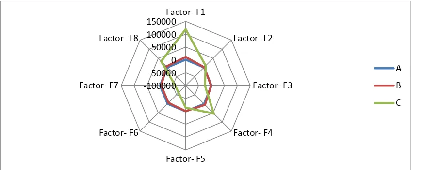
Graph 4.6.7 drawn below, indicate co-ordinate position of Model-A, Model-B and

Model-C. As shown by this graph, Model- A covers least or minimum area, Model-B

covers area at moderate or medium level whereas Model-C covers the maximum or

factors of these models. Graph 4.6.7 Simple Radar type graph indicating

co-ordinate position of models: - Graph 5.3 simple radar type indicates position of

[image:17.595.71.507.143.319.2]

models by drawing simple lines.

Table 4.6.7 Intensity of Positive Push and Negative Pull amongst models

Model Positive Push Negative Pull

A Minimum emphasis on F1,F2,F4 and F8 Minimum emphasis on F3,F5,F6 and F7

B More emphasis on F1,F2,F4 and F8 More emphasis on F3,F5,F6 and F7

C Highest emphasis on F1,F2,F4 and F8 Highest emphasis on F3,F5,F6 and F7

Graph 4.6.8 Filled Radar type graph indicating co-ordinate position of models: - Graph

4.6.8 filled radar type indicates position of models by highlighting areas covered by

respective model.

-100000 -50000 0 50000 100000 150000

Factor- F1

Factor- F2

Factor- F3

Factor- F4

Factor- F5 Factor- F6

Factor- F7 Factor- F8

A

B

C

-100000 -50000 0 50000 100000 150000

F1

F2

F3

F4

F5 F6

F7 F8

A

B

4.7 Testing of Hypothesis: -

Hypothesis Number 1:

-H1: Foreign banks (FBs) provide services to Indian companies at a very

competitive and concessional cost.

HO: Foreign banks (FBs) do not provide services to Indian companies at a very

competitive and concessional cost.

This hypothesis tested using statistical test, table supported with graph by comparing

A)Foreign banks’ cost of funds, B) Return on advances and C) Return on assets against State Bank of India (SBI) since in India SBI is the lead financial institution for

providing advances to manufacturing & trading.

Here we are comparing Foreign banks’cost of funds against SBI’s cost of funds since in India SBI is the lead financial institution for providing advances to manufacturing &

trading.

Table 4.7.1 FBs’ Cost of Funds - Comparison with State Bank of India

FBs (24) N

Average

SBI-Average

Year Cost of Funds Year Cost of Funds

2003-04 3.80 2003-04 5.74

2004-05 3.56 2004-05 4.90

2005-06 4.39 2005-06 4.88

2006-07 4.12 2006-07 4.55

2007-08 4.28 2007-08 5.64

2008-09 4.41 2008-09 5.72

2009-10 2.95 2009-10 5.14

2010-11 2.90 2010-11 4.67

2011-12 3.67 2011-12 5.35

2012-13 3.93 2012-13 5.63

Average= 3.80 Average= 5.22

Statistical Test: - Here x bar= 5.22, µo =3.80, σ= 0.43109, n=24

= (5.22-3.80)/ (0.43109/ (24^0.5)) = (1.42)/ (0.43109)/ 4.8989 =1.42/0.0879 =16.15

Distribution of test statistic is N (0, 1). So critical value for right tailed test and for 5%

level of significance is 1.645. Since, computed value > critical value at 5% level of

significance, we reject Ho at 5%level of significance in favor of H1 and conclude that

Foreign banks provide services to Indian companies at a very competitive and

concessional cost because FBs’cost of Funds is lower than SBI’s Cost of Funds.

Graph 4.7.1 FBs’ Cost of Funds- Comparison with State Bank of India (SBI)

From above table and graph it is observed that FBs cost of Funds is lower than SBI’s Cost of Funds during the observation period. Hence H1 is acceptable whereas HO is

rejected.

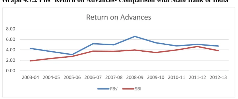
B) Here we are now, comparing FBs return on advances against SBI’s return on advances since in India SBI is the lead financial institution for providing advances to

manufacturing & trading 0

1 2 3 4 5 6 7

2003-04 2004-05 2005-06 2006-07 2007-08 2008-09 2009-10 2010-11 2011-12

Cost of Funds

Table 4.7.2 FBs’ Returns on Advances – Comparison with State Bank of India (SBI)

FBs 24(N) Average SBI-Average

Year Return on Advances Year Return on Advances

2003-04 4.27 2003-04 1.88

2004-05 3.66 2004-05 2.34

2005-06 3.08 2005-06 2.74

2006-07 5.16 2006-07 3.74

2007-08 4.96 2007-08 3.70

2008-09 6.57 2008-09 3.95

2009-10 5.35 2009-10 3.48

2010-11 4.74 2010-11 3.97

2011-12 5.04 2011-12 4.63

2012-13 4.72 2012-13 3.83

Average= 4.75 Average= 3.42

Statistical Test: - Here x bar= 4.75, µo =3.43, σ= 0. 0.90339, n=24

𝑍𝑐 =x bar − µo σ/√𝑛

= (4.75-3.43)/ (0.90339/ (24^0.5)) = (1.32)/ (0.90339)/ 4.8989 =1.32/0.1844 =7.15

Distribution of test statistic is N (0, 1). So critical value for right tailed test and for 5%

level of significance is 1.645. Since, computed value > critical value at 5% level of

significance, we reject Ho at 5%level of significance in favor of H1 and conclude that

FFIs provide services to Indian companies at a very competitive and concessional cost

because FBs’Return on Advances is higher than SBI’s Return on Advances.

Graph 4.7.2 FBs’ Return on Advances- Comparison with State Bank of India

0.00 2.00 4.00 6.00 8.00

2003-04 2004-05 2005-06 2006-07 2007-08 2008-09 2009-10 2010-11 2011-12 2012-13

Return on Advances

[image:20.595.104.519.580.752.2]

From above statistical tests, tables and graph it is observed that FBs’ return on advances

is higher than SBI’s return on advances during the observation period. Hence H1 is

acceptable whereas HO is rejected.

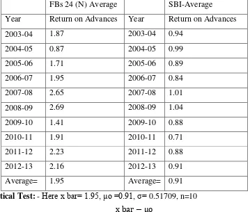
C) Here we are now, comparing FBs return on assets against SBI’s return on assets since in India SBI is the lead financial institution for providing advances to

[image:21.595.101.460.280.585.2]

manufacturing & trading.

Table 4.7.3 FBs’ Returns on Assets - Comparison with State Bank of India

FBs 24 (N) Average SBI-Average

Year Return on Advances Year Return on Advances

2003-04 1.87 2003-04 0.94

2004-05 0.87 2004-05 0.99

2005-06 1.71 2005-06 0.89

2006-07 1.95 2006-07 0.84

2007-08 2.65 2007-08 1.01

2008-09 2.69 2008-09 1.04

2009-10 1.41 2009-10 0.88

2010-11 1.91 2010-11 0.71

2011-12 2.23 2011-12 0.88

2012-13 2.16 2012-13 0.91

Average= 1.95 Average= 0.91

Statistical Test: - Here x bar= 1.95, µo =0.91, σ= 0.51709, n=10

𝑍𝑐 =x bar − µo σ/√𝑛

= (1.95-0.91)/ (0.51709/ (24^0.5)) = (1.04)/ (0.51709)/ 4.8989 =1.04/0.0.1055 = 9.85

Distribution of test statistic is N (0, 1). So critical value for right tailed test and for 5%

level of significance is 1.645. Since, computed value > critical value at 5% level of

significance, we reject Ho at 5%level of significance in favor of H1 and conclude that

FBs provide services to Indian companies at a very competitive and concessional cost

Graph 4.7.3 FBs’ Return on Assets- Comparison with State Bank of India (SBI)

From above statistical test, table and graph it is observed that FBs return on assets is

higher than SBI’s return on assets during the observation period. Hence H1 is

acceptable whereas HO is rejected.

Hypothesis Number 2: -

4.7.2 H1: Foreign Banks (FBs) provide advisory and promotional services to

Indian exporters and importers which results in enhancing Foreign Trade.

4.7.2.1 HO: Foreign Banks (FBs) provide advisory and promotional services to

Indian exporters and importers which do not result in enhancing Foreign Trade.

This hypothesis is tested using statistical test-regression analysis and table supported

with graph by comparing

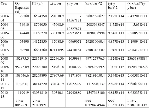
A) FBs’ Operating Expenses - Independent Variable B) FBIs’ Total Expenses - Independent Variable C) Foreign Trade (FT) - Dependent Variable

Statistical Test using Regression Analysis: - y= a + bx

x = Operating Expenses, independent variable, y = Foreign Trade (FT), dependent

variable,

0.00 0.50 1.00 1.50 2.00 2.50 3.00

2003-04 2004-05 2005-06 2006-07 2007-08 2008-09 2009-10 2010-11 2011-12 2012-13

Return on Assets

Table 4.7.4 India’s Foreign Trade and FBs’ Op. Expenses INR million

Year Op. Expenses (xi)

FT (yi) xi-x bar yi-y bar (xi-x bar)^2 (yi-y bar)^2

(x-x bar)*(y-y bar)

2003-04

29560 6524750 -51018.9 -14567171

2602928627 2.122E+14 7.43201E+11

2004-05

34910 8764050 -45668.9 -12327871

2085648847 1.52E+14 5.63E+11

2005-06

47440 11168270 -33138.9 -9923651 1098186998 9.848E+13 3.28859E+11

2006-07

63490 14122850 -17088.9 -6969071 292030660.4 4.857E+13 1.19094E+11

2007-08

89290 16681760 8711.095 -4410161 75883183.07 1.945E+13 -3.8417E+10

2008-09

102875.3 22151910 22296.36 1059989 497127776.3 1.124E+12 23633898884

2009-10

95775.09 22092700 15196.18 1000779 230923959.5 1.002E+12 15208020226

2010-11

108546.6 28263890 27967.69 7171969 782191650.4 5.144E+13 2.00583E+11

2011-12

113983.1 38114220 33404.19 17022299 1115840137 2.898E+14 5.68616E+11

2012-13

119919 43034810 39340.1 21942889 1547643106 4.815E+14 8.63235E+11

X bar= 80578.9 Y bar= 21091921 SSX= 10328404944 SSY= 1.355E+15 SSXY= 3.38701E+12

b=SSXY/SSX = 3.38701E+12 /10328404944=327.9315653 and a= y bar –b * x bar = 21091921 – (327.9315653*80578.9) = -5332443.807 Value b =327.9315653 is the change in the value of Y for a unit change in the value of X. The intercept is a

constant or the value of Y when X is zero. The values of a and b obtained using least

square method are called as least square estimates (LSE) of a and b. The values of a

and b obtained using least square method are called as least square estimates (LSE) of

a and b. Also the relation between the correlation coefficient for X and Y (r) and LSE

of b is given as under:-

𝒓 = 𝒃√(∫ (𝒙𝒊 − 𝒙𝒃𝒂𝒓)^𝟐)/(∫ 𝒚𝒊 − 𝒚𝒃𝒂𝒓)^𝟐)𝒊=𝒏 𝒊=𝟏

𝒊=𝒏

𝒊=𝟏

[image:23.595.76.567.151.511.2]

=327.9315653 * (10328404944 /1.355E+15 )^0.5 = 0.905378554 In the above model

Y=a + Bx + error , if b = 0 , then the model cannot be considered as a linear model.

Therefore, here we test Ho: b=0 against Ha: b≠0, the test statistic is 𝑻𝒄 = 𝒃𝒃𝒂𝒓

√𝑺𝑺𝒀/(𝒏−𝟐)𝑺𝑺𝑿

= (327.9315653) / ((1.355E+15)/(( 24-2)*( 10328404944 )))^0.5

= 4.246601837

At 5% level of significance and 22 d.f., the critical value using t distribution is 2.074

which is smaller than the computed value. Therefore, at 5% level of significance we

reject the null hypothesis and conclude that there is an evidence of linear relationship

between the independent variable-Op. Expenses and the dependent variable-FT

Graph 4.7.4 Operating Expenses Vs FT- Scattered Plot

Using SPSS the calculated value of ‘R’ is 0.905 and ‘R square’ is 0.819. Also the calculated value of standardised coefficient ‘Beta’ is 0.905. Since these values are closer to 1, it is concluded that there exists linear correlation between independent

variable ‘Operating Expenses’ and dependent variable ‘Foreign Trade’. This means that regression explains most of the variability in the dependent variable and the fitted model

is good.

0 5000000 10000000 15000000 20000000 25000000 30000000 35000000 40000000 45000000 50000000

0 20000 40000 60000 80000 100000 120000 140000

FT

-De

p

e

n

d

e

n

t

Vari

a

b

le

Op.Expences-Independent Variable

Table 4.7.5 India’s Foreign Trade and FBs’ Total Expenses INR million : - Statistical Test using Regression Analysis: - y= a + bx

x = Total Expenses, independent variable y = Foreign Trade (FT), dependent variable

Year Total Expenses (xi)

FT (yi) xi-x bar yi-y bar (xi-x bar)^2 (yi-y bar)^2 (x-x bar)*(y-y bar)

2003-04

64670 6524750 101342.089

-14567171

10270219003 2.12202E+14 1.47627E+12

2004-05

68030 8764050 -97982.089

-12327871

9600489765 1.51976E+14 1.20791E+12

2005-06

88920 11168270 -77092.089 -9923651 5943190186 9.84788E+13 7.65035E+11

2006-07

126360.8805 14122850

-39651.20852

-6969071 1572218337 4.8568E+13 2.76332E+11

2007-08

179156.2976 16681760 13144.20862 4410161 172770220.2 1.94495E+13

-57968076220

2008-09

214029.0414 22151910 48016.95243 1059989 2305627721 1.12358E+12 50897441391

2009-10

176456.7485 22092700 10444.65947 1000779 109090911.3 1.00156E+12 10452795855

2010-11

204374.008 28263890 38361.919 7171969 1471636829 5.14371E+13 2.7513E+11

2011-12

248835.414 38114220 82823.325 17022299 6859703164 2.89759E+14 1.40984E+12

2012-13

289288.5 43034810 123276.411 21942889 15197073509 4.8149E+14 2.70504E+12

X bar= 166012.089 Y bar= 21091921 SSX= 53502019646 SSY= 1.35549E+15 SSXY= 8.11894E+12 b=SSXY/SSX =8.11894E+12 /53502019646 = 151.7501592 and a= y bar –b * x bar

=21091921 - 151.7501592 *166012.089 = -4100439.935. The value b =151.7501592

is the change in the value of Y for a unit change in the value of X. The intercept is a

constant or the value of Y when X is zero. The values of a and b obtained using least

square method are called as least square estimates (LSE) of a and b. Also the relation

between the correlation coefficient for X and Y (r) and LSE of b is given as under:-

𝒓 = 𝒃√(∫ (𝒙𝒊 − 𝒙𝒃𝒂𝒓)^𝟐)/(∫ 𝒚𝒊 − 𝒚𝒃𝒂𝒓)^𝟐)𝒊=𝒏 𝒊=𝟏

𝒊=𝒏

𝒊=𝟏

= b√((SSX)/SSY)

[image:25.595.59.583.173.541.2]

In the above model Y=a + Bx + error , if b = 0 , then the model can not be considered

as a linear model. Therefore, here we test Ho: b=0 against Ha: b≠0, the test statistic is

𝑻𝒄 =_{√𝑺𝑺𝒀/(𝒏−𝟐)𝑺𝑺𝑿}𝒃𝒃𝒂𝒓

= (151.7501592) / ((1.35549E+15)/(( 24-2)*( 53502019646 )))^0.5

= 4.471749067 At 5% level of significance and 22 d.f., the critical value using t

distribution is 2.074 which is smaller than the computed value. Therefore, at 5% level

of significance we reject the null hypothesis and conclude that there is an evidence of

linear relationship between the independent variable- Total Expences and the

dependent variable-Foreign Trade FT

Graph 4.7.5 Total Expenses Vs FT- Scattered Plot

Graph 4.7.6 India’s Foreign Trade and FBs’ Yearly Expenses

Values for FT in INR million x 1000 whereas

Values for Op. Expenses & Total Expenses in INR million

0 5000000 10000000 15000000 20000000 25000000 30000000 35000000 40000000 45000000 50000000

0 50000 100000 150000 200000 250000 300000 350000

FT

-De

p

e

n

d

e

n

t

Vari

a

b

le

Total Expences-Independent Variable

Total Expenses Vs FT

Scattered Plot

0 10000 20000 30000 40000 50000

2003-04 2004-05 2005-06 2006-07 2007-08 2008-09 2009-10 2010-11 2011-12 2012-13

FT &FBs Yearly Expenses

Using SPSS the calculated value of ‘R’ is 0.953 and ‘R square’ is 0.909. Also the calculated value of standardised coefficient ‘Beta’ is 0.953. Since these values are closer to 1, it is concluded that there exists linear correlation between independent

variable ‘Total Expenses’ and dependent variable ‘Foreign Trade’. This means that regression explains most of the variability in the dependent variable and the fitted model

is good. Advisory and promotional services are part of operating expenses and total

expenses. From above statistical tests, tables and graphs it is observed that with increase

in operating expenses or total expenses there is increase in foreign trade. There exists a

linear relationship between an independent variable and a dependent variable. This

follows the equation y=a +bx. Hence H1 is acceptable whereas HO is rejected.

4.8 Conclusions: -Conclusionsemerging out on the basis of the research are as under:

4.8.1 Dependency: - The present study reveals that the three models of foreign banks

covering financing of foreign trade depends on the indicators covered under Factor F1,

Factor F2, Factor F4, Factor F8 involving variables in principle like M-EXDEM, log

(M-FT), Net Profit, FIN, Profit per Employee, EIR, Return on Advances, Profit per

Employee, Business per Employee which are termed as “PositivePush” having positive values.

4.8.2 Enhancing probability of financing: - So to enhance the probability of the foreign

banks for financing covering foreign trade, the other aspects should be taken care of

which are covered under Factor F3, Factor F5, Factor F6 and Factor F7.

4.8.3 It is concluded that there is no authentic declaration of self – defined model by any foreign banks operating in India.

4.8.4 Covering Basic Elements: - Although all 24 cases of foreign banks are covering

elements of basic business models like interest model, investment model, retail

financing model or profitability model etc., emphasis on these basic elements varies

from institution to institution. Hence, these foreign banks are grouped into three clusters

possessing totally different values for all eight number factors as indicated by the graph.

4.8.5 Least & Medium Values:-We can very well conclude that ‘Low End Also Ran

‘Model-A possesses least values for eight factors indicating that these foreign banks are carrying out minimum acceptable level of business including financing of foreign trade

as indicated by the values of factors whereas, ‘Progressive Medium End Economic’

4.8.6 Highest Level:-It is conclude that ‘High End Star ‘Model-C possesses highest level for eight factors indicating that these FFIs are carrying out excellent level of

business including financing of foreign trade as indicated by the values of eight factors.

4.8.7 Since, the contribution of foreign banks in overall credit allocation amounts to a

small figure of mere 5.75 percent it is concluded that the foreign banks are not

effectively using their available resources to counter the challenges posed by the other

financial institutions especially for the allocation of advances to manufacturing /trading.

4.8.8 Since, the contribution of foreign banks in overall investment allocation amounts

to a non-significant figure of mere 7.84 percent it is concluded that the foreign banks

are not taking full advantage of the buoyancy in economic growth and not expanding

financial activities in all segments including priority sector.

4.8.9 Based on the research findings it is concluded that the foreign banks are not

initiating efforts on adopting the new technologies in order to improve their customer

service levels and provide new delivery platforms to them, especially in the rural area

other than metro cities and urban area.

4.8.10On the basis of the study, we conclude that only Model-C possesses prominent

values for eight Factors considering involved positive push or negative pull for

financing of foreign trade for foreign banks during the observation period. This trend is

followed by Model-B and further by Model-A with drastic decrease in values for eight

Factors. Positive push effect of Factors indicates that the foreign banks maintain the

proper balance in financial/foreign trade variables and able to minimize the financial

burden on it, which directly enhances the profitability and foreign banks’ survival in stiff competition with grace. Thus, it is concluded that this research is helpful to the

BIBLIOGRAPHY

1 Amit R., Zott C.(2001) “Value Creation in E-Business”. Strategic Management Journal, 22(6/7), pp. 493.

2 Amit. R, Zott C. (2011) “The business model”Journal of management, 37(4), pp. 1019

3 A.Afuah (2004) “Business models: a strategic management approach”. Boston: McGraw-Hill/Irwin.

4 AYADI, R., ARBAK, E. and DE GROEN, W.P., 2011. BUSINESS MODELS IN

EUROPEAN BANKING: A PRE-AND POST-CRISIS SCREENING. Centre for

European Policy Studies: Centre for European Policy Studies.

5 AYADI, R., ARBAK, E. and DE GROEN, W.P., 2012. REGULATION OF

EUROPEAN BANKS AND BUSINESS MODELS: TOWARDS A NEW

PARADIGM? Centre for European Policy Studies: Centre for European Policy

Studies.

6 Adrian Blundell-Wignall and Caroline Roulet (2013) “Business models of banks, leverage and the distance-to-default” OECD Journal: Financial Market Trends Volume 2012/2

7 Adrian Blundell-Wignall, Paul Atkinson and Caroline Roulet (2014) “Bank

business models and the Basel system Complexity and interconnectedness” OECD

Journal: Financial Market Trends Volume: 2013, Issue: 2Pages 43–68

8 Benson Kunjukunju(2006) “Reforms in Banking Sector and Their Impact in Banking Services,” SAJOSPS, July-December 2006, pp.77-81

9 Christian Weller, (1999) “The Connection between More Multinational Banks and Less Real Credit in Transition Economies, Working Paper B8, Center for European

Integration Studies, Bonn, 1999”

10 Daniel Perez Liston and Lawrence McNeil-Prairie View A&M University (2013)

“The impact of trade finance on international trade: Does financial development matter?” Research in Business and Economics Journal -2013

11 GEORGE, G. and BOCK, A.J., (2011) The Business Model in Practice and its

Implications for Entrepreneurship Research. Entrepreneurship Theory and Practice,

35(1), pp. 83.

12 Gaurav Shard and Namratha Swamy 2014 “Impact of Foreign Banks on the Indian

13 Joydeep Bhattachrya (1994) “The Role of Foreign Banks in Developing Countries:

A Survey of the Evidence” Department of Economics, IOWA State University USA.

14 Kavaljit Singh (2006) “Entry of Foreign Banks in India and China: A Brief Note: was prepared by the author in March 2006 for discussion among activists and

campaigners associated with BankTrack.

15 Liston and Prairie (2013) “The impact of trade finance on international trade: Does

financial development matter?” Research in Business and Economics Journal -2013 16 Mandira Sarma and Anjali Prashad (2014) “Do Foreign Banks in India Indulge in

Cream Skimming?” Paper presented at the Annual International Studies Convention,

Jawaharlal Nehru University, and New Delhi. 10–12 December

17 Osterwalder A., Pigneur Y. et al. (2005) “Clarifying Business Models: Origins,

Present, and Future of the Concept”. Communications of the Association for

Information Systems, 16, pp.

18 Osterwalder A. and Y. Pigneur Y. (2010) “Business model generation.” Wiley - LA English.

19 Pinches GE et al. (1973) , Mingo KA, Caruthers JK (1973) The stability of

financial patterns in industrial organizations. J Finance 28(3):389–396

20 Pedrotti (2014) A Model for the Interest Margin of a Risk-neutral Bank. The Role

of the Bank Orientation, Journal of Entrepreneurial and Organizatinal Diversity ,

Publication date: 17 June 2014 | Vol.3, Issue 1 (2014) 167-180

21 Zott, C. and Amit, R., 2007. Business Model Design and the Performance of

Annexure 1:-Performance of Selected FFIs (which are operating consistently as

per profile of banks RBI during 2003-2013 (Values in INR Million))

Case

No

Name of FFI Business Advances Investment

1 AB Bank Limited 689.20 374.33 127.86

2 Abu Dhabi Commercial Bank Limited 7597.23 2021.00 4178.72

3 Antwerp Diamond Bank N.V. 5592.99 5399.19 1603.60

4 Bank of America NA 81790.70 42689.60 43381.06

5 Bank of Bahrain and Kuwait B.S.C. 8109.92 3580.48 2139.22

6 Bank of Ceylon 1717.35 586.24 408.86

7 Barclays Bank PLC 71792.28 51374.34 62156.03

8 BNP Paribas 71871.31 37821.67 26126.57

9 CTBC Bank Co.,Ltd. 2651.91 1637.60 401.47

10 Citibank N.A. 757288.94 345373.51 230106.83

11 DBS Bank Ltd. 70173.18 46119.61 67793.86

12 Deutsche Bank AG 243959.31 92063.16 69540.06

13 JPMorgan Chase Bank 35019.65 17135.28 70139.71

14 Krung Thai Bank Public Company Ltd. 917.28 114.91 282.61

15 Mashreq bank psc 618.35 355.27 739.81

16 Mizuho Bank Ltd. 19109.32 16092.98 3969.87

17 Shinhan Bank 8699.00 4332.52 1887.69

18 Societe Generale 15232.36 5664.84 14498.80

19 Sonali Bank Ltd. 353.18 89.93 56.04

20 Standard Chartered Bank 758245.01 369421.38 170748.12

21 State Bank of Mauritius Ltd. 7215.56 3994.01 2201.44

22 The Bank of Nova Scotia 66185.25 44802.37 19798.60

23 The Bank of Tokyo-Mitsubishi UFJ, Ltd. 42134.03 30815.38 13493.78

24 The Hong-Kong and Shanghai Banking Corpn.Ltd. 651544.67 241832.05 260351.51

Source: - https://www.rbi.org.in/Scripts/Publications.aspx?publication=Annual

Annexure 1 indicates that there are 24 number FFIs operating in India consistently

during the period 2003-04 to 2012-13, i.e. there is no break in allocation of advances,

investment or their business. Also there is substantial increase in their business,

Annexure 2:-List of Variables and Factor/Component Score Coefficient Matrix

F-1 F-2 F-3 F-4 F-5 F-6 F7 -F-8 M-EXDEM 0.079 0.003 -0.073 0.045 -0.044 -0.091 -0.1 -0.091 log(M-FT) -0.001 -0.061 -0.05 0.079 -0.019 -0.133 -0.184 -0.268 log(CTGDP) 0 0.035 0.045 -0.075 0.011 0.138 0.169 0.31 FIN 0.037 0.59 0.091 0.051 -0.075 -0.188 0.096 -0.706 EIR 0.051 0.147 0.023 0.806 -0.307 -0.028 -0.003 0.346 Advances 0.06 -0.037 -0.039 -0.025 0.054 0.017 -0.005 -0.038 Interest

Income 0.066 0.005 -0.017 0.024 -0.011 -0.028 -0.021 -0.03 Net Profit 0.074 0.011 -0.091 0.002 -0.008 -0.048 -0.122 -0.108 Net Worth 0.05 0.027 0.055 0.036 0.001 0 0.023 0.151 Deposits 0.072 0.009 -0.039 0.038 -0.047 -0.05 -0.066 -0.057 Investments 0.069 0.111 0.03 0.115 -0.155 -0.116 -0.068 0.045 Other

Income 0.061 -0.007 -0.008 0.013 0.008 -0.005 -0.03 0.009 Total

Income 0.065 0.002 -0.015 0.021 -0.006 -0.023 -0.024 -0.02 Interest

Expended 0.067 0.022 -0.007 0.017 -0.004 -0.026 0.021 -0.085 Operating

Expenses 0.057 -0.023 0.022 0.028 0 0.005 0.011 0.059 Total

Expenses 0.062 -0.002 0.007 0.022 -0.002 -0.008 0.014 -0.015 Cost of

Funds -0.025 0.002 0.104 0.006 0.223 0.073 0.982 -0.035 Return on

Advances -0.036 -0.152 0.437 0.051 0.127 0.001 0.224 0.746 Return on

Assets -0.011 0.007 -0.074 -0.194 0.961 0.071 0.215 0.083 CRAR 0.003 -0.139 -0.122 0.248 0.21 0.138 -0.038 -0.091 Net NPA 0.045 0.228 -0.104 -0.015 -0.124 -1.044 -0.11 0.181

Total Assets

6.10E-02 0.002 -0.008 0.026 0.008 -0.03 -0.024 0.05 Operating

Profit

7.10E-02

2.00E-02 -0.045 0.032 -0.033 -0.055 -0.085 -0.029 Profit per

Employee

-1.00E-02

3.71E-01 -0.02 0.12 0.131 -0.197 -0.066 0.511 Business per

Employee

-2.20E-02

-2.00E-02 -0.336 -0.065 -0.136 0.013 -0.31 0.489 No. of

Employees

6.70E-02

-2.70E-02 -0.003 -0.019 0.025 0.041 0.03 -0.213 No. of

Offices

6.30E-02

-5.10E-02 -0.028 -0.088 0.118 0.101 0.095 -0.361 Wages as %

of TE

-3.10E-02

1.38E-01 0.565 -0.076 -0.267 0.136 -0.118 -0.219

Extraction Method: Principal Component Analysis.

Annexure 3:- Mean or average values of variables for a period 2003-04 to 2012-13.

1 2 3 4 5 6 7 8 9

Case

Interest Net Net

No.

MEXDEM log(MFT) log(CTGDP)FIN EIR Advances Income Profit Worth

1

0.011302 8.520946 0.716171 0.728676 11.7043 0.075151 43.8134 47.93819 531.5655

2

1.993978 6.274364 4.005062 0.81605 29.5134 0.405733 596.4668 144.6181 1433.942

3

2.044258 6.263548 3.882866 1.252066 6.986132 1.083933 377.1952 86.5328 1819.67

4

437.2524 3.933352 7.378122 1.052328 14.47222 8.570286 6178.131 3443.636 25838.4

5

1.808457 6.316776 3.991011 0.705273 13.39842 0.718812 479.7283 111.3826 1295.653

6

0.056594 7.821317 1.812312 0.579443 22.19721 0.117693 130.1293 85.73568 876.3367

7

753.9447 3.696745 7.558103 1.581373 17.64512 10.31382 9065.067 -439.026 35880.32

8

233.3098 4.206151 7.049174 0.88976 12.99163 7.593009 4913.651 1366.48 13033.78

9

0.155231 7.383107 2.439222 0.768909 11.47449 0.328762 187.9065 13.712 910.3369

10

18764.13 2.300756 9.977276 0.759922 15.56539 69.33656 53758.74 16679.69 99661.99

11

738.2202 3.705898 7.539043 1.623319 18.09345 9.258889 8344.631 2310.356 13996.96

12

1511.579 3.394653 8.391434 0.662419 15.37398 18.48243 14153.77 5001.229 39262.5

13

283.7692 4.121119 6.821963 2.492172 31.29069 3.440048 5361.748 3264.549 24558.35

14

0.007668 8.6894 0.671873 0.433381 71.51781 0.02307 82.1844 21.0976 443.5653

15

0.062057 7.781292 1.408714 1.77097 36.58039 0.071324 129.9595 82.2996 839.7577

16

15.08425 5.39556 5.284455 1.049899 7.917961 3.230798 1274.236 594.851 13221.21

17

1.931007 6.2883 4.049939 0.71505 15.82302 0.869791 685.5371 213.9429 2814.713

18

19.39233 5.286454 5.295083 1.323737 25.75065 1.137264 1458.734 298.1882 4359.767

19

0.00119 9.498512 -0.55174 0.413322 15.96035 0.018055 14.3541 9.499031 62.4212

20

14893.19 2.401096 9.877483 0.712394 13.99471 74.16436 51699.46 18836.64 92940.9

21

2.075999 6.256857 4.000183 0.858625 14.86414 0.801832 593.6765 85.40633 2273.813

22

209.4332 4.253039 6.966492 0.976063 8.902914 8.994443 3988.717 1584.072 8600.663

23

98.17731 4.582073 6.44133 1.051624 9.293006 6.18644 2863.675 1060.98 16126.01

Annexure 3 continued: - Mean or average values of variables for a period 2003-04

to 2012-13.

10 11 12 13 14 15 16 17 18

Return

Case

Other Total Interest Operating Total Cost of on

No.

Deposits InvestmentsIncome Income Expended Expenses Expenses Funds Advances

1

417.1836 0.100436 94.0111 137.8245 5.2742 51.8309 57.1051 1.592846 6.354355

2

7750.156 3.282207 123.4759 668.2895 619.1629 200.8647 498.5562 5.725984 3.230653

3

629.8798 1.25956 108.4462 483.2839 162.062 96.7826 271.1048 2.224303 2.892833

4

41952.85 34.07395 3427.549 9605.212 2302.402 2203.741 4506.562 3.166396 4.490603

5

4782.346 1.680269 90.7858 569.6926 256.1434 149.5937 405.7836 4.464146 4.70348

6

951.2952 0.321147 57.6074 188.2314 42.8481 33.923 76.22146 4.18408 6.647047

7

45184.81 48.82088 2625.642 11689.79 4546.924 4413.386 8796.007 5.193408 9.205074

8

35091.98 20.52129 1626.03 5986.015 2189.788 2063.796 4247.156 5.077408 3.329056

9

995.5634 0.315342 29.0727 216.229 64.6503 89.2132 157.1371 4.340328 4.737434

10

447915.7 180.739 17177.3 70935.49 19982.92 21144.78 41128.27 3.317731 6.873367

11

59807.56 53.24915 1044.025 9388.656 4701.185 1731.285 6432.47 4.594502 2.830329

12

112327.7 54.62072 7744.555 21899.64 4553.562 8116.914 12665.88 3.233051 5.90056

13

43242.6 55.09172 2836.417 8204.067 2252.027 1219.237 3470.678 2.615328 2.294875

14

866.9246 0.221984 14.1611 96.314 28.7083 30.9674 59.3 3.157066 5.266961

15

955.5095 0.581091 114.1018 241.6044 70.6079 69.2621 137.5054 3.384267 3.34988

16

6288.849 3.118168 396.0624 1670.584 296.2555 348.1234 644.0441 3.490809 3.855291

17

5578.31 1.482705 93.8473 782.2434 278.2324 134.0562 412.228 3.425068 4.943309

18

9648.415 11.38818 271.6336 1730.336 851.7249 482.903 1334.35 4.239087 3.906913

19

294.5599 0.04402 48.3475 63.14486 9.0565 37.0362 45.39638 1.885575 8.149363

20

416442.7 134.1153 20082.57 71852.82 21533.57 19433.5 40966.16 3.978731 6.48731

21

3641.168 1.729137 75.862 670.1248 381.7894 83.5198 465.6713 7.224513 2.021624

22

32306.82 15.55095 1274.11 5262.895 2393.521 500.8424 2894.537 4.258191 2.034303

23

17542.37 10.59878 820.067 3683.498 1019.768 648.711 1668.142 2.739569 4.286336

Annexure 3 continued: - Mean or average values of variables for a period 2003-04

to 2012-13.

19

20

21

22

23

24

25

26

27

28

Return

Profit

Business

Wages

Case

on

Total

Operating Per

Per

No.of

No.of

as a

No.

Assets

CRAR

Net NPA Assets

Profit

Employee Employee Employee Offices

% of TE

1

4.704

61.474

3.313 1004.768 82.4107

1.576 24.7026

27.9

1 18.07216

2

1.039

43.026

5.98 10274.44 169.7357 1.09029 168.4531

45.1

2 12.11498

3

0.89

36.901

2.267 9474.317 257.1901

3.2758 256.5594

21.8

1 18.36223

4

2.797

18.058

0 148290.5 6094.65

9.1727 263.7559

310.1

5 25.01976

5

0.658

24.114

3.439 8819.033

192.91

0.41

89.12

91

2 16.09609

6

2.927

57.625

7.832 2316.229 131.009

2.2425 58.0186

29.6

1 14.29878

7

1.901

19.875

1.481 240573.3 3527.787

6.6371 101.7176

705.8

5 31.57544

8

1.26

13.386

0.093

121104 2951.904

3.02 216.5451

331.9

9.1 21.58325

9

-0.392

37.548

2.926 3049.052 59.0937 -0.3512 94.7111

28

1.1 19.39872

10

2.479

13.689

1.395 1138294 37331.23

3.0513 174.6354

4336.4

39.3 16.20449

11

1.012

24.428

0.488 180835.9 5230.27

3.0249 192.6776

364.2

6.4 17.18687

12

1.871

14.251

0.235

302167 10628.74

3.7534 164.8151

1480.2

11 26.88934

13

2.706

20.401

0.844 167094.7 6107.39 13.7328 219.0097

159.9

1 24.44333

14

1.788

91.214

0 1815.272 39.0304

1.9135 89.0565

10.3

1 13.40693

15

4.535

72.071

0 4663.985 120.098

5.3007 45.8039

13.5

1.7 26.32301

16

2.227

46.5

0.25 113444.4 1131.529

3.9013 170.619

112

1.7 23.23686

17

1.962

53.25

0.08 15428.12 411.0154

3.8496 183.9114

47.3

2 13.89535

18

1.276

32.079

0.137 27607.41 485.9805

2.5831 158.3406

96.2

2.1 19.39847

19

2.18

46.447

4.579 476.9954 17.72746

0.2133

9.5456

37

1.7 48.85536

20

2.465

11.219

1.105 1068690 35833.66

2.1989 107.8953

7027.6

89.2 19.22794

21

1.166

39.378

1.988 10555.3 195.3515

2.1

211.6

34.1

3 6.989311

22

1.609

15.07

1.36 97942.94 2747.365

6.5996 343.2845

192.8

5 7.167538

23

2.118

40.831

0.011 83137.66 2212.355

4.3942 229.4882

183.6

3.1 22.46892

Annexure-4 Case wise calculations of values of 8 number factors:- Case No Factor-1 Factor-2 Factor-3 Factor-4 Factor-5 Factor-6 Factor-7 Factor-8

1 153.19 16.65 -8.74 93.12 -7.61 -55.33 -66.94 101.85

2 1454.31 144.33 -397.18 698.33 -323.27 -758.98 -816.36 267.57

3 831.00 80.16 -110.63 373.25 -0.37 -353.76 -354.63 781.64

4 15896.68 1546.18 -2306.81 7191.02 -1152.21 -7557.46 -7119.14 7919.86

5 1098.70 106.91 -239.53 514.67 -181.21 -549.23 -564.50 327.67

6 304.73 43.83 -41.68 170.63 -34.55 -135.81 -143.32 197.56

7 22665.80 1947.68 -2124.05 10303.29 -492.44

-10379.32

-8549.24 13907.07

8 12253.56 1000.25 -2081.33 5505.55 -903.19 -5976.61 -5587.55 5420.26

9 355.66 46.53 -44.35 179.31 -39.49 -151.50 -158.28 255.81

10 126632.3

7

10035.12

-27215.16

57051.91

-14982.28 -64862.55 -63737.27 37029.63

11 18696.81 1514.12 -3803.40 8369.58 -1761.95 -9471.92 -9043.40 6467.22

12 34207.79 2868.54 -6118.46 15419.74 -3535.42

-16685.74

-16132.75

12517.40

13 16735.02 1598.96 -2524.03 7591.41 -1043.39 -8108.74 -7602.53 8649.79

14 221.58 35.98 -59.45 178.26 -43.80 -93.66 -128.57 156.14

15 45