Stochastic choice, systematic mistakes and preference estimation

(1)

Munich Personal RePEc Archive

Stochastic choice, systematic mistakes

and preference estimation

Breitmoser, Yves

28 July 2016

Online at

https://mpra.ub.uni-muenchen.de/72779/

(2)

Stochastic choice, systematic mistakes

and preference estimation

Yves Breitmoser

∗

Humboldt University Berlin

July 28, 2016

Abstract

Individual choice exhibits “presentation effects” such as default, ordering and round-number effects. Using existing models, presentation effects bias utility estimates, which suggests instability of preferences and obscures behavioral patterns. This pa-per derives a generalized model of stochastic choice by weakening logit’s axiomatic foundation. Weakening the axioms implies that focality of options is choice-relevant, alongside utility, which entails presentation effects. The model is tested on four well-known studies of dictator games exhibiting typical round-number patterns. The gen-eralized logit model captures the choice patterns reliably, substantially better than existing models: it robustly predicts and controls for the round-number effects, thus provides “clean” utility estimates that are stable and predictive across experiments.

JEL–Code:D03, C10, C90

Keywords: stochastic choice, systematic mistakes, axiomatic foundation, utility

esti-mation, dictator game

∗_{I thank Nick Netzer, Martin Pollrich, Sebastian Schweighofer-Kodritsch, Georg Weizsäcker and}

(3)

1 Introduction

Economic studies analyze individual choice in order to understand preferences, amongst others social, time and risk preferences. These analyses make for a large and important literature, as a reliable understanding of preferences is required as basis for the theoreti-cal analyses and counterfactual predictions underlying policy recommendations. Prefer-ences often appear to be unstable, however, as small details in presentation substantially affect choice patterns. Examples include default effects (McKenzie et al., 2006; Dinner et al., 2011), left-digit effects (Poltrock and Schwartz, 1984; Lacetera et al., 2012), round-number effects (Heitjan and Rubin, 1991; Manski and Molinari, 2010), and positioning effects (Dean, 1980; Miller and Krosnick, 1998; Feenberg et al., 2015). Absent a model of such presentation effects that would allow researchers to control for them, they induce bi-ased and incoherent utility estimates. Thus, presentation effects may be a major reason for the failure to reach a consensus on preference theories that has been plaguing behavioral analyses (see, e.g., the recent critique by Levine, 2012). Moreover, without a predictive model of how choice and welfare depend on presentation, the effects of "nudging" inter-ventions remain elusive.

The present paper shows that presentation effects can be modeled similarly to stochas-tic mistakes and in fact represent a generalization thereof. I axiomastochas-tically derive a model of stochastic choice with presentation effects by weakening the axioms underlying multi-nomial logit. Put briefly, in this generalized model two attributes of options affect choice, utility and focality, and focality captures the choice-relevant implications of presentation. I then apply this “focal choice adjusted logit” model (FOCAL) to data from controlled experiments to test the above intuition: First, do existing models indeed yield significantly biased estimates that suggest preference instability? Second, does the FOCAL model capture presentation effects to the point that utility estimates are coherent across stud-ies? Based on an analysis of predictive accuracy and robustness across experiments on generalized dictator games, both empirical questions will be answered in the affirmative: Existing models indicate preference instability even across simple dictator games, while controlling for focality factors out presentation effects and yields stable, even predictive estimates. This exercise showcases how the FOCAL model is able to both (i) facilitate the emergence of a consensus in behavioral modeling and (ii) reliably predict presentation effects, as envisaged by various "nudging" interventions.1

As point of departure, let us revisit the axiomatic foundation of logit (McFadden, 1974), as analyzed in Breitmoser (2016). Consider a decision maker (DM) with utility functionuwho choosesx∈Bwith probability Pr(x|u,B). If the choice probabilities satisfy positivity and independence of irrelevant alternatives (IIA), they are functions of choice

1_{The analysis of predictive adequacy relates the paper to the literature studying predictive adequacy in}

(4)

“propensities”vsuch that

Pr(x|u,B) = exp{v(x,y|u)}

∑x′∈Bexp{v(x′,y|u)}

with v(x,y|u) =log

_Pr

(x|u,B)

Pr(y|u,B)

for allx∈Bin relation to a benchmark optiony∈B. Formally,vrepresents the log-odds of the choice betweenxandy. Without further restrictions,vmay be any function ofu(x)

andu(y). McFadden (1974) assumes v(x,y|u) =u(x)−u(y)in Axiom 3 (“Irrelevance of Alternative Set Effect”). Givenv’s definition, this is equivalent to assuming

Pr(x|u,{x,y})

Pr(y|u,{x,y}) =exp{u(x)−u(y)} ⇔ Pr(x|u,{x,y}) =

exp{u(x)}

exp{u(x)}+exp{u(y)},

i.e. to assuming that binomial choice is logit. Thus, binomial logit is assumed by axiom and itself not independently founded. (IIA merely extends binomial logit to multinomial choice.) Breitmoser (2016) shows that logit is founded in axioms called “narrow bracket-ing” and “absence of systematic mistakes”. Dropping the latter axiom implies that choice probabilities take the generalized logit form

Pr(x|u,B) = exp{λ·u(x) +w(x)}

∑x′_∈_Bexp{λ·u(x′) +w(x′)}.

In general, that is, choice propensities are predicted to depend on two option attributes,

u(x) and w(x). By assumption, the former is DM’s utility, and the second component therefore induces systematic deviations from maximizing utility—i.e. it captures “system-atic mistakes”. Thus, the system“system-atic mistakes in choice are theoretically predicted, but had been unknowingly assumed away in logit. Sincew(x)is an attribute of optionxthat is

in-dependent of utility, it is intuitively interpreted asx’s focality—capturing a notion debated

at least since Schelling and relating intimately to the received understanding of systematic mistakes in choice. For example,w(x)may reflect that default options are relatively focal, that top-left or bottom-right positioning elevates focality, that labeling, coloring, or level of “roundness” affects focality, and so on, thus inducing deviations from utility maximization and capturing the various manifestations of presentation effects.

Building on this observation of Breitmoser (2016), note first that generalized logit offers a framework, but not yet an applicable model of choice. While w(x) intuitively relates to focality, the formal relation is indeterminate. If a focality index φ is given, physically or neuro-economically measured, assumed based on previous work, or to be estimated econometrically, then w(x) may be an arbitrary function of φ(x). Section 2 shows that an axiom capturing “relativity of focality” implies that the choice probabilities are uniquely represented by “focal choice adjusted logit” (FOCAL),

Pr(x|u,φ,B) = exp{λ·u(x) +κ·φ(x)}

∑x′_∈_Bexp{λ·u(x′) +κ·φ(x′)}.

(5)

[image:5.595.91.505.137.222.2]

Figure 1: Dictator choice across experiments

(a) AM02 Treatment 4

Treatment 4 (B=60, Transfer 1:2)

Tokens transfered

P

ercentage of choices

0 10 20 30 40 50 60

0 5 10 15 20 25 30

(b) HJ06 Treatment 6

Tokens transfered

P

0 20 40 60 80 100

0

5

10

15

20

(c) CHST07 Treatment 2

Tokens transfered

P

0 100 200 300 400 500 600

0 5 10 15 20 25 30

(d) FKM07 “Treatment” 7

Transfer 1:2

Budget share transfered

P

0.0 0.2 0.4 0.6 0.8 1.0

0

5

10

20

30

Note:Andreoni and Miller (2002, AM02) and Harrison and Johnson (2006, HJ06) analyze generalized dic-tator games with numerical choice entry and budgets up to 100 tokens; choices are predominantly multiples of 10. The difference between AM02 and HJ06 is that the Leontief choice is not generally a multiple of 10 in HJ06. Cappelen et al. (2007, CHST07) analyze dictator games with with numerical choice entry and budgets up to 1600 tokens; choices are predominantly multiples of 100. Fisman et al. (2007, FKM07) ana-lyze generalized dictator games with graphical user interface and budgets up to 100 tokens; choice exhibit no round-number effects. In FKM07, treatments as such are not defined, as budget sets and transfer rates are individually randomized; the plot above therefore shows the budget share transferred. Plots for all treatments of all experiments are provided as supplementary material.

applicable using existing methods—while being theoretically attractive: It is derived from comparably general axioms reflecting standard practice even in least-squares analyses, it captures a general intuition about choice debated at least since Schelling, and it is a formal representation of informal arguments often made in view of presentation effects.2

We do not know the focality index φ, however. This may suggest that controlling for focality might in general not improve robustness of estimates, as we would likely overspecify the focality index, in which case we risk misspecification, or underspecify it, in which case we risk overfitting. We need to specifyφ only up to linear transformation, though, which extends the range of appropriate specifications and largely resolves these concerns. For example, if focality is bimodal, either high or low as in default or positioning effects, the focal option may be assigned focality 1 and the other option focality 0 without any loss of adequacy. In other cases, the qualitative properties of focality are understood, as in ordering and round-number effects. Sinceφ needs to be defined only up to linear transformation, such a qualitative understanding seems sufficient to control for focality at least in substantial manner.3 _{To test this hypothesis, a case where focality is qualitatively}

understood but certainly not trivial will be analyzed in detail.

Specifically, I cross-analyze existing data from multiple influential experimental stud-ies exhibiting one of the most prominent presentation-related biases: round-number ef-fects. For a transparent analysis of utility in relation to focality, data sets on “generalized dictator games” are particularly suitable: there is consensus on the functional form of

util-2_{For example, if there is a default option, this option has relatively high focality}_φ₍_x₎_{, which by FOCAL}

induces the default effect. If options are ordered and say the first option is “focal” (i.e. has high relative focality), ordering effects result, and similarly other presentation effects are usually related to focality.

3_{The focality index} _φ_{may contain flexible parameterization to verify the qualitative understanding. If}

(6)

[image:6.595.79.524.161.231.2]

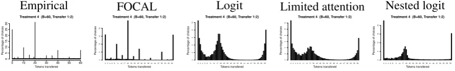
Figure 2: The adequacy of the choice models in capturing numerical choice: AM02 treat-ment 4, with budget 60 and transfer ratio 1 : 2. See Figure 3 for further plots

Empirical FOCAL Logit Limited attention Nested logit

Tokens transfered

P

0 10 20 30 40 50 60

0 5 10 15 20 25 30

0 2 4 6 81114172023262932353841444750535659

Tokens transfered

P

0

5

10

15

20

0 2 4 6 81114172023262932353841444750535659

Tokens transfered

P

0 2 4 6 8 10

0 2 4 6 81114172023262932353841444750535659

Tokens transfered

P

0 2 4 6 8 10 12

0 2 4 6 81114172023262932353841444750535659

Tokens transfered

P

0

5

10

15

20

Note: These plots depict the predicted choice distributions for AM02’s treatment 4 after fitting the model parameters to all data from AM02. The econometric methodology is standard and described in Section 4 and Appendix A; all models are described in Section 2. Besides FOCAL and logit, I consider more two benchmark models prominently discussed in the literature: Limited attention (Manzini and Mariotti, 2014; Echenique et al., 2014) and the cross-nested logit model allowing for similarity effects between proximate options (Ordered GEV, Small, 1987). More plots are provided below.

ities (CES), consensus on the nature of the presentation effects (round-number effects), and no additional influences due to e.g. risk or uncertainty. Further, the literature on gen-eralized dictator games is unusually rich, containing four extensive within-subject studies of dictator choice varying only presentation—including a graphical experiment without round-number effects (Fisman et al., 2007). This allows me to analyze reliability directly. Figure 1 provides an overview of the data sets, Section 3 describes them in detail.

To put the results into context, I relate FOCAL to three benchmark models capturing the main ideas in the existing literature: multinomial logit, limited attention, and nested logit (capturing similarity effects in choice). Section 4 analyzes the models’ adequacies to replicate the basic choice patterns in-sample. This clarifies how the models represent the observations internally and highlights their respective strengths and weaknesses. The differences are striking, see Figure 2. FOCAL reproduces the choice patterns rather ac-curately. Logit, despite having just one parameter less, fails in this respect and predicts choice patterns that do not resemble the observed ones: by ignoring the possibility of sys-tematic mistakes, logit assumes differences in choice probabilities indicate differences in utility, which is inadequate in the presence of round-number effects and yields instable preference estimates. Limited attention and nested logit are in-between FOCAL and logit, but only slightly improving on logit (detailed discussions follow).

(7)

even between simple dictator game experiments.

For its first test-case of social preference theory, FOCAL provides a rather positive perspective. If preferences were found to vary from application to application unpre-dictably, even across simple dictator game experiments, then differences to other games would be fairly uninformative and reliable application would be impossible. Having seen that these differences are likely due only to the inadequacy of prior choice models in capturing presentation effects and that the differences are resolved using adequate choice models suggests that a robust understanding of (social) preferences and the emergence of a consensus on their modeling are attainable. The results also indicate that experimental analyses need to analyze and control for (systematic) mistakes even if mistakes are not of explicit interest to the analyst. Systematic mistakes due to presentation are at the center of interest in behavioral welfare economics, and in this respect, FOCAL provides a first gen-eral model for econometric and theoretical analyses of nudging. The concluding Section 6 discusses these results and some implications for econometric and experimental analyses e.g. regarding graphical user interfaces following Fisman et al. (2007). The supplementary material contains robustness checks and some additional analysis.

2 Modeling choice with systematic mistakes

2.1 Utility and focality

The decision maker (DM) chooses an option x∈B from a finite budget B⊂X. Each option induces an outcome vector of dimensionalityn≥1 (say a payoff vector), denoted as π:X →_Rn_{. Further, each option is presented to DM in some way, as described by}

the injective functionl:X →L(not to be specified further) capturing the choice-relevant aspects of e.g. the default setting, positioning, coloring, or the number representing x.

Utility u:_Rn→_R maps outcome vectors to utilities, and focality φ:L→_R maps the presentation of options to their focality in the eyes of DM. Thus, utility and focality are orthogonal in the sense that changing the payoffs associated with options does not affect their focality and vice versa.4 For later reference, let me formalize this notion.

Definition 1 (Orthogonality). Utility u and focality φ are orthogonal if for any pair of decision taskshB,π,liandhB,π′,l′i,

π=π′ ⇒ u(π(x)) =u(π′(x))for allx∈B, (1)

l=l′ ⇒ φ(l(x)) =φ(l′(x))for allx∈B. (2)

Keeping orthogonality in mind, we may simplify notation by dropping references to outcome vectors and presentation, writingu(x) =u(π(x))andφ(x) =φ(l(x))for allx.

4_{Focality in this sense captures presentation effects that are independent of payoffs, but alternatively,}

(8)

Givenuandφ, the probability that DM choosesx∈Bfrom budgetB⊂X is denoted as Pr(x|u,φ,B). As point of departure, assume that budget B is derived from a “rich”

choice environmentX, that choice probabilities are positive and satisfy IIA, and that choice

exhibits a form of narrow bracketing (following Breitmoser, 2016).

Axiom 1(Richness). There existx,x′∈X such thatu(x)6=u(x′). For allx,x′∈X and all λ∈[0,1], there existsx′′∈X such thatu(x′′) =λu(x) + (1−λ)u(x′).

Axiom 2(Positivity). Pr(x|u,φ,B)>0 for allx∈B⊆X.

Axiom 3(Independence of Irrelevant Alternatives, IIA). For allB,B′⊆X,

Pr(x|u,φ,B)

Pr(y|u,φ,B) =

Pr(x|u,φ,B′)

Pr(y|u,φ,B′) for allx,y∈B∩B

′_.

Axiom 4(Narrow bracketing). For allr∈_Randx∈B⊆X, Pr(x|u,φ,B) =Pr(x|u+r,φ,B).

These axioms either reflect standard practice or are technically innocuous. Positivity and Richness are innocuous in that they are neither restrictive nor falsifiable (as probabil-ities can be arbitrarily low). Jointly with positivity and richness, IIA implies that choice probabilities are functions of choice propensitiesV or log-propensitiesv:=logV as in

Pr(x|u,φ,B) = V(x|u,φ)

∑x′∈BV(x′|u,φ)

or Pr(x|u,φ,B) = exp{v(x|u,φ)}

∑x′∈Bexp{v(x′|u,φ)}

.

IIA is innocuous in the sense that the relationship of propensitiesV (or,v) and utility or

focality is entirely unrestricted, i.e. v(x) may be an arbitrary function of u(x) and φ(x). IIA is considered restrictive in the presence of similarity effects, which may lead DM to partition the options into “nests” and then to first choose a nest and second an option from a nest (see e.g. the red-bus/blue-bus problem of Debreu, 1960). Such hierarchical choice violates IIA and can be modeled by “nested logit” as discussed below. In case similarity affects choice, FOCAL can be generalized straightforwardly to allow for nesting. Studies of numerical choice rarely relax IIA, however, noting that IIA is also obeyed in least squares analyses, which renders IIA in this context standard practice. I further discuss a model relaxing IIA below. Finally, narrow bracketing (Read et al., 1999) holds if DM considers the analyzed choice tasks in isolation, i.e. independently of his level of utility outside the experiment, which again is standard practice in experimental analyses.

Given orthogonality of utility and focality, these axioms imply that choice probabili-ties are generalized logit (Breitmoser, 2016), i.e. log-propensiprobabili-ties are linear inu.

Definition 2(Generalized logit). Consider a DM with utility functionuand focality func-tionφ. The choice probabilities are generalized logit if there existλ∈R andw:X →R

such that for all finiteB⊆X and allx∈B,

Pr(x|u,φ,B) = exp{λ·u(x) +w(x|φ)}

∑x′∈Bexp{λ·u(x′) +w(x′|φ)}

(9)

Briefly, let me clarify the main relations to the literature (for a detailed discussion, see Breitmoser, 2016). Generalized logit results if we assume choice satisfies positivity, IIA and narrow bracketing (besides richness of the environment). All three assumptions are equally satisfied in least squares analyses. Applications of least squares make additional assumptions on the irrelevance of utility differences between options and on the relevance of the options’ quadratic distances to the utility maximizer. These assumptions are not supported empirically, and they are made on top of logit’s assumptions. Thus, least squares makes strictly more assumptions than generalized logit, and hence is strictly less general, despite the seemingly specific functional form of generalized logit.

Generalized logit posits that utility and focality are additively separable. Their dis-tinction is not identified based on choice data alone, i.e. we cannot say ifwactually is part ofuor not. This reproduces a central result in behavioral welfare economics (K˝oszegi and

Rabin, 2008; Gul and Pesendorfer, 2008; Bernheim and Rangel, 2009). While it is not a concern in positive analyses of choice, it will be relevant in normative analyses of say nudging. Relatedly, if DM does not know the utilities associated with his options, but may learn about utilities by studying options, he has to decide which options to study and when to stop. If DM does so rationally, choice has a generalized logit representation similar to above (Matejka and McKay, 2015), but this generalization of logit captures similarity effects including the red-bus/blue-bus problem. Thus, both the above axiomatic analysis capturing presentation effects and the rational-inattention analysis capturing similarity ef-fects yield the same structure of choice propensities, and both reproduce the behavioral welfare result that true utilityuand biaswcannot be separated based on choice data alone.

This observation, that three fundamentally different approaches to choice analysis con-verge in the generalized logit model, appears to be rather reassuring.

2.2 Focal choice adjusted logit

The remainder of the paper uses these general observations of Breitmoser (2016) to de-velop and test a model of choice with systematic mistakes. As indicated, generalized logit predicts that options have two choice-relevant attributes, utilityu(x)and an attributew(x)

relating to focalityφ(x). So far, however,w(x)may be an arbitrary function ofφ(x). To fix ideas, let me define a focality indexφcapturing relative focality of round num-bers. Econometric models of rounding have been proposed in a growing literature starting with Heitjan and Rubin (1991) for consumption data and Manski and Molinari (2010) for subjective beliefs.5 This literature fairly consistently finds that 100,50,10,5,1,0.5,0.1, ...

exhibit decreasing levels of roundness (Battistin et al., 2003; Whynes et al., 2005; Covey and Smith, 2006). Thus, let us say that the focality index of a numberxis the level of the

highest number in this sequence that dividesx.

5_{This literature studies continuous-choice models to be applied in analyses of survey data. Utility}

(10)

Definition 3(Focality indexφ). Given the smallest notable differenceε>0, a potentially negative power of 10, define⌊x⌋εasxrounded down to the nearest multiple ofε. Further,

define an indexi:_Z→_Rsuch thati(0) =1,i(1) =5, andi(k) =10·i(k−2)for allk∈_Z. Then, for allx6=0 :φ(x) =max{k∈Z|i(k)divides⌊x⌋ε}, andφ(0) =φ(10).

This definition is very stylized, by assuming equidistant levels and by equating the level of “0” with that of 10. These assumptions can easily be relaxed, e.g. by introducing parameters to be estimated econometrically, but for transparency I restrict the degrees of freedom to a minimum. This freedom also concerns the definition of the base level of focality, i.e. the optionsxthat have zero focalityφ(x) =0. The above definition states that plain integers have zero focality, but there does not seem to be a rational justification for any such assumption, as focality inherently is relative. Therefore, I formally require that choice probabilities be invariant with respect to changes of the base level.

Axiom 5(Relativity). For allr∈Randx∈B⊆X, Pr(x|u,φ,B) =Pr(x|u,φ+r,B)

Relativity of focality is shown to imply that choice probabilities are linear in focality,

Pr(x|u,φ,B) = exp{λ·u(x) +κ·φ(x) +c(x)}

∑x′∈Bexp{λ·u(x′) +κ·φ(x′) +c(x′)}

. (4)

The constantc(x)is independent of both utilityuand focalityφand has a fairly intuitive explanation. Technically, we have not yet clarified that we captured all (known) factors of choice, and c(x) offers the possibility to include additional sources of say focality. As multiple sources of focality may as well be captured using a single focality index, this is technically not necessary, but it is logically consistent and illustrates how further extensions of logit can be achieved. The following axiom implies that choice is fully described by utility and focality.

Axiom 6 (Decision utility =true utility + focality). Given any B⊆X and any bijective

function f :B→B, Pr(f(x)|u,φ,B) =Pr x|u◦f,φ◦f,Bfor allx∈B.

Technically, Axiom 6 yieldsc(x) =const by requiring a form of permutation invari-ance. This implies that allc(x)cancel out and thus focal choice adjusted logit.

Definition 4(Focal choice adjusted logit, FOCAL). Consider a DM with utility function

uand focality functionφ. The choice probabilities are FOCAL if there existλ,κ∈Rsuch

that for all finiteB⊆X and allx∈B,

Pr(x|u,φ,B) = exp{λ·u(x) +κ·φ(x)}

∑x′_∈_Bexp{λ·u(x′) +κ·φ(x′)}.

(5)

The following proposition formally establishes the result.

(11)

satisfying richness (Axiom 1). Then,Pr(·)satisfies Axioms 3, 4, 5, and 6 if and only if the choice probabilities are FOCAL.

Proof. I proof that the axioms imply that choice probabilities are FOCAL; it is

straight-forward to verify that FOCAL satisfies the axioms. By orthogonality, Axioms 2–4 imply that choice probabilities satisfy (see Breitmoser, 2016)

Pr(x|u,φ,B) = exp{λ·u(x) +w(x|φ)}

∑x′∈Bexp{λ·u(x′) +w(x′|φ)}

= exp{λ·u(x)} ·exp{w(x|φ)}

∑x′∈Bexp{λ·u(x′)} ·exp{w(x′|φ)}

. (6)

Hence, there exists a function f :R→Rsuch that

Pr(x|u,φ,B) = exp{λ·u(x)} · f(φ(x))

∑x′_∈_Bexp{λ·u(x′)} · f(φ(x′)),

(7)

and by Axiom 5, for allr∈_R,

Pr(x|u,φ,B) = exp{λ·u(x)} · f(φ(x) +r)

∑x′∈Bexp{λ·u(x′)} · f(φ(x′) +r)

. (8)

The probabilities are invariant inronly if there exists a functiong:_R→Rsuch that

Pr(x|u,φ,B) = exp{λ·u(x)} · f(φ(x))·g(r)

∑x′_∈_Bexp{λ·u(x′)} · f(φ(x′))·g(r),

(9)

i.e. f(y+r) = f(y)·g(r) for all r, which implies f′(y) = f(y)·g′(0) and thus f(y) =

exp{a·y+b}for somea,b∈R. Hence, there existκ∈Randw:X→Rsuch that

Pr(x|u,φ,B) = exp{λ·u(x)} ·exp{κ·φ(x) +c(x)}

∑x′∈Bexp{λ·u(x′)} ·exp{κ·φ(x′) +c(x′)}

. (10)

Finally, by Axiom 6 this implies that the choice probabilities are FOCAL. For contradic-tion, assume the opposite, i.e. Eq. (10) and Axiom 6 are satisfied, but choice probabilities are not FOCAL, i.e. c(x)6= const. Fix x,y∈X such that c(x)6=c(y), B⊆X such that x,y∈B, and a bijection f :B→Bsuch that f(y) =xand f(x) =y. Thus,

Pr(x|u,φ,B)

Pr(y|u,φ,B) =

Pr(f(y)|u,φ,B)

Pr(f(x)|u,φ,B), (11)

and by Axiom 6

exp{λ·u(x) +κ·φ(x) +c(x)}

exp{λ·u(y) +κ·φ(y) +c(y)} =

exp{λ·u(f(y)) +κ·φ(f(y)) +c(y)}

exp{λ·u(f(x)) +κ·φ(f(x)) +c(x)}, (12)

(12)

2.3 Research hypotheses and benchmark models

FOCAL generalizes logit through capturing focality and by design, it thus appears more adequate than logit to analyze choice with presentation effects. For later reference, by logit, a DM with utilityuchoosesxwith probability

Logit: Pr(x|u,φ,B) = exp{λ·u(x)}

∑x′∈Bexp{λ·u(x′)}

. (13)

While the theoretical adequacy of FOCAL to capture effects relating to focality is imme-diate, it is unclear whether FOCAL improves on logit given the specific patterns in actual data. Further, it is unclear whether any such improvement implies that utility estimates are significantly more reliable given the comparably small size of typical (experimental) data sets. This yields the research hypotheses to be analyzed in Sections 4 and 5, respectively.

Hypothesis 1(Model adequacy). FOCAL captures choice with presentation effects signif-icantly more accurately than logit.

Hypothesis 2 (Reliability and consistency). FOCAL’s estimates are significantly more reliable across “similar tasks” than logit’s estimates.

These hypotheses are analyzed using data sets introduced in Section 3. The econo-metric analysis also allows me to clarify the relation to two other prominent models in the existing literature that intuitively apply to numerical choice and round-number effects.

Limited attention Round-number effects can be interpreted two ways: subjects either focus on some options or neglect other options. Masatlioglu et al. (2012) generalize re-vealed preference to account for DMs not considering all their options, Manzini and Mari-otti (2014) generalize this idea to stochastic choice, and Echenique et al. (2014) generalize the model further by allowing for a weak “perception ordering”: first all options at the highest perception level are considered, second the options at the next-highest level, and so on. This Perception Adjusted Luce Model (PALM) straightforwardly applies to focality effects, first the most focal options are considered, next the second layer, and so on, and hence it constitutes a natural benchmark for FOCAL. Formally, DM with utilityu, focality

φ, precisionλ, and choice biasκ∈[0,1], choosesx∈Bwith

PALM: Pr(x|u,φ,B) =µ(x,X)·

_∏

k>φ(x)

1−κ·

_∑

x′∈X:φ(x′)=k

µ(x′,X)

(14)

whereµ(x,X) =Logit(x) =exp{λu(x)}/∑x′∈Xexp{λu(x′)}. The focality indexφ used

(13)

Similarity/Nested logit Choice violates IIA in the presence of “similarity” effects, and intuitively proximate numbers are more similar than distant numbers. Such similarity ef-fects can be expressed by nested logit (McFadden, 1976) where DM first chooses a “nest” of options and secondly makes his final choice from this nest. Small (1987) introduces a cross-nested logit model (with overlapping nests) for choice from ordered sets, called

Ordered GEV,6which intuitively captures possible similarity effects in numerical choice.

Here, DM first makes a tentative choicey∈Band then reconsiders the neighborhood ofy

to make the final choicex∈[y−w,y+w]. To clarify the relevance of nesting and similarity effects, I include Ordered GEV as benchmark model. Formally, DM with utilityu,

preci-sionλ, degree of correlationκ, bandwidth parameterM<|X|, and options represented by their integer rankss=1,2, . . ., the choice probabilities are

OGEV: Pr(s) =

s+M

∑

r=s

wr−sexp

λu(s)/κ

exp{Ir}

· exp{κIr}

∑B_t₌+₀Mexp{κIt}

with Ir =ln

∑

s′∈Br

w_r₋_s′expλu(s′|α,β)/κ . (15)

3 Testing FOCAL: Preliminary remarks

The data selected for the analysis of the research hypotheses are from studies on general-ized dictator games.

Definition 5(Generalized dictator game). DM chooses an optionx∈ {0,1, . . . ,B}. Given

x, the dictator’s payoff isπ1(x) =τ1·(B−x)and the recipient’s payoff isπ2=τ2·x.

The data sets chosen satisfy the following requirements. First, there is consensus on the subjects’ true utilitiesu, there are unambiguous presentation effects, and the choice

task does not involve risk or (strategic) uncertainty. This enables an unconfounded analysis of focality and utility. Second, the data sets are from controlled experiments, which gives us perfect information of the choice environment, and they are from experiments run to estimate utility, so we avoid re-analyzing experiments out-of-context. Third, the data sets are representative for literally hundreds of experimental analyses (Engel, 2011), and in all cases, dictator games are analyzed to understand altruism. Thus, analyzing reliability of utility estimates is also relevant in the wider context. Finally, the data sets contain multiple observations per subject, which allows us to disentangle preferences, precision, and choice bias (i.e. to estimate FOCAL) while allowing for subject heterogeneity, and there exist even four such experiments, examining essentially equivalent choice tasks varying only presentation. This allows us to study reliability of counterfactual predictions.

Table 1 provides an overview of the data sets and Figure 1 above provides selected histograms of observed choices. In conjunction, these studies provide a fairly

comprehen-6_{All cross-nested logit models are compatible with random utility if utility perturbations have a}

(14)

[image:14.595.72.526.136.236.2]

Table 1: The data sets

#Treatments #Options #Observations Transfer ratios

“Numerical” dictator games

AM02(Andreoni and Miller, 2002) 8 41–101 176×8 3 : 1,. . . ,1 : 3 HJ06(Harrison and Johnson, 2006) 10 41–101 57×10 1 : 1,. . . ,1 : 4 CHST07(Cappelen et al., 2007) 6 401–1601 96×2 1:1

“Graphical” dictator games

FKM07(Fisman et al., 2007) 50 500–1000 76×50 4 : 1,. . . ,1 : 3

Table 2: Distribution of choices across “round” numbers

Percentage of choices with greatest factor . . .

Treat 0 1000 500 250 100 50 25 10 5 2.5 1 0.5 other

AM02 39 1 9 7 33 6 0 4

HJ06 22 3 4 7 39 14 0 10

FKM07 25 0 0 0 0 2 1 4 5 63

CHST07 30 0 5 1 62 1 0 0 0 0 0

Note:For each experiment, these percentages are pooled (and averaged) across treatments. The numbers do not always add up to exactly 100 due to rounding errors.

sive picture of dictator choice. Fisman et al. (2007, FKM07) use a graphical user interface which reliably prevents round-number effects (see Figure 1), while all other studies require subjects to enter numbers directly and thus reproduce the prevalent round-number patterns. Between those, Cappelen et al. (2007, CHST07) allow for budgets up toB=1600, and subjects primarily choose multiples of 100, while Andreoni and Miller (2002, AM02) and Harrison and Johnson (2006, HJ06) allow for budgets up toB=100 and choices mainly are multiples of 10. In AM02, the Leontief (payoff-equalizing) choice is generally a mul-tiple of 10 or 25, but in HJ06, it is often a plain integer. The latter drastically affects the relative frequency of the Leontief choice, see Figure 1b: the Leontief choice is frequent if and only if it is a round number. Thus we may drastically under- or overstate precision and inference on utility estimates if we do not control for focality.7

Regarding utility, following Andreoni and Miller (2002) and Fisman et al. (2007), analyses of dictator games mostly use utility functions exhibiting constant elasticity of substitution (CES) between dictator incomeπ1and recipient incomeπ2, i.e.

ui(πi,πj) = (1−α)·(1+πi)β+α·(1+πj)β

1/β

. (16)

Here, α represents the degree of altruism andβ represents the degree of efficiency

con-7_{The intuition is simple. Assume the Leontief choice is to transfer 10 out of 20. Without controlling for}

[image:14.595.86.514.282.370.2]

(15)

cerns. Subjects are efficiency concerned withβ=1 and equity concerned withβ→ −∞. Finally, regarding the round-number effects, Table 2 provides a detailed overview of the numbers chosen. In the experiments with numerical choice, subjects rarely choose plain integers. Mostly, they choose multiples of 10 and 100, as described above. In addi-tion, subjects tend to choose multiples of 5 and 50 reasonably regularly, while multiples of 2.5 and 25 are chosen a little less frequently. In this sense, the numbers chosen in numerical DG experiments do not differ substantially from those observed in survey re-sponses, i.e. there is no indication that using the focality index reflecting the patterns in survey responses, introduced in Definition 3, would be inadequate. There may be room for improvement, but then, the adequacy of FOCAL would only be underestimated.

4 Assessing model adequacy

The present section analyzes how the models reproduce the choice patterns in-sample. This “descriptive adequacy” identifies strengths and weaknesses of the models, but po-tentially involves overfitting. Overfitting will be verified in the next section by analyzing reliability of estimates across experiments (“predictive adequacy”).

The basic picture Figure 3 provides plots of the model fits in-sample. The underlying econometric model is simple and transparent: utilities exhibit CES, Eq. (16), preferences are heterogeneous between subjects (random parameters), error variance and choice bias are identical across subjects, and parameters are estimated by maximum likelihood.8 _This

specification is leaned on the well-known “mixed effects” regression models; the main analysis will use a specification allowing for heterogeneous error variance and choice bias. The figure contains a superset of the treatments already presented in Figure 1, skipping FKM07 where all models fit similarly due to the absence of round-number effects.

The differences between models are largely in line with the intuition. To begin with, logit interprets differences in choice probabilities to indicate differences in utilities, and utilities are continuous by assumption. Thus logit does not comprehend the mass points at round numbers, yielding a “blurry” representation of behavior. The contrast to FOCAL is striking: by adding just one parameter to separate utility and focality, FOCAL repro-duces the general shape of choice distributions. Parameters are fitted to all treatments per experiment, and thus there is some noise left in each treatment, but the overall accuracy is encouraging. Limited attention (PALM) and nested logit (OGEV) similarly generalize logit by adding one parameter, but without much of an effect. OGEV captures spikes at utility maximizers, most prominently zero transfers and Leontief transfers, but this mis-represents that spikes actually relate to round numbers. Limited attention, improves on

8_{Such mixed logit models are standard practice in analyses of consumer demand since Berry et al. (1995),}

(16)

Figure 3: The precision of the choice models in capturing numerical choice

Empirical FOCAL Logit

Limited attention (PALM)

Nested logit (OGEV)

AM02 #3

B=60,r=2 : 1

Tokens transfered

P

0 10 20 30 40 50 60

0 10 20 30 40 50

0 2 4 6 81114172023262932353841444750535659

Treatment 3 (B=60, Transfer 1:0.5)

Tokens transfered

P

0

10

20

30

0 2 4 6 81114172023262932353841444750535659

Tokens transfered

P

0 5 10 15 20 25

0 2 4 6 81114172023262932353841444750535659

Tokens transfered

P

0 5 10 15 20 25

0 2 4 6 81114172023262932353841444750535659

Tokens transfered

P

0 10 20 30 40 AM02 #4

B=60,r=1 : 2

Tokens transfered

P

0 10 20 30 40 50 60

0 5 10 15 20 25 30

0 2 4 6 81114172023262932353841444750535659

Tokens transfered

P

0

5

10

15

20

0 2 4 6 81114172023262932353841444750535659

Tokens transfered

P

0 2 4 6 8 10

0 2 4 6 81114172023262932353841444750535659

Tokens transfered

P

0 2 4 6 8 10 12

0 2 4 6 81114172023262932353841444750535659

Tokens transfered

P

0 5 10 15 20 AM02 #7

B=60,r=1 : 1

Tokens transfered

P

0 10 20 30 40 50 60

0

10

20

30

40

0 2 4 6 81114172023262932353841444750535659

Tokens transfered

P

0 5 10 15 20 25 30

0 2 4 6 81114172023262932353841444750535659

Tokens transfered

P

0 2 4 6 8 10 12 14

0 2 4 6 81114172023262932353841444750535659

Tokens transfered

P

0

5

10

15

0 2 4 6 81114172023262932353841444750535659

Tokens transfered

P

0 5 10 15 20 25 30 HJ06 #2

B=40,r=2 : 1

Tokens transfered

P

0 10 20 30 40

0

5

10

20

30

0246810121416182022242628303234363840

Tokens transfered

P

0 5 10 15 20 25 30

0246810121416182022242628303234363840

Tokens transfered

P

0 1 2 3 4 5 6

0246810121416182022242628303234363840

Tokens transfered

P

0 1 2 3 4 5 6 7

0246810121416182022242628303234363840

Tokens transfered

P

0 2 4 6 8 10 12 14 HJ06 #4

B=60,r=1 : 2

Tokens transfered

P

0 10 20 30 40 50 60

0 5 10 15 20 25

0 2 4 6 81114172023262932353841444750535659

Tokens transfered

P

0 5 10 15 20 25

0 2 4 6 81114172023262932353841444750535659

Tokens transfered

P

0 1 2 3 4 5 6 7

0 2 4 6 81114172023262932353841444750535659

Tokens transfered

P

0

2

4

6

8

0 2 4 6 81114172023262932353841444750535659

Tokens transfered

P

0 2 4 6 8 10 HJ06 #5

B=40,r=1 : 1

Tokens transfered

P

0 10 20 30 40

0

10

20

30

40

0246810121416182022242628303234363840

Tokens transfered

P

0 5 10 15 20 25

0246810121416182022242628303234363840

Tokens transfered

P

0

5

10

15

0246810121416182022242628303234363840

Tokens transfered

P

0

5

10

15

0246810121416182022242628303234363840

Tokens transfered

P

0 5 10 15 20 HJ06 #6

B=100,r=1 : 2

Tokens transfered

P

0 20 40 60 80 100

0

5

10

15

20

048 121722273237424752576267727782879297

Tokens transfered

P

0

5

10

15

048 121722273237424752576267727782879297

Tokens transfered

P

0 1 2 3 4 5

048 121722273237424752576267727782879297

Tokens transfered

P

0 1 2 3 4 5

048 121722273237424752576267727782879297

Tokens transfered

P

0

2

4

6

CHST07 #2

B=600,r=1 : 1

Tokens transfered

P

0 100 200 300 400 500 600

0 5 10 15 20 25 30

0 24 52 80 112 148 184 220 256 292 328 364 400 436 472 508 544 580

Tokens transfered

P

0 5 10 15 20 25

0 24 52 80 112 148 184 220 256 292 328 364 400 436 472 508 544 580

Tokens transfered

P

0 1 2 3 4 5

0 24 52 80 112 148 184 220 256 292 328 364 400 436 472 508 544 580

Tokens transfered

P

0 1 2 3 4 5

0 24 52 80 112 148 184 220 256 292 328 364 400 436 472 508 544 580

Tokens transfered

P

0 2 4 6 8 10 12 CHST07 #3

B=800,r=1 : 1

Tokens transfered

P

0 200 400 600 800

0 5 10 15 20 25 30

0 32 69 111 159 207 255 303 351 399 447 495 543 591 639 687 735 783

Tokens transfered

P

0 5 10 15 20 25

0 32 69 111 159 207 255 303 351 399 447 495 543 591 639 687 735 783

Tokens transfered

P

0 1 2 3 4 5

0 32 69 111 159 207 255 303 351 399 447 495 543 591 639 687 735 783

Tokens transfered

P

0 1 2 3 4 5

0 32 69 111 159 207 255 303 351 399 447 495 543 591 639 687 735 783

Tokens transfered

P

0 2 4 6 8 10 12

(17)

logit in the “right” direction, being based on the focality indexφ (see Definition 3) cap-turing “roundness” of numbers, but the effect is hardly visible. Round-number effects are much stronger than limited attention admits, which will be discussed below. This shows that the focality index itself is not capturing behavior, suggesting that FOCAL’s apparent adequacy stems from its separation of utility and focality in choice propensities.

Econometric analysis Table 3 provides the information on the quantitative differences between the models. As indicated, all models are used exactly as defined in Section 2, equipped with CES utilities and estimated by maximum likelihood. All parameters

(α,β,λ,κ)are allowed to be heterogeneous across subjects9 and the incomes in the CES utility function are the experimental tokens earned by the subjects.10 Likelihoods are com-puted by numerical integration using quasi-random numbers (Train, 2003) and maximized in a three-step approach, first using a gradient-free approach (NEWUOA, Powell, 2006), secondly using a Newton-Raphson method to ensure convergence, and finally using exten-sive cross-testing of estimates across data sets and models to ensure that global maxima are found. Appendix A provides the standard procedural details.

Table 3 reports both the Bayes information criterion (BIC) and the pseudo-R2. The former quantifies the model adequacy, the latter clarifies how much of the observed vari-ance is explained. This relates the model to the benchmarksclairvoyance, i.e. correctly

predicting the observed choice distributions, andnaivete, i.e. uniform randomization.11 In addition, relation signs indicate significance of differences, evaluated in likelihood ratio tests robust to both misspecified and arbitrarily nested models (Schennach and Wilhelm, 2014). I distinguish two levels of significance, namely the conventional level of 0.05, and the level of 0.005. The latter roughly implements the Bonferroni correction given the si-multaneous tests of four models on four data sets. I will focus on the latter level, but the distinction does not affect the main results (as Table 3 indicates). Finally, I pool the results for AM02 and HJ06 due to their similarity, both entailing numerical choice from up to

B=100 with 8 or 10 observations per subject. This way, Table 6 presents the results by type of data set: numerical choice with many observations per subject (“large numerical”), with few observations per subject (“small numerical”), and graphical choice (“graphical”). The results in Table 3 confirm Figure 3. In numerical DGs, the models can be parti-tioned into three equivalence classes, with logit and FOCAL as the extremes, and PALM and OGEV in-between, but improving only slightly on logit. In large numerical

exper-9_α_{is truncated normal on}_[₋_0.5,_0.5_]_,_β_{is normal,}_λ_and_κ_{are log-normal.}

10_{The supplement provides extensive robustness checks for both assumptions. Allowing for subject}

het-erogeneity in all dimensions allows for slightly more robust fit for all models, without obstructing identifi-cation. The token-based utility function used here fits best assuming the status quo model logit. The main alternative to the latter assumption is contextual utility (Wilcox, 2011), which tends to fit best for FOCAL and PALM, but these tendencies are overall minor and therefore not discussed here. The main results are comparably strong and perfectly robust to changing these assumptions, as shown in the supplement.

11_{Given a model’s log-likelihood, the BIC is defined as}_BIC₍_d_{) =}_|_ll₍_d₎_|₊_log₍_#_obs₎_·_#_par_{/2 (Schwarz,}

1978) and given the log-likelihoods of the “clairvoyant” model and the naive model, denoted asllmaxand

(18)

[image:18.595.67.536.167.345.2]

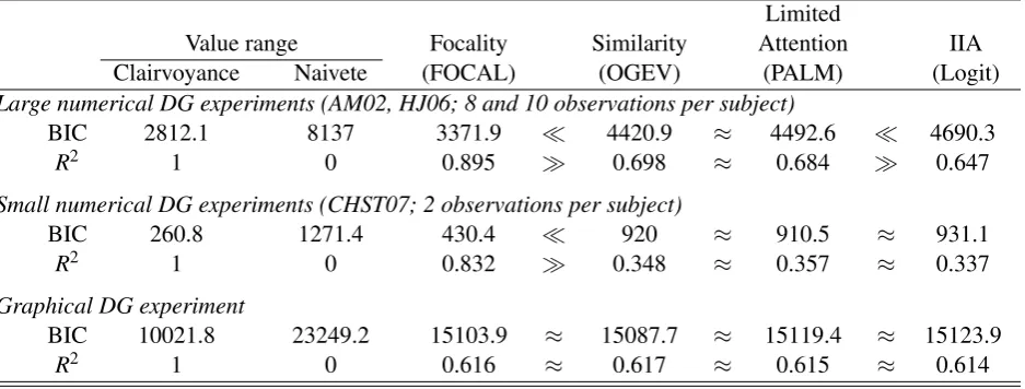
Table 3: Precision of the choice models in-sample (BIC: less is better;R2: more is better)

Limited

Value range Focality Similarity Attention IIA Clairvoyance Naivete (FOCAL) (OGEV) (PALM) (Logit)

Large numerical DG experiments (AM02, HJ06; 8 and 10 observations per subject)

BIC 2812.1 8137 3371.9 ≪ 4420.9 ≈ 4492.6 ≪ 4690.3

R2 1 0 0.895 ≫ 0.698 ≈ 0.684 ≫ 0.647

Small numerical DG experiments (CHST07; 2 observations per subject)

BIC 260.8 1271.4 430.4 ≪ 920 ≈ 910.5 ≈ 931.1

R2 1 0 0.832 ≫ 0.348 ≈ 0.357 ≈ 0.337

Graphical DG experiment

BIC 10021.8 23249.2 15103.9 ≈ 15087.7 ≈ 15119.4 ≈ 15123.9

R2 1 0 0.616 ≈ 0.617 ≈ 0.615 ≈ 0.614

Content: For each choice model (Logit, OGEV, PALM, and FOCAL), the descriptive accuracy (BIC and

pseudo-R2in-sample) is reported for data from the three groups of experiments. Significance of differences

is (following Schennach and Wilhelm, 2014) is denoted as follows: ≈indicates p-values above 0.05,>, < indicatep-values between 0.005 and 0.05, and≫,≪indicatep-values below 0.005.

iments, FOCAL’s adequacy (pseudo-R2) is 89%, logit is around 65%, and PALM and OGEV are around 69%. All differences are statistically significant and easily visible (see Figure 3). In the small numerical experiment, FOCAL’s adequacy is 83% and the other models are around 35%. In the graphical experiment, all models are around 62% adequacy. Aside from the high statistical significance, two observations stand out. First, FOCAL at-tains a substantially higher pseudo-R2 in numerical DGs than in graphical ones. This is

intuitive if a model captures round-number effects, as choices cover relatively few options in numerical DGs and thus indeed are more predictable than in graphical DGs. The other models are equally adequate in the (large) experiments with and without round-number effects, confirming the optical impression that they do not comprehend round-number ef-fects. Second, FOCAL’s adequacy is largely similar in the large and small numerical experiments, being 89% and 83%, respectively. These experiments differ in the relative strength of round-number effects: CHST07 implements the largest number of options, up toB=1600, but the smallest number of different options actually gets chosen by the sub-jects (see also the discussion of entropy following shortly). In this sense, the round-number effects are strongest in CHST07, and the observation that FOCAL’s adequacy is similar indicates that it is robustly adequate. In turn, the adequacy of the other models drops sub-stantially in CHST07, to around 35%: these models do not capture round-number effects, and thus, the stronger the round-number effects, the lower their adequacy.

(19)

Since OGEV fits only slightly better than logit, similarity effects appear to be of minor relevance in numerical choice. As for limited attention (PALM), the observation that it barely improves upon logit in the present context appears to relate to its axiom “Hazard Rate IIA” (Echenique et al., 2014), which is an implication of “I-Asymmetry” and “I-Independence” in Manzini and Mariotti (2014). To illustrate its impact, consider a dictator having to choose from{1,2, . . . ,100}, assuming multiples of 10 have high focality (perception) and all other options have low focality. Let us say the 10% of the options with high focality attract 20% of the choices under logit. Then, Hazard Rate IIA implies that choice probabilities of the low-perception options are discounted by at most these 20%. Round-number effects are much stronger, discounting choice probabilities of low-focality options by close to 100%. Thus, Hazard Rate IIA limits PALM in capturing numerical choice, and weakening it may improve its adequacy substantially.

Explaining entropy The most palpable stylized fact related to round-number effects is the relatively low number of different options being chosen. Statistically, this is captured by the entropy of choices. Using Pr(x)as the relative frequency ofx, the Shannon-entropy

H =−∑x:Pr(x)6=0Pr(x)log(Pr(x)) measures the information contained in a set of

obser-vations, and exp(H) quantifies the number of different options being chosen “systemati-cally”. To provide intuition, exp(H) is exactly 1 if all subjects choose the same option, it is equal to the number of options if the observations are distributed uniformly, and in the analyzed experiments, exp(H)is approximately equal to the number of different op-tions that are (minimally) required to cover 90% of all choices. The estimates of exp(H)

are around 5–10 in the numerical DG experiments AM02, HJ06, CHST07, and around 30 in the graphical DG of FKM07.12 Thus, subjects consistently focus on 5–10 options in numerical DGs, although the total number of options ranges from 41 to 1601.

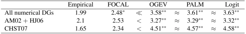
This observation is intuitively linked to both, limited attention and focal choice. Lim-ited attention presumes that only a subset of options is considered, and focal choice pre-sumes that a (limited) number of options have elevated focality. To evaluate whether this stylized fact is explained by the models, I use the estimates obtained above and compute the predicted entropy in the various treatments. The significance of differences between predicted and observed entropies is evaluated in Wilcoxon matched pairs tests. The re-sults are reported in Table 4 and confirm that both limited attention (PALM) and Ordered GEV slightly improve on logit in capturing the observed choice patterns, but are far from being compatible with the extent of the round-number effects. In turn, FOCAL is compat-ible with it in the sense that the predicted entropy, while being slightly too large,13 is not significantly different from the observed entropy.

Result 2(Entropy). FOCAL consistently captures entropy in numerical choice.

12_{Detailed overviews of these statistics are provided in the supplementary material. To compute these}

numbers for FKM07 (where budget sets are random between subjects), choicesxiare transformed to shares

transfered, i.e.xi/maxx, for each decision and rounded to multiples of 0.01.

13_{Intuitively, this relates to the noise in the data, which is unpredictable ex-ante but manifests as specific}

(20)

[image:20.595.90.505.137.195.2]

Table 4: Is entropy reliably captured?

Empirical FOCAL OGEV PALM Logit

All numerical DGs 1.99 2.48∗ _≪ _3.58∗∗ _≈ _3.61∗∗ _≈ _3.63∗∗

AM02+HJ06 2.1 2.53 < 3.27∗∗ _≈ _3.29∗∗ _≈ _3.32∗∗

CHST07 1.65 2.34 < 4.51∗∗ _≈ _4.57∗∗ _≈ _4.58∗∗

Content: This table relates the empirical entropy (estimated entropy averaged across all treatments in the respective experiments) to the respective predictions of the four choice models. The results are either pooled across all numerical DG experiments or reported for the large/small DG experiments (AM02+HJ06 or CHST07, resp.). Differences are evaluated by Wilcoxon tests, the notation of relation signs is as in Table 3. The “stars” indicate that the model’s prediction differ significantly from the empirical estimate; significance at 0.005 is indicated by∗∗_{and significance at 0.05 is indicated by}∗_.

5 Reliability and consistency

The basic hypothesis formulated above was that if the choice model does not capture the presentation effects, preference estimates are biased and inconsistent across studies. For, presentation affects focality, which in turn affects choice propensities—and if focality is not controlled for, its effect on choice propensities will bias utility estimates. The predicted bias can be econometrically tested, as it diminishes the reliability of predictions and the consistency of estimates across experiments, which is the scope of the present section.

The evaluation of predictive adequacy is the arguably most widely accepted approach to model validation, being an integral part of the scientific method, and has a tradition also in behavioral economics. Most notably, risk preferences tend to be evaluated by predictive adequacy, e.g. Harless and Camerer (1994), Wilcox (2008), Dave et al. (2010), and Hey et al. (2010), but similarly so models of learning (Camerer and Ho, 1999), time preferences (Keller and Strazzera, 2002), and strategic reasoning (Camerer et al., 2004). In the context of social preferences, however, the only study attempting an assessment of predictive ad-equacy appears to be Breitmoser (2013). This is somewhat surprising, as the instability of estimates of social preferences is notorious, but predicting say dictator behavior requires prediction of numerical choice. Thus, any result on differences across experiments would have to be ascribed to say round-number effects if those are not adequately captured, ren-dering analyses of predictive adequacy in dictator games uninformative. This implies, however, that we cannot assess the reliability of preference measurement so far.14

To give an idea of reliability, Table 5 provides the estimated mean degrees of altruism and efficiency concerns.15 The mean degree of efficiency concerns is similar across mod-els and data sets, being close to zero (i.e. Cobb-Douglas). The mean degree of altruism varies substantially across data sets. The estimates of logit, PALM and OGEV range from roughly−0.1 to 0.5, which is volatile given the general bounds of −0.5 and 0.5. The

ex-14_{In addition, behavior is qualitatively robust across dictator game experiments (Camerer, 2003), fueling}

the prior that preferences are constant across experiments and reducing the need for statistical analysis of their actual stability. Such analyses are required to assess the instability of preferences across games, though.

(21)

[image:21.595.101.497.137.226.2]

Table 5: Mean degrees of altruismαand efficiency concernsβ

FOCAL OGEV PALM Logit

α β α β α β α β

AM02 0.08 0.17 -0.13 -0.16 -0.27 0.25 -0.07 -1.69 HJ06 0.23 -0.67 0.13 -0.6 0.17 -0.65 0.17 -0.65 FKM07 0.02 0.26 0.15 -0.17 0.01 0.24 0.01 0.24 CHST07 0.16 -0.14 0.5 -0.62 0.5 -0.62 0.5 -0.62

Content: This table reports the estimated means of the degree of altruism (α) and the degree of equity concerns (β). The estimates are given for each choice model (Logit, OGEV, PALM, FOCAL) and each data set. The estimated standard errors are mostly rather close to zero and skipped for readability of this table. The are reported in the tables toward the end of the supplementary material.

treme estimates result in the experiments with the most pronounced round-number effects (i.e. with the lowest entropy),−0.1 in AM02 and 0.5 in CHST07. In contrast, FOCAL’s estimates are fairly robust, ranging from 0.02 to 0.23.16 The main question is now: Do these estimates differ across data sets? Standard errors are skipped in Table 5 and rele-gated to the supplement, as they are not informative to answer the question. An answer requires the joint evaluation of four preference parameters and it requires us to control for both precisionλand choice biasκ. These concerns are addressed in likelihood ratio tests, and as before, I use the robust test of Schennach and Wilhelm (2014).

5.1 Counterfactual reliability of estimates

Assume we have a data set examining behavior in one set of conditions and wish to predict behavior in related conditions. The reliability of such counterfactual predictions is critical for policy recommendations about say tax rates and choice interfaces (nudging). In appli-cations we might have more or less information about the target environment, i.e about precisionλand biasκof DMs in the counterfactual scenario. To reflect this possibility, and to check robustness in this respect, I distinguish counterfactual reliability to three degrees. The first degree is the reliability of the preferences estimates as such (distributions of α

andβ), while precision and choice bias (distributions ofλandκ) are assumed to be known for the target environment. This yields an understanding of the reliability of preference estimates in isolation. The second degree requires that precision is to be predicted as well, and only choice bias is assumed to be known, and the third degree requires out-of-sample prediction also of the choice bias (i.e. of all parameters). For clarity, let me formalize this.

Definition 6(Counterfactual reliability). Given data setsDinandDout, let(αin,βin,λin,κin)

and(αout,βout,λout,κout)denote the respective ML estimates (e.g.αinis the duple of mean

and variance ofα in-sample). Given a parameter vector, let BIC(α,β,λ,κ|D)denote its

16_{Note that this is the case for the assumption that utility is based on the tokens earned in the experiment,}

(22)

[image:22.595.63.534.152.334.2]

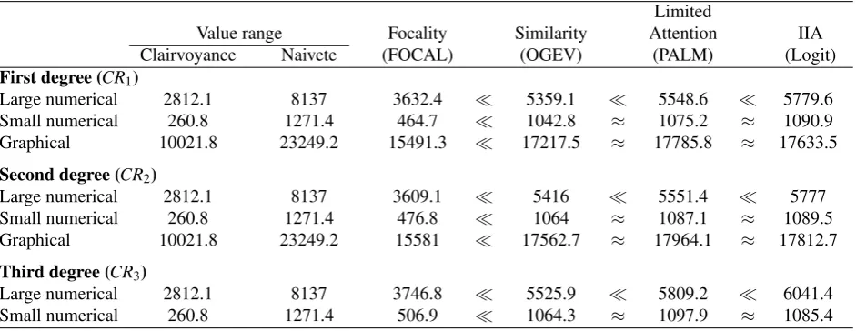
Table 6: Counterfactual reliability of estimates: How reliable are predictions of behavior in numerical and graphical experiments, based on estimates from the other experiments?

Limited

First degree (CR₁)

Large numerical 2812.1 8137 3632.4 ≪ 5359.1 ≪ 5548.6 ≪ 5779.6 Small numerical 260.8 1271.4 464.7 ≪ 1042.8 ≈ 1075.2 ≈ 1090.9 Graphical 10021.8 23249.2 15491.3 ≪ 17217.5 ≈ 17785.8 ≈ 17633.5

Second degree (CR2)

Large numerical 2812.1 8137 3609.1 ≪ 5416 ≪ 5551.4 ≪ 5777 Small numerical 260.8 1271.4 476.8 ≪ 1064 ≈ 1087.1 ≈ 1089.5 Graphical 10021.8 23249.2 15581 ≪ 17562.7 ≈ 17964.1 ≈ 17812.7

Third degree (CR3)

Large numerical 2812.1 8137 3746.8 ≪ 5525.9 ≪ 5809.2 ≪ 6041.4 Small numerical 260.8 1271.4 506.9 ≪ 1064.3 ≈ 1097.9 ≈ 1085.4

Content: This table evaluates the accuracy of predicting behavior in either “large numerical” experiments (Dout=AM02, HJ06), “small numerical” experiment (Dout=CHST07) or “graphical” experiment (Dout=

FKM07), using estimates from the respective other studies. As before,≈indicates p-values above 0.05, >, <indicatep-values between 0.005 and 0.05, and≫,≪indicatep-values below 0.005.

Bayes Information Criterion evaluated on data setD, using the correct number of

parame-ters fitted to data setD. Then, the three degrees of counterfactual reliability are

1. Preferences: CR1(Din,Dout) =BIC αin,βin,λout,κout|Dout

(17) 2. Pref & Prec: CR2(Din,Dout) =BIC αin,βin,λin,κout|Dout

(18) 3. All parameters: CR3(Din,Dout) =BIC αin,βin,λin,κin|Dout

(19)

To determine counterfactual reliability to the first and second degree, I analyze pre-dictions across numerical and graphical experiments. Counterfactual reliability to the third degree entails prediction of choice biasκ, i.e. predicting the extent of round-number ef-fects. It cannot be evaluated between numerical and graphical experiments, as the latter had been explicitly designed to neutralize the choice bias. Hence, I focus on the numer-ical experiments in the evaluation of counterfactual reliability to the third degree. For convenience, the results are aggregated to present the average accuracy of predicting a given experiment using estimates from the other experiments. Formally, given degreek, the reliability in predictingDoutisCRk(Dout) =∑Din=6 DoutCRk(Din,Dout)/3. The classes of

experiments are labeled large numerical, small numerical, and graphical, as above.

(23)

nu-merical choice, and mostly between 0.4 and 0.5 for the other models in case of nunu-merical choice. In addition to the high statistical significance, two observations specifically sug-gest that FOCAL captures choice and thus measures preferences reliably. On the one hand, the models are differently adequate in predicting graphical choice. Predicting graphical choice represents the arguably cleanest test of counterfactual reliability: graphical choice does not exhibit round-number effects, all models are equally adequate in-sample, and thus all differences in reliability stem from inaccurate measurement of preferences in the other data sets. The higher adequacy of FOCAL in predicting graphical choice thus shows that its preference estimates are more reliable.

On the other hand, the reliability of counterfactual predictions depends only marginally on our knowledge of the target environment. In particular, the precision of subjects is pre-dicted reliably, i.e. it represents a robust facet of behavior, and accuracy drops only slightly (between two and four percentage points in the pseudo-R2) if we have to predict even the

extent of the choice bias. In applications, neither precision nor choice bias therefore need to be known for the target environment. This is largely trivial for all models but FOCAL, as those do not capture the choice bias. As for FOCAL, however, this shows that its de-composition of behavior into utility and focality provides a measurement of choice factors that is both accurate and robust across choice environments.

Result 3. Counterfactual predictions are most reliable for FOCAL, for all user interfaces and regardless of how much we know about the target environment.

5.2 External consistency of estimates

Now assume we have two data sets and wish to examine if preferences in one data set differ from those in the other data set. I refer to this as test of the consistency of preferences. Consistency of estimates across experiments on a given game is a necessary condition for reliably understanding differences between games. If estimates are inconsistent, e.g. if preferences are found to significantly depend on presentation, results on differences of estimates between classes of games would not be informative—they could either reflect actual changes in utility or pure presentation biases.

To evaluate estimate consistency, the relevant likelihood ratio is the difference of log-likelihoods in-sample and out-of-sample. That is, we take estimates from a data set

Din, predictDout, and compare the respective likelihood (or, BIC) to the one achieved

in-sample inDout. As above, I distinguish consistency to the three degrees: consistency of

preference estimates in isolation, consistency of preference and precision estimates jointly, and consistency of all estimates jointly.

Definition 7(Estimate consistency). Given data setsDinandDout, let(αin,βin,λin,κin)and

(αout,βout,λout,κout)denote the respective ML estimates (e.g.αin is the duple of mean and

(24)

[image:24.595.61.536.137.319.2]

Table 7: Estimate consistency: How different are estimates between experiments?

Limited

First degree (EC1)

Large numerical 0 22737.7 531.4 ≪ 1601.6∗ _< _2188.6∗∗ _> ₁₆₅₅∗

Small numerical 0 12910.4 1377.9∗ _≪ ₇₁₁₁∗∗ _≪ _8738.5∗∗ _≈ _8890.6∗∗

Graphical 0 5606 137.4 ≪ 859.6∗∗ _> _733.7∗∗ _≈ _730.4∗∗

Second degree (EC2)

Large numerical 0 22737.7 854.9 ≪ 1825.5∗∗ _< _2327.2∗∗ _> _1755.7∗∗

Small numerical 0 12910.4 1275.7∗ _≪ _8108.3∗∗ _≪ _9252.4∗∗ _≈ _9359.2∗∗

Graphical 0 5606 151.4 ≪ 908.3∗∗ _≫ _660.4∗∗ _≈ _686.7∗∗

Third degree (EC3)

Large numerical 0 6447 235.5∗ _≪ _806.3∗∗ _≈ ₇₄₆∗∗ _≈ _703.3∗∗

Small numerical 0 4765.1 667∗∗ _≪ _1692.2∗∗ _≪ ₂₂₆₂∗∗ _≈ _2307.5∗∗

Content: This table evaluates consistency of estimates from either “large numerical” experiments (Din=

AM02, HJ06), “small numerical” experiment (Din=CHST07) or “graphical” experiment (Din=FKM07),

in relation to estimates from the respective other studies. As before,≈indicatesp-values above 0.05,>, < indicatep-values between 0.005 and 0.05, and≫,≪indicatep-values below 0.005. Further, “stars”

indi-cate the significance of inconsistency; significance at 0.005 is indiindi-cated by∗∗_{and significance at 0.05 by}∗_. Note:The third degree does not involve predictions of the graphical experiment (FKM07). Thus, the

num-bers are not directly comparable to the other degrees.

fitted to data setD. Then, the three degrees of estimate consistency are

EC1(Din,Dout) =BIC αin,βin,λout,κout|Dout

−BIC αout,βout,λout,κout|Dout

(20)

EC2(Din,Dout) =BIC αin,βin,λin,κout|Dout

−BIC αout,βout,λout,κout|Dout

(21)

EC3(Din,Dout) =BIC αin,βin,λin,κin|Dout−BIC αout,βout,λout,κout|Dout (22)

The results are presented in Table 7, aggregated again based on user interface. Now, given degreek, we evaluate the consistency of the estimates fromDin, which is defined as

ECk(Din) =∑Dout6=DinECk(Din,Dout). That is, for a given vector of estimates, we analyze

how it explains behavior in other experiments. This is complementary to the analysis of counterfactual reliability, which is the reliability of predicting a given data set using estimates from other data sets. The inversion feels natural in evaluating consistency and provides a complementary perspective on the results, facilitating their interpretation.