Mine the Easy, Classify the Hard:
A Semi-Supervised Approach to Automatic Sentiment Classification
Sajib Dasgupta and Vincent Ng
Human Language Technology Research Institute University of Texas at Dallas
Richardson, TX 75083-0688
{sajib,vince}@hlt.utdallas.edu
Abstract
Supervised polarity classification systems are typically domain-specific. Building these systems involves the expensive pro-cess of annotating a large amount of data for each domain. A potential solution to this corpus annotation bottleneck is to build unsupervised polarity classification systems. However, unsupervised learning of polarity is difficult, owing in part to the prevalence of sentimentally ambiguous re-views, where reviewers discuss both the positive and negative aspects of a prod-uct. To address this problem, we pro-pose a semi-supervised approach to senti-ment classification where we first mine the unambiguous reviews using spectral tech-niques and then exploit them to classify the ambiguous reviews via a novel com-bination of active learning, transductive learning, and ensemble learning.
1 Introduction
Sentiment analysis has recently received a lot of attention in the Natural Language Processing (NLP) community. Polarity classification, whose goal is to determine whether the sentiment ex-pressed in a document is “thumbs up” or “thumbs down”, is arguably one of the most popular tasks in document-level sentiment analysis. Unlike topic-based text classification, where a high accu-racy can be achieved even for datasets with a large number of classes (e.g., 20 Newsgroups), polarity classification appears to be a more difficult task. One reason topic-based text classification is easier than polarity classification is that topic clusters are typically well-separated from each other, result-ing from the fact that word usage differs consid-erably between two topically-different documents. On the other hand, many reviews are sentimentally
ambiguous for a variety of reasons. For instance,
an author of a movie review may have negative opinions of the actors but at the same time talk enthusiastically about how much she enjoyed the plot. Here, the review is ambiguous because she discussed both the positive and negative aspects of the movie, which is not uncommon in reviews. As another example, a large portion of a movie re-view may be devoted exclusively to the plot, with the author only briefly expressing her sentiment at the end of the review. In this case, the review is ambiguous because the objective material in the review, which bears no sentiment orientation, sig-nificantly outnumbers its subjective counterpart.
Realizing the challenges posed by ambiguous reviews, researchers have explored a number of techniques to improve supervised polarity classi-fiers. For instance, Pang and Lee (2004) train an independent subjectivity classifier to identify and remove objective sentences from a review prior to polarity classification. Koppel and Schler (2006) use neutral reviews to help improve the classi-fication of positive and negative reviews. More recently, McDonald et al. (2007) have investi-gated a model for jointly performing sentence- and document-level sentiment analysis, allowing the relationship between the two tasks to be captured and exploited. However, the increased sophistica-tion of supervised polarity classifiers has also re-sulted in their increased dependence on annotated data. For instance, Koppel and Schler needed to manually identify neutral reviews to train their po-larity classifier, and McDonald et al.’s joint model requires that each sentence in a review be labeled with polarity information.
Given the difficulties of supervised polarity classification, it is conceivable that unsupervised polarity classification is a very challenging task. Nevertheless, a solution to unsupervised polarity classification is of practical significance. One rea-son is that the vast majority of supervised polarity
classification systems are domain-specific. Hence, when given a new domain, a large amount of an-notated data from the domain typically needs to be collected in order to train a high-performance po-larity classification system. As Blitzer et al. (2007) point out, this data collection process can be “pro-hibitively expensive, especially since product fea-tures can change over time”. Unfortunately, to our knowledge, unsupervised polarity classifica-tion is largely an under-investigated task in NLP. Turney’s (2002) work is perhaps one of the most notable examples of unsupervised polarity clas-sification. However, while his system learns the semantic orientation of phrases in a review in an unsupervised manner, such information is used to heuristically predict the polarity of a review.
At first glance, it may seem plausible to apply an unsupervised clustering algorithm such as k -means to cluster the reviews according to their po-larity. However, there is reason to believe that such a clustering approach is doomed to fail: in the ab-sence of annotated data, an unsupervised learner is unable to identify which features are relevant for polarity classification. The situation is further complicated by the prevalence of ambiguous re-views, which may contain a large amount of irrel-evant and/or contradictory information.
In light of the difficulties posed by ambiguous reviews, we differentiate between ambiguous and unambiguous reviews in our classification process by addressing the task of semi-supervised polar-ity classification via a “mine the easy, classify the hard” approach. Specifically, we propose a novel system architecture where we first automatically identify and label the unambiguous (i.e., “easy”) reviews, then handle the ambiguous (i.e., “hard”) reviews using a discriminative learner to bootstrap from the automatically labeled unambiguous views and a small number of manually labeled re-views that are identified by an active learner.
It is worth noting that our system differs from existing work on unsupervised/active learning in two aspects. First, while existing unsupervised approaches typically rely on clustering or learn-ing via a generative model, our approach distin-guishes between easy and hard instances and ex-ploits the strengths of discriminative models to classify the hard instances. Second, while exist-ing active learners typically start with manually la-beled seeds, our active learner relies only on seeds that are automatically extracted from the data.
Ex-perimental results on five sentiment classification datasets demonstrate that our system can gener-ate high-quality labeled data from unambiguous reviews, which, together with a small number of manually labeled reviews selected by the active learner, can be used to effectively classify ambigu-ous reviews in a discriminative fashion.
The rest of the paper is organized as follows. Section 2 gives an overview of spectral cluster-ing, which will facilitate the presentation of our approach to unsupervised sentiment classification in Section 3. We evaluate our approach in Section 4 and present our conclusions in Section 5.
2 Spectral Clustering
In this section, we give an overview of spectral clustering, which is at the core of our algorithm for identifying ambiguous reviews.
2.1 Motivation
When given a clustering task, an important ques-tion to ask is: which clustering algorithm should be used? A popular choice isk-means. Neverthe-less, it is well-known thatk-means has the major drawback of not being able to separate data points that are not linearly separable in the given feature space (e.g, see Dhillon et al. (2004)). Spectral clustering algorithms were developed in response to this problem withk-means clustering. The cen-tral idea behind speccen-tral clustering is to (1) con-struct a low-dimensional space from the original (typically high-dimensional) space while retaining as much information about the original space as possible, and (2) cluster the data points in this low-dimensional space.
2.2 Algorithm
Although there are several well-known spectral clustering algorithms in the literature (e.g., Weiss (1999), Meil˘a and Shi (2001), Kannan et al. (2004)), we adopt the one proposed by Ng et al. (2002), as it is arguably the most widely used. The algorithm takes as input a similarity matrixS cre-ated by applying a user-defined similarity function to each pair of data points. Below are the main steps of the algorithm:
1. Create the diagonal matrix G whose (i,i )-th entry is )-the sum of )-the i-th row of S, and then construct the Laplacian matrixL =
G−1/2SG−1/2
.
3. Create a new matrix from themeigenvectors that correspond to themlargest eigenvalues.1
4. Each data point is now rank-reduced to a point in them-dimensional space. Normal-ize each point to unit length (while retaining the sign of each value).
5. Cluster the resulting data points using k -means.
In essence, each dimension in the reduced space is defined by exactly one eigenvector. The rea-son why eigenvectors with large eigenvalues are retained is that they capture the largest variance in the data. Therefore, each of them can be thought of as revealing an important dimension of the data.
3 Our Approach
While spectral clustering addresses a major draw-back of k-means clustering, it still cannot be ex-pected to accurately partition the reviews due to the presence of ambiguous reviews. Motivated by this observation, rather than attempting to cluster
all the reviews at the same time, we handle them in
different stages. As mentioned in the introduction, we employ a “mine the easy, classify the hard” approach to polarity classification, where we (1) identify and classify the “easy” (i.e., unambigu-ous) reviews with the help of a spectral cluster-ing algorithm; (2) manually label a small number of “hard” (i.e., ambiguous) reviews selected by an active learner; and (3) using the reviews labeled thus far, apply a transductive learner to label the remaining (ambiguous) reviews. In this section, we discuss each of these steps in detail.
3.1 Identifying Unambiguous Reviews
We begin by preprocessing the reviews to be clas-sified. Specifically, we tokenize and downcase each review and represent it as a vector of uni-grams, using frequency as presence. In addition, we remove from the vector punctuation, numbers, words of length one, and words that occur in a single review only. Finally, following the com-mon practice in the information retrieval commu-nity, we remove words with high document fre-quency, many of which are stopwords or domain-specific general-purpose words (e.g., “movies” in the movie domain). A preliminary examination of our evaluation datasets reveals that these words
1For brevity, we will refer to the eigenvector with the
n-th
largest eigenvalue simply as then-th eigenvector.
typically comprise 1–2% of a vocabulary. The de-cision of exactly how many terms to remove from each dataset is subjective: a large corpus typically requires more removals than a small corpus. To be consistent, we simply sort the vocabulary by doc-ument frequency and remove the top 1.5%.
Recall that in this step we use spectral clustering to identify unambiguous reviews. To make use of spectral clustering, we first create a similarity ma-trix, defining the similarity between two reviews as the dot product of their feature vectors, but fol-lowing Ng et al. (2002), we set its diagonal entries to 0. We then perform an eigen-decomposition of this matrix, as described in Section 2.2. Finally, using the resulting eigenvectors, we partition the length-normalized reviews into two sets.
As Ng et al. point out, “different authors still disagree on which eigenvectors to use, and how to derive clusters from them”. To create two clusters, the most common way is to use only the second eigenvector, as Shi and Malik (2000) proved that this eigenvector induces an intuitively ideal par-tition of the data — the parpar-tition induced by the minimum normalized cut of the similarity graph2, where the nodes are the data points and the edge weights are the pairwise similarity values of the points. Clustering in a one-dimensional space is trivial: since we have a linearization of the points, all we need to do is to determine a threshold for partitioning the points. A common approach is to set the threshold to zero. In other words, all points whose value in the second eigenvector is positive are classified as positive, and the remaining points are classified as negative. However, we found that the second eigenvector does not always induce a partition of the nodes that corresponds to the min-imum normalized cut. One possible reason is that Shi and Malik’s proof assumes the use of a Lapla-cian matrix that is different from the one used by Ng et al. To address this problem, we use the first five eigenvectors: for each eigenvector, we (1) use each of itsn elements as a threshold to indepen-dently generate npartitions, (2) compute the nor-malized cut value for each partition, and (3) find the minimum of the ncut values. We then select the eigenvector that corresponds to the smallest of the five minimum cut values.
Next, we identify the ambiguous reviews from
2Using the normalized cut (as opposed to the usual cut)
the resulting partition. To see how this is done, consider the example in Figure 1, where the goal is to produce two clusters from five data points.
1 1 1 0 0 1 1 1 0 0 0 0 1 1 0 0 0 0 1 1 0 0 0 1 1
! −0.6983 0.7158
−0.6983 0.7158
−0.9869−0.1616
−0.6224−0.7827
−0.6224−0.7827
!
Figure 1: Sample data and the top two eigenvec-tors of its Laplacian
In the matrix on the left, each row is the feature vector generated forDi, thei-th data point. By
in-spection, one can identify two clusters, {D1, D2}
and {D4, D5}. D3 is ambiguous, as it bears
re-semblance to the points in both clusters and there-fore can be assigned to any of them. In the ma-trix on the right, the two columns correspond to the top two eigenvectors obtained via an eigen-decomposition of the Laplacian matrix formed from the five data points. As we can see, the sec-ond eigenvector gives us a natural cluster assign-ment: all the points whose corresponding values in the second eigenvector are strongly positive will be in one cluster, and the strongly negative points will be in another cluster. Being ambiguous,D3is
weakly negative and will be assigned to the
“neg-ative” cluster. Before describing our algorithm for identifying ambiguous data points, we make two additional observations regarding D3.
First, if we removedD3, we could easily
clus-ter the remaining (unambiguous) points, since the similarity graph becomes more disconnected as we remove more ambiguous data points. The question then is: why is it important to produce a good clustering of the unambiguous points? Re-call that the goal of this step is not only to
iden-tify the unambiguous reviews, but also to annotate
them asPOSITIVE orNEGATIVE, so that they can serve as seeds for semi-supervised learning in a later step. If we have a good 2-way clustering of the seeds, we can simply annotate each cluster (by sampling a handful of its reviews) rather than each seed. To reiterate, removing the ambiguous data points can help produce a good clustering of their unambiguous counterparts.
Second, as an ambiguous data point,D3 can in
principle be assigned to any of the two clusters. According to the second eigenvector, it should be assigned to the “negative” cluster; but if feature #4 were irrelevant, it should be assigned to the “positive” cluster. In other words, the ability to determine the relevance of each feature is crucial
to the accurate clustering of the ambiguous data points. However, in the absence of labeled data, it is not easy to assess feature relevance. Even if labeled data were present, the ambiguous points might be better handled by a discriminative learn-ing system than a clusterlearn-ing algorithm, as discrim-inative learners are more sophisticated, and can handle ambiguous feature space more effectively.
Taking into account these two observations, we aim to (1) remove the ambiguous data points while clustering their unambiguous counterparts, and then (2) employ a discriminative learner to label the ambiguous points in a later step.
The question is: how can we identify the ambiguous data points? To do this, we ex-ploit an important observation regarding eigen-decomposition. In the computation of eigenvalues, each data point factors out the orthogonal projec-tions of each of the other data points with which they have an affinity. Ambiguous data points re-ceive the orthogonal projections from both the positive and negative data points, and hence they have near-zero values in the pivot eigenvectors. Given this observation, our algorithm uses the eight steps below to remove the ambiguous points in an iterative fashion and produce a clustering of the unambiguous points.
1. Create a similarity matrix S from the data pointsD.
2. Form the Laplacian matrixLfromS. 3. Find the top five eigenvectors ofL. 4. Row-normalize the five eigenvectors.
5. Pick the eigenvector efor which we get the minimum normalized cut.
6. SortDaccording toeand removeαpoints in the middle ofD(i.e., the points indexed from
|D|
2 −
α 2 + 1to
|D|
2 +
α 2).
7. If|D|=β, goto Step 8; else goto Step 1. 8. Run 2-means oneto cluster the points inD.
single iteration): the clusters produced in a given iteration are supposed to be better than those in the previous iterations, as subsequent clusterings are generated from less ambiguous points. In our experiments, we setαto 50 andβto 500.3
Finally, we label the two clusters. To do this, we first randomly sample 10 reviews from each cluster and manually label each of them as POS
-ITIVE orNEGATIVE. Then, we label a cluster as
POSITIVEif more than half of the 10 reviews from
the cluster are POSITIVE; otherwise, it is labeled
asNEGATIVE. For each of our evaluation datasets,
this labeling scheme always produces one POSI
-TIVEcluster and oneNEGATIVEcluster. In the rest of the paper, we will refer to these 500 automati-cally labeled reviews as seeds.
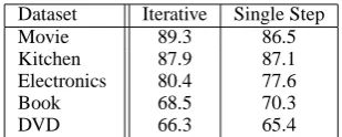
A natural question is: can this algorithm pro-duce high-quality seeds? To answer this question, we show in the middle column of Table 1 the label-ing accuracy of the 500 reviews produced by our iterative algorithm for our five evaluation datasets (see Section 4.1 for details on these datasets). To better understand whether it is indeed beneficial to remove the ambiguous points in an iterative fashion, we also show the results of a version of this algorithm in which we remove all but the 500 least ambiguous points in just one iteration (see the rightmost column). As we can see, for three datasets (Movie, Kitchen, and Electronics), the accuracy is above 80%. For the remaining two (Book and DVD), the accuracy is not particularly good. One plausible reason is that the ambiguous reviews in Book and DVD are relatively tougher to identify. Another reason can be attributed to the failure of the chosen eigenvector to capture the sentiment dimension. Recall that each eigenvector captures an important dimension of the data, and if the eigenvector that corresponds to the minimum normalized cut (i.e., the eigenvector that we chose) does not reveal the sentiment dimension, the re-sulting clustering (and hence the seed accuracy) will be poor. However, even with imperfectly la-beled seeds, we will show in the next section how we exploit these seeds to learn a better classifier.
3.2 Incorporating Active Learning
Spectral clustering allows us to focus on a small number of dimensions that are relevant as far as creating well-separated clusters is concerned, but
3Additional experiments indicate that the accuracy of our
approach is not sensitive to small changes to these values.
Dataset Iterative Single Step
Movie 89.3 86.5
Kitchen 87.9 87.1
Electronics 80.4 77.6
Book 68.5 70.3
[image:5.595.339.494.61.123.2]DVD 66.3 65.4
Table 1: Seed accuracies on five datasets.
they are not necessarily relevant for creating po-larity clusters. In fact, owing to the absence of la-beled data, unsupervised clustering algorithms are unable to distinguish between useful and irrelevant features for polarity classification. Nevertheless, being able to distinguish between relevant and ir-relevant information is important for polarity clas-sification, as discussed before. Now that we have a small, high-quality seed set, we can potentially make better use of the available features by train-ing a discriminative classifier on the seed set and having it identify the relevant and irrelevant fea-tures for polarity classification.
Despite the high quality of the seed set, the re-sulting classifier may not perform well when ap-plied to the remaining (unlabeled) points, as there is no reason to believe that a classifier trained solely on unambiguous reviews can achieve a high accuracy when classifying ambiguous re-views. We hypothesize that a high accuracy can be achieved only if the classifier is trained on both ambiguous and unambiguous reviews.
As a result, we apply active learning (Cohn et al., 1994) to identify the ambiguous reviews. Specifically, we train a discriminative classifier us-ing the support vector machine (SVM) learnus-ing al-gorithm (Joachims, 1999) on the set of unambigu-ous reviews, and then apply the resulting classifier to all the reviews in the training folds4that are not seeds. Since this classifier is trained solely on the unambiguous reviews, it is reasonable to assume that the reviews whose labels the classifier is most uncertain about (and therefore are most informa-tive to the classifier) are those that are ambigu-ous. Following previous work on active learning for SVMs (e.g., Campbell et al. (2000), Schohn and Cohn (2000), Tong and Koller (2002)), we de-fine the uncertainty of a data point as its distance from the separating hyperplane. In other words,
4Following Dredze and Crammer (2008), we perform
points that are closer to the hyperplane are more uncertain than those that are farther away.
We perform active learning for five iterations. In each iteration, we select the 10 most uncertain points from each side of the hyperplane for human annotation, and then re-train a classifier on all of the points annotated so far. This yields a total of 100 manually labeled reviews.
3.3 Applying Transductive Learning
Given that we now have a labeled set (composed of 100 manually labeled points selected by active learning and 500 unambiguous points) as well as a larger set of points that are yet to be labeled (i.e., the remaining unlabeled points in the train-ing folds and those in the test fold), we aim to train a better classifier by using a weakly super-vised learner to learn from both the labeled and unlabeled data. As our weakly supervised learner, we employ a transductive SVM.
To begin with, note that the automatically ac-quired 500 unambiguous data points are not per-fectly labeled (see Section 3.1). Since these unam-biguous points significantly outnumber the manu-ally labeled points, they could undesirably domi-nate the acquisition of the hyperplane and dimin-ish the benefits that we could have obtained from the more informative and perfectly labeled active learning points otherwise. We desire a system that can use the active learning points effectively and at the same time is noise-tolerant to the imperfectly labeled unambiguous data points. Hence, instead of training just one SVM classifier, we aim to re-duce classification errors by training an ensemble of five classifiers, each of which uses all 100 man-ually labeled reviews and a different subset of the 500 automatically labeled reviews.
Specifically, we partition the 500 automatically labeled reviews into five equal-sized sets as fol-lows. First, we sort the 500 reviews in ascending order of their corresponding values in the eigen-vector selected in the last iteration of our algorithm for removing ambiguous points (see Section 3.1). We then put pointiinto setLimod 5. This ensures
that each set consists of not only an equal number of positive and negative points, but also a mix of very confidently labeled points and comparatively less confidently labeled points. Each classifierCi
will then be trained transductively, using the 100 manually labeled points and the points inLias la-beled data, and the remaining points (including all
points inLj, wherei6=j) as unlabeled data.
After training the ensemble, we classify each unlabeled point as follows: we sum the (signed) confidence values assigned to it by the five ensem-ble classifiers, labeling it as POSITIVE if the sum is greater than zero (and NEGATIVE otherwise).
Since the points in the test fold are included in the unlabeled data, they are all classified in this step.
4 Evaluation
4.1 Experimental Setup
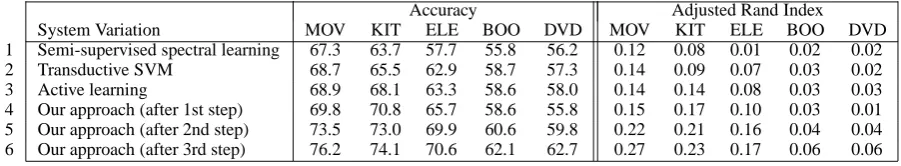
For evaluation, we use five sentiment classifica-tion datasets, including the widely-used movie re-view dataset [MOV] (Pang et al., 2002) as well as four datasets that contain reviews of four differ-ent types of product from Amazon [books (BOO), DVDs (DVD), electronics (ELE), and kitchen ap-pliances (KIT)] (Blitzer et al., 2007). Each dataset has 2000 labeled reviews (1000 positives and 1000 negatives). We divide the 2000 reviews into 10 equal-sized folds for cross-validation purposes, maintaining balanced class distributions in each fold. It is important to note that while the test fold is accessible to the transductive learner (Step 3), only the reviews in training folds (but not their la-bels) are used for the acquisition of seeds (Step 1) and the selection of active learning points (Step 2). We report averaged 10-fold cross-validation re-sults in terms of accuracy. Following Kamvar et al. (2003), we also evaluate the clusters produced by our approach against the gold-standard clusters us-ing Adjusted Rand Index (ARI). ARI ranges from −1 to 1; better clusterings have higher ARI values.
4.2 Baseline Systems
Accuracy Adjusted Rand Index
System Variation MOV KIT ELE BOO DVD MOV KIT ELE BOO DVD
1 Semi-supervised spectral learning 67.3 63.7 57.7 55.8 56.2 0.12 0.08 0.01 0.02 0.02
2 Transductive SVM 68.7 65.5 62.9 58.7 57.3 0.14 0.09 0.07 0.03 0.02
3 Active learning 68.9 68.1 63.3 58.6 58.0 0.14 0.14 0.08 0.03 0.03
4 Our approach (after 1st step) 69.8 70.8 65.7 58.6 55.8 0.15 0.17 0.10 0.03 0.01
5 Our approach (after 2nd step) 73.5 73.0 69.9 60.6 59.8 0.22 0.21 0.16 0.04 0.04
[image:7.595.76.527.62.145.2]6 Our approach (after 3rd step) 76.2 74.1 70.6 62.1 62.7 0.27 0.23 0.17 0.06 0.06
Table 2: Results in terms of accuracy and Adjusted Rand Index for the five datasets.
k, we tested values of 10, 15,. . ., 50 forkand re-ported in row 1 of Table 2 the best results. As we can see, accuracy ranges from 56.2% to 67.3%, whereas ARI ranges from 0.02 to 0.12.
Transductive SVM. We employ as our second baseline a transductive SVM5 trained using 100 points randomly sampled from the training folds as labeled data and the remaining 1900 points as unlabeled data. Results of this baseline are shown in row 2 of Table 3. As we can see, accuracy ranges from 57.3% to 68.7% and ARI ranges from 0.02 to 0.14, which are significantly better than those of semi-supervised spectral learning.
Active learning. Our last baseline implements the active learning procedure as described in Tong and Koller (2002). Specifically, we begin by train-ing an inductive SVM on one labeled example from each class, iteratively labeling the most un-certain unlabeled point on each side of the hyper-plane and re-training the SVM until 100 points are labeled. Finally, we train a transductive SVM on the 100 labeled points and the remaining 1900 un-labeled points, obtaining the results in row 3 of Ta-ble 1. As we can see, accuracy ranges from 58% to 68.9%, whereas ARI ranges from 0.03 to 0.14. Active learning is the best of the three baselines, presumably because it has the ability to choose the labeled data more intelligently than the other two.
4.3 Our Approach
Results of our approach are shown in rows 4–6 of Table 2. Specifically, rows 4 and 5 show the re-sults of the SVM classifier when it is trained on the labeled data obtained after the first step (unsu-pervised extraction of unambiguous reviews) and the second step (active learning), respectively. Af-ter the first step, our approach can already achieve
5All the SVM classifiers in this paper are trained using
the SVMlightpackage (Joachims, 1999). All SVM-related
learning parameters are set to their default values, except in transductive learning, where we setp(the fraction of
unla-beled examples to be classified as positive) to 0.5 so that the system does not have any bias towards any class.
comparable results to the best baseline. Per-formance increases substantially after the second step, indicating the benefits of active learning.
Row 6 shows the results of transductive learn-ing with ensemble. Comparing rows 5 and 6, we see that performance rises by 0.7%-2.9% for all five datasets after “ensembled” transduction. This could be attributed to (1) the unlabeled data, which may have provided the transductive learner with useful information that are not accessible to the other learners, and (2) the ensemble, which is more noise-tolerant to the imperfect seeds.
4.4 Additional Experiments
To gain insight into how the design decisions we made in our approach impact performance, we conducted the following additional experiments.
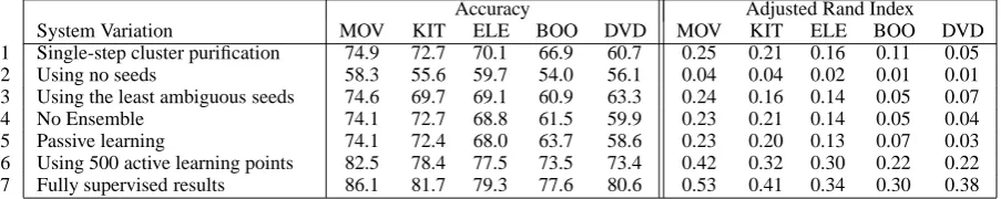
Importance of seeds. Table 1 showed that for all but one dataset, the seeds obtained through multiple iterations are more accurate than those obtained in a single iteration. To envisage the im-portance of seeds, we conducted an experiment where we repeated our approach using the seeds learned in a single iteration. Results are shown in the first row of Table 3. In comparison to row 6 of Table 2, we can see that results are indeed better when we bootstrap from higher-quality seeds.
To further understand the role of seeds, we ex-perimented with a version of our approach that bootstraps from no seeds. Specifically, we used the 500 seeds to guide the selection of active learn-ing points, but trained a transductive SVM uslearn-ing only the active learning points as labeled data (and the rest as unlabeled data). As can be seen in row 2 of Table 3, the results are poor, suggesting that our approach yields better performance than the baselines not only because of the way the active learning points were chosen, but also because of contributions from the imperfectly labeled seeds.
Accuracy Adjusted Rand Index
System Variation MOV KIT ELE BOO DVD MOV KIT ELE BOO DVD
1 Single-step cluster purification 74.9 72.7 70.1 66.9 60.7 0.25 0.21 0.16 0.11 0.05
2 Using no seeds 58.3 55.6 59.7 54.0 56.1 0.04 0.04 0.02 0.01 0.01
3 Using the least ambiguous seeds 74.6 69.7 69.1 60.9 63.3 0.24 0.16 0.14 0.05 0.07
4 No Ensemble 74.1 72.7 68.8 61.5 59.9 0.23 0.21 0.14 0.05 0.04
5 Passive learning 74.1 72.4 68.0 63.7 58.6 0.23 0.20 0.13 0.07 0.03
6 Using 500 active learning points 82.5 78.4 77.5 73.5 73.4 0.42 0.32 0.30 0.22 0.22
[image:8.595.78.530.64.154.2]7 Fully supervised results 86.1 81.7 79.3 77.6 80.6 0.53 0.41 0.34 0.30 0.38
Table 3: Additional results in terms of accuracy and Adjusted Rand Index for the five datasets.
second eigenvector values) in combination with the active learning points as labeled data (and the rest as unlabeled data). Note that the accuracy of these 100 least ambiguous seeds is 4–5% higher than that of the 500 least ambiguous seeds shown in Table 1. Results are shown in row 3 of Table 3. As we can see, using only 100 seeds turns out to be less beneficial than using all of them via an ensem-ble. One reason is that since these 100 seeds are the most unambiguous, they may also be the least informative as far as learning is concerned. Re-member that SVM uses only the support vectors to acquire the hyperplane, and since an unambiguous seed is likely to be far away from the hyperplane, it is less likely to be a support vector.
Role of ensemble learning To get a better idea of the role of the ensemble in the transductive learning step, we used all 500 seeds in combina-tion with the 100 active learning points to train a single transductive SVM. Results of this experi-ment (shown in row 4 of Table 3) are worse than those in row 6 of Table 2, meaning that the en-semble has contributed positively to performance. This should not be surprising: as noted before, since the seeds are not perfectly labeled, using all of them without an ensemble might overwhelm the more informative active learning points.
Passive learning. To better understand the role of active learning in our approach, we replaced it with passive learning, where we randomly picked 100 data points from the training folds and used them as labeled data. Results, shown in row 5 of Table 3, are averaged over ten independent runs for each fold. In comparison to row 6 of Table 2, we see that employing points chosen by an active learner yields significantly better results than em-ploying randomly chosen points, which suggests that the way the points are chosen is important.
Using more active learning points. An interest-ing question is: how much improvement can we obtain if we employ more active learning points?
In row 6 of Table 3, we show the results when the experiment in row 6 of Table 2 was repeated using 500 active learning points. Perhaps not surpris-ingly, the 400 additional labeled points yield a 4– 11% increase in accuracy. For further comparison, we trained a fully supervised SVM classifier using all of the training data. Results are shown in row 7 of Table 3. As we can see, employing only 500 active learning points enables us to almost reach fully-supervised performance for three datasets.
5 Conclusions
We have proposed a novel semi-supervised ap-proach to polarity classification. Our key idea is to distinguish between unambiguous, easy-to-mine reviews and ambiguous, hard-to-classify re-views. Specifically, given a set of reviews, we applied (1) an unsupervised algorithm to identify and classify those that are unambiguous, (2) an active learner that is trained solely on automati-cally labeled unambiguous reviews to identify a small number of prototypical ambiguous reviews for manual labeling, and (3) an ensembled trans-ductive learner to train a sophisticated classifier on the reviews labeled so far to handle the am-biguous reviews. Experimental results on five sen-timent datasets demonstrate that our “mine the easy, classify the hard” approach, which only re-quires manual labeling of a small number of am-biguous reviews, can be employed to train a high-performance polarity classification system.
Acknowledgments
We thank the three anonymous reviewers for their invaluable comments on an earlier draft of the pa-per. This work was supported in part by NSF Grant IIS-0812261.
References
John Blitzer, Mark Dredze, and Fernando Pereira. 2007. Biographies, bollywood, boom-boxes and blenders: Domain adaptation for sentiment classi-fication. In Proceedings of the ACL, pages 440–447.
Colin Campbell, Nello Cristianini, , and Alex J. Smola. 2000. Query learning with large margin classifiers. In Proceedings of ICML, pages 111–118.
David Cohn, Les Atlas, and Richard Ladner. 1994. Improving generalization with active learning.
Ma-chine Learning, 15(2):201–221.
Inderjit Dhillon, Yuqiang Guan, and Brian Kulis. 2004. Kernelk-means, spectral clustering and normalized cuts. In Proceedings of KDD, pages 551–556.
Mark Dredze and Koby Crammer. 2008. Active learn-ing with confidence. In Proceedlearn-ings of ACL-08:HLT
Short Papers (Companion Volume), pages 233–236.
Thorsten Joachims. 1999. Making large-scale SVM learning practical. In Bernhard Scholkopf and Alexander Smola, editors, Advances in Kernel
Meth-ods - Support Vector Learning, pages 44–56. MIT
Press.
Sepandar Kamvar, Dan Klein, and Chris Manning. 2003. Spectral learning. In Proceedings of IJCAI, pages 561–566.
Ravi Kannan, Santosh Vempala, and Adrian Vetta. 2004. On clusterings: Good, bad and spectral.
Jour-nal of the ACM, 51(3):497–515.
Moshe Koppel and Jonathan Schler. 2006. The im-portance of neutral examples for learning sentiment.
Computational Intelligence, 22(2):100–109.
Ryan McDonald, Kerry Hannan, Tyler Neylon, Mike Wells, and Jeff Reynar. 2007. Structured models for fine-to-coarse sentiment analysis. In Proceedings of
the ACL, pages 432–439.
Marina Meil˘a and Jianbo Shi. 2001. A random walks view of spectral segmentation. In Proceedings of
AISTATS.
Andrew Ng, Michael Jordan, and Yair Weiss. 2002. On spectral clustering: Analysis and an algorithm. In Advances in NIPS 14.
Bo Pang and Lillian Lee. 2004. A sentimental educa-tion: Sentiment analysis using subjectivity summa-rization based on minimum cuts. In Proceedings of
the ACL, pages 271–278.
Bo Pang, Lillian Lee, and Shivakumar Vaithyanathan. 2002. Thumbs up? Sentiment classification us-ing machine learnus-ing techniques. In Proceedus-ings of
EMNLP, pages 79–86.
Greg Schohn and David Cohn. 2000. Less is more: Active learning with support vector machines. In
Proceedings of ICML, pages 839–846.
Jianbo Shi and Jitendra Malik. 2000. Normalized cuts and image segmentation. IEEE Transactions on
Pat-tern Analysis and Machine Intelligence, 22(8):888–
905.
Simon Tong and Daphne Koller. 2002. Support vec-tor machine active learning with applications to text classification. Journal of Machine Learning Re-search, 2:45–66.
Peter Turney. 2002. Thumbs up or thumbs down? Se-mantic orientation applied to unsupervised classifi-cation of reviews. In Proceedings of the ACL, pages 417–424.