Munich Personal RePEc Archive
Reducing the role of random numbers in
matching algorithms for school admission
Hulsbergen, Wouter
Nikhef National Institute for Subatomic Physics, Amsterdam, The
Netherlands
12 March 2016
Online at
https://mpra.ub.uni-muenchen.de/70374/
Reducing the role of random numbers in matching
algorithms for school admission
Wouter Hulsbergen
Nikhef National Institute for Subatomic Physics, Amsterdam, The Netherlands
Abstract
New methods for solving the college admissions problem with indifference are presented and characterised with a Monte Carlo simulation in a variety of simple scenarios. Based on a qualifier defined as the average rank, it is found that these methods are more efficient than the Boston and Deferred Acceptance algorithms. The improvement in efficiency is directly related to the reduced role of random tie-breakers. The strategy-proofness of the new methods is assessed as well.
Keywords: college admission problem, deferred acceptance algorithm, Boston
algorithm, Zeeburg algorithm, pairwise exchange algorithm, strategic behaviour
1. Introduction
After six years of primary school education pupils in the Netherlands choose a secondary school. In Amsterdam children have abundant choice, with up to a dozen different schools at each of the available school levels. Pupils will have a preference for a certain school based primarily on the distance to their home, objective and less objective public data on the quality of education, and the impression the schools make in their advertisement and ‘open days’.
Unfortunately, the number of pupils a school can accept is not necessarily proportional to its popularity. Therefore, the local government has introduced a matching system to assign pupils to schools, similar to that used in many other cities in the world.1
Each pupil composes an ordered list of schools of their choice. 2 Based on the collection of these preference lists the matching is performed.
Although the pupils have clear preferences, the schools in the Amsterdam system are not allowed to differentiate pupils. In literature, this matching problem is also referred to as the college admissions problem with indifference [1, 2]. As all pupils may hand in exactly the same preference list, the system requires a method for arbitration, or tie-breaking, at popular schools. This arbitration is performed by assigning pupils a lottery number.
The matching system relies on a procedure, or algorithm, to turn the available list of choices and lottery numbers into a final assignment of pupils to schools. Different methods were applied in the past. Up to the year 2014 the city of
1
In Amsterdam the matching system is referred to with the Dutch wordkernprocedure. 2
Amsterdam effectively used the so-called “Boston” algorithm. A disadvantage of the Boston method is that it is notstrategy-proof [3], a well-known concept in game theory: Using predictions on how other pupils will vote (e.g. from the popularity of schools in previous years), pupils may benefit from providing a preference list that is different from their true preference list.
Whether this is actually a disadvantage or not is a topic for debate [4, 5], but nevertheless, in 2015 the Deferred Acceptance (DA) algorithm [6] was intro-duced, which is known to be strategy-proof [7]. In the implementation chosen in Amsterdam, a different random tie-breaker for each school was used. This algo-rithms is sometimes abbreviated as DA-MTB [8], where MTB stands for multiple tie-breakers. Unfortunately, the DA-MTB algorithm is not what is called Pareto
efficient: two students may find that they both end up higher on their preference
list if they exchange schools after the assignment. Not surprisingly this led to a public outcry from parents that had not anticipated this. As a result the system was yet again changed for the current calendar year: In 2016 Amsterdam will apply the DA algorithm with a single random tie-breaker (a.k.a. DA-STB).
The college admission problem is a well-studied problem. Yet, the pace with which algorithms are replaced in Amsterdam illustrates the lack of consensus on how to decide what is the best algorithm. The aim of this article is threefold. First, we introduce a qualifier, a single number that measure for the welfare of the students, by which one can compare algorithms. Second, we introduce alternatives for the Boston and DA algorithms. One alternative, which we will call the ‘Zeeburg algorithm’, is a matching algorithm specifically designed to minimize the number of comparisons made with the random tie-breaker. The other alternative is a method to improve on the solutions given by DA and Boston by introducing pairwise exchanges. Using simulated data for a number of different scenarios we show that these algorithms are less sensitive to the results of the lottery and better respect the preferences of the pupils. Finally, we argue that although the new algorithms are not strategy-proof, there is a compelling reason for favouring them over the algorithm that is currently applied in Amsterdam: even students that do not apply a strategy are better off.
2. The average rank as a welfare qualifier
Before discussing the algorithms and results, we briefly introduce notation and a few definitions. We consider a set of M schools labeled by an index j. Every school has place for Nj new pupils. We label the pupils by an index iand assume that the total number of pupilsN is smaller or equal to the total number of places, N ≤PjNj.
Based on personel preference, every pupil ranks the M available schools in a list. We call that ranked list a preference and denote it with the symbol p. For example, given four schools with labels 1, 2, 3 and 4, the list of pupili, could look like
pi = (3,1,2,4)
The result of the matching procedure is an assignment of pupils to schools j. We denote the value of j for student i by the ai. Every pupil is assigned to only one school and that school is ai. Furthermore, every school can be assigned as most as many pupils as it has place, or, for every school j,
X
pupilsi
δai,j ≤ Nj (1)
where δij is 1 for i = j and 0 otherwise. We call a set of N assignments {ai} a solution S if it satisfies this property.
We now introduce a simple qualifier to be able to rank solutions. The lower the assigned school ranks on the pupils preference list, the less satisfied the pupil is with the assignment. For a given solution S we quantify the dissatisfaction as the pupil’s rank of the assigned school, or
riS = “value of j for which pi,j =aSi” (2)
For instance, in the example above, the pupil’s rank for a solution in which it would get assigned school 1 is two, etc. Our welfare qualifier for the solutionS is now simply the average rank
Q(S) = 1 N
X
i
riS. (3)
We define the optimal solution as the solution for which Q is minimal.
The optimal solution is not necessarily unique: there may be several solutions with the same value Q. In theory these solutions could be found by simply try-ing all possible assignments. Unfortunately, in any realistic scenario the number of possible combinations is far too large to try even a small fraction of them.3 Therefore, in practice it is not easy to find even a single optimal solution.
As we shall see below the Boston algorithm maximizes the number of students with rank one. One may wonder if the optimal solution always satisfies this prop-erty as well. However, a simple counter example shows that it does not.4
This illustrates that the solution cannot be found by first maximising the number of rank one assignments, then rank two, etc. As far as we know, there is no algo-rithm that can find the optimal solution to this matching problem in a reasonable amount of time.
We label an algorithm efficient if it provides the optimal solution. Lacking a truly efficient algorithm, all that we can wish for is an algorithms that is nearly efficient. In the following, we shall call one algorithm more efficient than another algorithm if on an ensemble of similar datasets it gives a solution that on average has a smaller value for Q.
3
With N pupils divided equally over M schools the total number of permutations equals
N!/(N/M)M. With 1000 pupils and 10 schools there are more permutations than atoms in the
universe! CHECK 4
Take four schools with one student each. If the students preference sets are (1,3,2,4),(2,1,3,4),(3,4,1,2),(2,3,1,4), the solution with the most pupils at rank one is
3. Characterisation of algorithms in a Monte Carlo simulation
The DA algorithm was originally developed to solve a two-sided market prob-lem in which both sides have a strict ordinal preference to partners on the other side [6]. The college matching in Amsterdam and many other cities is different: Schools are not allowed to rank students. To apply the traditional algorithms any-way, a sequence of random numbers, the tie-breaker, takes the role of the ordinal preferences of the schools.
The Boston and DA algorithms can use a random tie-breaker in two ways [4]: If all schools share the same tie-breaker, we talk about thesingle tie-breaker (STB) variant. If every school has its own tie-breaker, we call it the multiple tie-breaker (MTB) variant. It can be shown that, independent of the tie-breaker, the Boston algorithm is not strategy-proof, while the DA-MTB algorithm is not Pareto effi-cient.
Using random numbers as a tie-breaker may lead to inefficient matching, be-cause the real preferences of the students for schools compete with the random preference from schools for students [4]. To illustrate this we now compare the behaviour of these algorithms in a Monte Carlo simulation.
3.1. Description of the simulation
In [8] the matching algorithms are compared on an actual dataset collected in the year 2015 in Amsterdam. This has the advantage that it corresponds to a real scenario, with real preferences of students including correlations. It has the disadvantage that only a single dataset can be used for the comparison: It tells little about the sensitivity to variations in the input dataset. One could imagine that an algorithm can be tuned to be efficient on one dataset, but behaves differently on the next.5
As an alternative we have chosen to define a set of simple scenarios that allow us to randomly generate datasets. This technique is called a Monte Carlo simulation. One generated dataset is called an experiment. We consider a matching problem with 10 schools, labeled 1 to 10. Each school has place for 100 pupils, giving a total of 1000 pupils. Consequently, a single generated dataset consists of 1000 rankings of ten schools.
We now consider four scenarios that differ in the way students on average fill in their preference list. More specifically, in each scenario we choose how often a pupil puts a particular school as its first choice. The selected scenarios are given in table 1.
In scenario A all schools are equally popular. In scenario B school 1 is ten times more popular than school 10, and the rest is in between at fixed intervals. Scenario C is a variation of this, with two highly popular schools and two highly unpopular schools. We shall use this scenario to assess the effect of strategic ranking. The motivation for scenario D is given later.
A single dataset is now generated as follows. Using the popularity of the schools a set of random numbers determines the order of the schools for each pupil. To
5
scenario A scenario B scenario C scenario D fraction of students 100% 100% 100% 60% 40%
school 1 1 10 50 20 1
school 2 1 9 50 20 1
school 3 1 8 10 20 1
school 4 1 7 10 20 1
school 5 1 6 10 20 1
school 6 1 5 10 1 20
school 7 1 4 10 1 20
school 8 1 3 10 1 20
school 9 1 2 1 1 20
[image:6.595.122.478.71.235.2]school 10 1 1 1 1 20
Table 1: Relative popularity of schools in the different scenarios. A value of 10 means that a school is ten times more likely to appear as a first choice than a school with a value of 1. In scenario D two populations of students are simulated, with a relative size of 60:40.
determine the first school, the relative popularities are normalized to add up to one and a random number in the interval [0,1) is thrown. The quantile of the random number determines the first school. A second random number determines the second school on the list, by considering the popularity normalized over the remaining schools. This procedure is repeated, until there are no schools left. It is then performed a thousand times — once for each pupil — to obtain the dataset for one experiment. Figure 1 shows for scenarios A, B and C how often a particular school appears first, and which position it takes on average on a pupil’s preference list, averaged over 1000 experiments.
school
2 4 6 8 10
freq
u
en
cy
o
f
'fi
rst
ch
o
ic
e'
0 0.1 0.2
0.3 scenario A
scenario B
scenario C
school
2 4 6 8 10
averag
e
ran
k
[image:6.595.96.502.447.586.2]0 2 4 6 8
Figure 1: Fraction of times a school is ranked first (left) and average rank (right) as function of school number in scenarios A, B and C, measured over 100 experiments.
end up with scenario A. However, to simulate also the effect of an imbalance in capacity, we generate 60% of the students in the first category and 40% in the second category. That means that for 20% of the students in the first category no school in their top-five can be assigned.
3.2. Results of the simulation
Given a simulated dataset we can now use the algorithms discussed above to obtain a matching. We have found that the Boston-MTB and Boston-STB are close in behaviour on all considered scenarios, and therefore we only consider Boston with a single tie-breaker.
Besides DA and Boston we also test a new algorithm that we have called the Zeeburg algorithm. The details are described in appendix Appendix A. In brief, this algorithm minimizes the number of times the tie-breaker is used to compare students by making students jump to a queue of a school that appears later in their preference list if by doing so they are guaranteed to be admitted to that school. In some sense, the algorithm encodes a strategy for the students. The Zeeburg algorithm is Pareto efficient and stable6, but not strategy-proof.
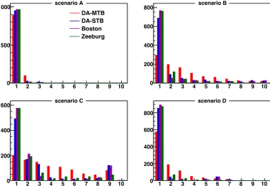
Figure 2 shows the distribution of the assigned rank for one single experiment for each of the four scenarios. The first bin shows how many students get assigned to the school of their first choice, the second bin their second choice, etc. These distributions will look different for every experiment, because the preferences of the students differ and because the tie-breakers used in the matching algorithms differ.
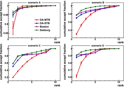
A convenient way to summarise the information in Fig. 2 for many experiments is to integrate this distribution, normalize it and average over the experiments. The result of this is shown in Fig 3. The curves in this figure show which fraction of students get assigned to the school of their first choice, to their first or second choice, etc.
It is clear from these graphs that independent of the scenario, the Boston algorithms assigns most pupils to the school of their first choice. This is a property of the algorithm: it actually assigns the maximum possible number of students to their first choice. The DA-MTB scores poorly when it comes to the first choice, but it has a smaller tail. The reason for this is that with multiple tie-breakers, it is unlikely that a student is unlucky at every school.
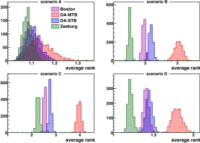
Each of the points in Fig. 3 has a vertical ‘error’ bar. The size of the error reflects the variation in the integrals between the different experiments. This variation is larger for the DA-MTB algorithms than for the Boston algorithm, because the former is more sensitive to the random numbers in the tie-breaker. Another way to represent the variation between experiments is to consider the distribution of the average rank (our qualifier Q) in each experiment, shown in Fig. 4. In scenario A the difference between the algorithms is small, but in all others it is substantial. In terms of the qualifier defined above, there is clear order in the efficiency of the four algorithms, with Zeeburg having the highest efficiency
6
1 2 3 4 5 6 7 8 9 10 0
500 1000
DA-MTB DA-STB Boston Zeeburg scenario A
1 2 3 4 5 6 7 8 9 10
0 200 400 600
800 scenario B
1 2 3 4 5 6 7 8 9 10
0 200 400
600 scenario C
1 2 3 4 5 6 7 8 9 10
0 200 400 600 800
[image:8.595.106.499.73.352.2]scenario D
Figure 2: Distribution of rank for one experiment in each of the four scenarios sketched in the text for the Boston, DA-STB and DA-MTB algorithms. Each distribution has a thousand entries, corresponding to the thousand students in the experiment.
and DA-MTB the lowest. For example, in scenario B students are on average assigned to their third rank school by the DA-MTB algorithm, while the average assignment of Zeeburg is between the first and second ranked school.
Figure 4 also indicates a large variation in the rank of an algorithm between different experiments. This variation has two sources, namely the actual differences in the datasets and the random character of the tie-breakers. To illustrate the importance of the latter we show yet another distribution. For each experiment we run the algorithms a second time, but with a different tie-breaker, a different student lottery. For each algorithm we now count how many students are the second time assigned to a different school, that is, how ‘deterministic’ the algorithm is. The result is shown in Fig. 5 for all four algorithms. Comparing to Fig. 4 we note that that the sensitivity to the tie-breaker is correlated with the efficiency: the less important the tie-breaker, the more efficient the algorithm.
3.3. The pairwise exchange method
Given a particular set of matches one can improve the average ranking using
pairwise exchanges (PE), a swap of the schools assigned to a pair of students. In
principle, using pairwise exchanges one can transform any solution into any other, including the optimal solution. In practice, in order to limit the time-consumption of such an algorithm, it is necessary to limit the set of considered exchanges.
rank
0 5 10
cu mu lati ve accep t fract io n 0.85 0.9 0.95 1 DA-MTB DA-STB Boston Zeeburg scenario A rank
0 5 10
cu mu lati ve accep t fract io n 0.4 0.6 0.8 1 scenario B rank
0 5 10
cu mu lati ve accep t fract io n 0.2 0.4 0.6 0.8 1 scenario C rank
0 5 10
[image:9.595.94.501.69.356.2]cu mu lati ve accep t fract io n 0.6 0.7 0.8 0.9 1 scenario D
Figure 3: Average cumulative acceptance functions for the four considered scenarios and for the Boston, DA-STB and DA-MTB algorithms, averaged over 1000 experiments. The vertical error bars correspond to the standard deviation of the variation between experiments.
pairwise exchange method to be effective, such exchanges should be considered. Besides pairwise exchanges, one can also consider exchanges of higher order in which the average improves. Unfortunately, in our implementation in the python programming language, the time consumption of even a tripple exchange algorithm was found to be prohibitively large and we have not pursued this any further.
The pairwise exchange method may reduce the number of students assigned to their first preference. Although this is perfectly allowed, we do build in a small bias towards rank one: Besides exchanges that decrease the average rank, we also consider exchanges that leave the average rank invariant, but for which the minimum of the rank of the two students after the exchange is smaller than before. That is, we prefer an assignment with ranks one and three to an assignment with ranks two and two, etc.
Our pairwise exchange algorithm thus becomes:
1. order the pupils in decreasing rank according to the original solution; 2. starting from the first pupil, labeled i, consider an exchange with all other
pupils, labeled j;
3. if the change in the average rank is smaller than zero, or if it is equal to zero but the minimum of the ranks of the two students becomes smaller, make the exchange;
4. continue until exchanges of all pairs of pupils have been considered.
average rank
1 1.1 1.2 1.3 0
50 100 150
200 Boston
DA-MTB DA-STB Zeeburg scenario A
average rank
1 2 3
0 200 400
600 scenario B
average rank
1 2 3 4
0 200 400 600
scenario C
average rank
1 1.5 2
0 100 200 300
[image:10.595.106.500.74.356.2]scenario D
Figure 4: Distribution of the average rankQover 1000 experiments for the four different scenarios in the Boston, DA-STB, DA-MTB and Zeeburg algorithms.
more than once we have verified that the algoritm effectively converges in one iteration.
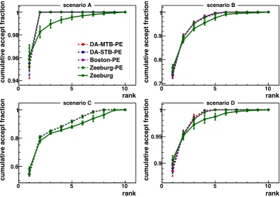
Figure 6 shows the cumulative acceptance functions for all four algorithms after the PE algorithm is applied. It is both interesting and reassuring that the curves depend little on which algorithm was used to provide the solution that the PE starts from. The PE algorithm can be successfully applied to improve the inefficiency of any of the tested algorithms to about the same level. This is also indicated by the average rank Q shown in Tab. 2 for all scenarios and for all algorithms before and after the pairwise exchange.
A B C D
[image:10.595.133.465.556.679.2]DA-MTB 1.14±0.05 3.03±0.13 3.96±0.09 1.79±0.06 DA-STB 1.11±0.03 2.17±0.06 2.76±0.05 1.45±0.04 Boston 1.10±0.03 1.95±0.05 2.53±0.04 1.41±0.03 Zeeburg 1.08±0.02 1.51±0.04 2.26±0.07 1.21±0.03 DA-MTB-PE 1.05±0.01 1.44±0.03 2.06±0.04 1.18±0.02 DA-STB-PE 1.04±0.01 1.44±0.03 2.06±0.04 1.18±0.02 Boston-PE 1.04±0.01 1.43±0.03 2.06±0.04 1.17±0.02 Zeeburg-PE 1.04±0.01 1.43±0.03 2.07±0.04 1.17±0.02
Table 2: Average rankQfor the scenarios and algorithms discussed in the text for 1000 experi-ments. The quoted error is the standard deviation of the variation between experiexperi-ments.
number of changes
0 200 400 600 800 1000
0 100 200 300
400 DA-MTB
DA-STB Boston Zeeburg scenario A
number of changes
0 200 400 600 800 1000
0 100 200 300 400
scenario B
number of changes
0 200 400 600 800 1000
0 100 200 300 400
scenario C
number of changes
0 200 400 600 800 1000
0 200 400
[image:11.595.104.504.72.353.2]600 scenario D
Figure 5: Number of students that gets a different assignment in two consecutive calls to the same algorithm in 1000 experiments.
in the assignment. However, as illustrated in the right figure, the solutions are actually very close in rank. We found that most of the difference between the solution can be attributed to pairs of students that have exchanged places such that the final change is rank neutral, simply because the students have ranked the two schools in the same way.
One may wonder how close to the optimal solution the result of the pairwise exchange is. As the starting point is determined by the random tie-breaker and only a finite set of pairwise exchanges is tried, the result may correspond to a ‘local minimum’ of the average rank. As a different local minimum is obtained with a different tie-breaker, one can try to assess the distance to the true minimum by trying different random tie-breakers. We have compared the average rank obtained with a single call to Boston plus PE to that obtained with a pick of ‘the best of 10’. The difference was found to be small, of the order of the variations seen on the right in Fig. 7. We did not study the asymptotic behaviour in more detail but it seems that in practice the solution is close to optimal.
rank
0 5 10
cu mu lati ve accep t fract io n 0.94 0.96 0.98 1 DA-MTB-PE DA-STB-PE Boston-PE Zeeburg-PE Zeeburg scenario A rank
0 5 10
cu mu lati ve accep t fract io n 0.7 0.8 0.9 1 scenario B rank
0 5 10
cu mu lati ve accep t fract io n 0.6 0.8 1 scenario C rank
0 5 10
[image:12.595.94.501.70.356.2]cu mu lati ve accep t fract io n 0.9 0.95 1 scenario D
Figure 6: Average cumulative acceptance functions for a 1000 experiments in the four considered scenarions and for the DA-MTB, DA-STB, Boston and Zeeburg algorithm after the pairwise exchange (PE) algorithm. The Zeeburg algorithm without PE is included for the comparison. The vertical error bars correspond to the RMS of the variation between experiments.
3.4. Tests of strategy-proofness
A matching method is strategy-proof if pupils do not benefit from specifying a preference list different from their true ordinal preference. It is not apriori clear what ‘benefit’ means in this context, since there is always a price to pay. As we shall see below, students could apply a strategy that gives them a higher chance to get their first preference, at the expense of having a higher change to end up with a school that ranks low on their list; or they could aim to increase the chance to get within their top three, by ranking their actual first choice lower. Therefore, one may argue that determining a strategy is just a cost-benefit analysis that individual pupils should be allowed to make.
The main reason that we should worry about strategy-proofness anyway is because pupils that do not apply a strategy may be harmed by the behaviour of the strategists. This leads to a form of inequality as the background of students and parents influences their ability to understand the consequences of different strategies. In the following we test the effect of two simple selection strategies in our simulations.
It should be emphasised that for a subset of students the current system in Amsterdam is already not strategy-proof for any matching algorithm. The reason is that some schools give preference to students that either have brothers or sisters at the same school, or that attended a certain type of primary school. As this preference is only given if students rank the school first, it is an incentive to put the school at the first place, even if it is not actually the first preference.
number of changes
0 200 400 600 800 1000
0 200 400
DA-STB-PE Boston-PE Zeeburg-PE Zeeburg scenario C
Q Δ 0.1
−0 −0.05 0 0.05 0.1
100 200 300
[image:13.595.106.505.72.216.2]scenario C
Figure 7: Distributions for the number of students changing school (left) and the change in the average rank (right) after two consecutive calls to the algorithm in scenario C for 1000 experiments.
rank
0 5 10
cu
mu
lati
ve
accep
t
fracti
o
n
0.7 0.8 0.9 1
Boston-PE Boston-PEM scenario B
rank
0 5 10
cu
mu
lati
ve
accep
t
fracti
o
n
0.6 0.8 1
Boston-PE Boston-PEM scenario C
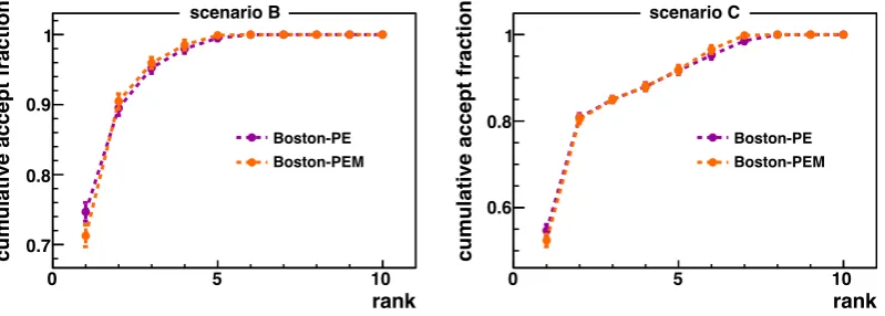
Figure 8: Average cumulative acceptance functions for a 1000 experiments in scenario B and C for Boston with the default pairwise exchange algorithm (PE) and for pairwise exchange with minimal variance (PEM).
algorithms for students that apply different kind of strategies. We have found that, in practice, it is not that simple to define a popularity scenario and a ranking strategy that actually lead to a benefit for strategic students. After some trial and error, we have come up with scenario C: two schools that are so popular that mosts student will rank them as one and two, and two schools that are so unpopular that they are almost always at the bottom of the list.
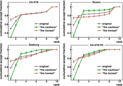
In this scenario strategic students can try to evade the unpopular school by putting one of the less unfavourable schools in their top two. To keep the imple-mentation generic the actual applied strategy is that students re-order their true top three according to the known average popularity (table 1). Figure 9 shows the effect on the acceptance curves in a simulation of scenario C with 50% of the students applying this strategy. Note that the cumulative acceptance is given as function of the true rank, not the rank that the strategic student provided. The students applying a strategy are called ‘cautious’, while the remaining students in the sample are ‘honest’. For reference also the original curves with only honest students are shown.
[image:13.595.100.500.276.419.2]rank
2 4 6 8 10
cu mu lati ve accep t fract io n 0.4 0.6 0.8 1 original "the cautious" "the honest" DA-STB rank
2 4 6 8 10
cu mu lati ve accep t fract io n 0.4 0.6 0.8 1 original "the cautious" "the honest" Boston rank
2 4 6 8 10
cu mu lati ve accep t fract io n 0.4 0.6 0.8 1 original "the cautious" "the honest" Zeeburg rank
2 4 6 8 10
[image:14.595.94.502.70.355.2]cu mu lati ve accep t fract io n 0.4 0.6 0.8 1 original "the cautious" "the honest" DA-STB-PE
Figure 9: Average cumulative acceptance as function of thetrue rank with and without 50% of the students following the ‘cautious’ strategy described in the text for 100 experiments according to popularity scenario C.
not strategy-proof in this scenario: although the cautious loose on their top one and two ranking, they beat their victims in the top three and beyond. The Zeeburg algorithm and any algorithm combined with pairwise-exchange optimisation are not strategy-proof either. Interesting enough, in this scenario, they seem to be more strategy-proof than Boston, even though they are more efficient. This shows that efficiency is not directly coupled to strategy-proofness.
In any case, it is important to note that in this scenario the victims are not worse off with any of the improved algorithms than they are with DA-STB. This can be seen by comparing the ‘original’ curve for DA-STB with the ‘honest’ curve in DA-STB-PE. The costs of DA’s strategy-proofness is simply too high to com-pensate for the inefficiency caused by the lack of strategy-proofness in the other algorithms.
rank
2 4 6 8 10
cu
mu
lati
ve
accep
t
fract
io
n
0.4 0.6 0.8 1
original "the gamblers" "the honest" Zeeburg
rank
2 4 6 8 10
cu
mu
lati
ve
accep
t
fract
io
n
0.4 0.6 0.8 1
[image:15.595.95.503.72.215.2]original "the gamblers" "the honest" DA-STB-PE
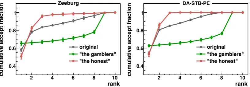
Figure 10: Average cumulative acceptance as function of thetrue rank with and without 50% of the students following the ‘gambling’ strategy described in the text for 100 experiments according to popularity scenario C.
[image:15.595.156.439.271.369.2]cautious gambling strategists honest strategists honest Boston 2.50 2.73 3.68 1.66 Zeeburg 2.26 2.20 3.41 1.79 Boston-PE 2.33 2.00 3.58 1.61 Zeeburg-PE 2.31 2.03 3.55 1.63 DA-STB-PE 2.34 1.99 3.58 1.61
Table 3: Average (true) rank Qfor strategic and honest pupils measured over 100 experiments in scenario C with either 50% cautious strategists (left) or 50% gambling strategists (right).
Table 3 shows the average rank obtained for strategic and honest pupils in the scenarios above. One clearly observes the price the strategists pay: as they do not provide their true preferences, their average rank is usually higher than for the honest students. Comparing to Tab. 2 we find that in terms of the average rank the honest do not score worse in Zeeburg and PE algorithms than they did without the strategists.
In the other scenarios (A, B and D) the negative effect on honest students as a result of cautious and gambling strategies was found to be insignificant. That does not mean that there do not exist scenarios in which honest students are better off with a strategy-proof inefficient algorithm as DA-STB. However, it illustrates that in practice such scenarios may be rare.
4. Practical considerations and other discussion points
4.1. School preferences
Some of the schools in Amsterdam may give a subset of pupils a preference over others, for example because elder siblings attend the school. In order to respect these constraints, they need to be built into the tie-breaker at the school. It is not easy to use such constraint in the Zeeburg algorithm. The easiest solution is to deal with this subset of students first, and use the matching algorithms only for the students that remain.
4.2. Incomplete preference lists
they may hand in a list with just one school. If a pupil cannot be assigned to that school in Boston or DA, the consequence is that the pupil needs to participate in a second round, in which only schools participate that still have places left.
Clearly, this has consequences for the implementation of the algorithms. For instance, the Zeeburg and pairwise exchange cannot be applied in a fair way unless all preference lists are complete, as students may on purpose hand in lists that do not contain less popular schools.
One practical solution is to complete the preference lists. They could be com-pleted deterministically as follows: once the preference lists are available, schools are ranked by popularity. Every pupil preference lists is completed with the miss-ing schools in order of increasmiss-ing popularity. This is a clear motivation for students to hand in a long preference list.
4.3. School types
In contrast to many other countries in the world, the school system in the Netherlands differentiates the level of education directly at the start of secondary education. The level appropriate for a pupil’s secondary education is determined by the teachers at the primary school based on scores to standard tests performed during the pupil’s primary school career. The proposed level is called the advice.
There are roughly four ‘levels’ of education. In theory, this just splits the matching in four independent parts. In practice, it is not that simple. First, students may be given a mixed advice. Second, many schools offer transition classes for the first or second year that combine more than one level.
This complication is not a show-stopper, however. If the matching can be applied with Boston or DA, then the pairwise exchange algorithm can be applied a such, as long as it only exchanges students that have the same school advice.
4.4. Simplicity
An important property of a suitable matching algorithm is that it is sufficiently simple that it can be both easily be explained and unambiguously described and implemented. In this respect the Zeeburg algorithm is perhaps a bordercase. How-ever, the pairwise exchange algorithm certainly qualifies as simple.
4.5. Alternative optimisation criterion
The pairwise exchange method optimised the average rank Q. In the optimi-sation the difference between rank 8 and 9 is the same as between rank 1 and 2. However, pupils probably care less about the order in the tail, than the order of their top ranked schools. This was the main reason that we preferred the PE method with larger variance over the one with minimal variance (PEM).
Still, one may wonder if alternative definitions of Q, for example as a power-law Q ∝ Pirα
i with α < 1, would not lead to a solution that better reflects the cardinal preferences of the pupils. Inevitably, this will lead to a larger tail in the rank distribution. We have not further investigated this.
5. Conclusions
both sides. The Boston algorithm better respects the students preferences. Other algorithms, such as the Zeeburg algorithm and the pairwise exchange optimisa-tion introduced here, perform even better, in a variety of simple scenarios. The reason is that the sensitivity to the tie-breaker, the lottery tickets of the pupils, is significantly smaller in these alternatives.
The inefficiency of the DA algorithms with random tie-breakers is the cost of strategy-proofness [4]. The more efficient algorithms are not strategy-proof. However, in the considered scenarios the costs of the lack of strategy-proofness is smaller than the costs of the inefficiency of DA: Even students that do not apply a strategy are better of with the non-strategy-proof algorithms. Therefore, it seems hard to maintain strategy-proofness as a requirement of the matching algorithm.
To understand whether or not these conclusions hold in more realistic scenarios, an analysis like the one in [8] will need to be performed. However, based on the current results we strongly advise local authorities to reconsider their choice for DA in school matching. The most simple way to ‘fix’ the algorithm is to augment it with the pairwise exchange algorithm that we described. This algorithm is simple and suffers little from the practical limitations discussed above. We believe that by applying this method, the results of the matching will be significantly more in line with the students preferences.
From personel experience we know that pupils and their parents spend a lot of effort to prioritise the schools in Amsterdam. If these efforts are taken seriously, random number should play a minimal role in the matching.
6. Acknowledgements
The author would like to thank Dr. Paola Grosso, Dr. Edward Hulsbergen, Rola Hulsbergen-Paanakker, Prof. Dr. Olga Igonkina, Prof. Dr. Gerhard Raven, Hartmut Samtleben and Dr. Wouter Verkerke, for stimulating discussions and corrections to this write-up.
Appendix A. The Zeeburg algorithm
The DA and Boston algorithms rely on a random tie-breaker that effectively describes the school preferences. We have implemented another algorithm in which the number of ties broken by the random tie-breaker is minimised. The algorithm works as follows:
1. For every school keep track of
(i.) the number of vacant places at the school; (ii.) the rank of the current queue;
(iii.) the pupils in the queue.
In addition keep track of the list of completed student-school matches. This defines the state of the algorithm.
2. Sort pupils according to a single random tie-breaker. Set the rank of the queue of every school to one and assign the number of vacant places. Line up pupils in the queue of their favourite school. This populates the queue in every school and completes theinitial state of the algorithm;
(a.) select a school that can entirely admit the queue of its current rank. If there is more than one such school, select the school with the queue with the smallest rank. If there is more than one such queue, select the school for which the number of places remaining after accepting all pupils in the queue is the smallest;
(b.) for this queue, accept all pupils. Remove these pupils in every other queue that they appear. (Initially, pupils appear in only one queue, but this changes while the algorithm is running.) Reduce the number of vacant places according to the number of newly accepted students. If there are places left at the school, increase the rank of the queue, and line up all pupils that have not yet found a place and that rank the school according to the rank of the queue. (These students will now be in more than one queue);
(c.) repeat until the condition under (3a.) can no longer be satisfied for any school.
4. Apply the tie-breaker to force a decision on one of the queues:
(a.) select the queue with the smallest rank in a school that is not yet full. If there is more than one such queue, select the queue that has the smallest overflow (that is, for which the length of the queue minus the number of available places is minimal);
(b.) accept pupils from the start of this queue until the school is full. Remove accepted pupils from other queues;
5. Repeat steps 3 and 4 until all pupils have been accepted.
References
[1] A. E. Roth, M. Sotomayor, The College Admissions Problem Revisited, Econo-metrica 57 (3) (1989) 559–570.
URL http://www.jstor.org/stable/1911052
[2] A. E. Roth, Deferred Acceptance Algorithms: History, Theory, Practice, and Open Questions, Working Paper 13225, National Bureau of Economic Research (July 2007). doi:10.3386/w13225.
URL http://www.nber.org/papers/w13225
[3] A. Abdulkadiro˘glu, T. S¨onmez, School Choice: A Mechanism Design Approach, The American Economic Review 93 (3) (2003) 729–747.
URL http://www.jstor.org/stable/3132114
[4] A. Abdulkadiro˘glu, P. A. Pathak, A. E. Roth, Strategy-proofness versus Effi-ciency in Matching with Indifferences: Redesigning the New York City High School Match, Working Paper 14864, National Bureau of Economic Research (April 2009). doi:10.3386/w14864.
URL http://www.nber.org/papers/w14864
[5] A. Abdulkadiro˘glu, Y.-K. Che, Y. Yasuda, Resolving Conflicting Preferences in School Choice: The “Boston Mechanism” Reconsidered, The American Eco-nomic Review 101 (1) (2011) 399–410.
[6] D. Gale, L. S. Shapley, College Admissions and the Stability of Marriage, The American Mathematical Monthly 69 (1) (1962) 9–15.
URL http://www.jstor.org/stable/2312726
[7] L. E. Dubins, D. A. Freedman, Machiavelli and the Gale-Shapley Algorithm, The American Mathematical Monthly 88 (7) (1981) 485–494.
URL http://www.jstor.org/stable/2321753
[8] M. de Haan, P. A. Gautier, H. Oosterbeek, B. van der Klaauw, The perfor-mance of school assignment mechanisms in practice, CESifo Area Conference on the Economics of Education, 2015.
URL http://www.cesifo-group.de/dms/ifodoc/docs/Akad_Conf/CFP_