Evaluation of Interdiffusion in Liquid Phase during Reactive Diffusion between Cu and Al

Evaluation of Interdiffusion in Liquid Phase during Reactive

Diffusion between Cu and Al

Yasuhiko Tanaka

and Masanori Kajihara

Graduate School, Tokyo Institute of Technology, Yokohama 226-8502, Japan

2_{Department of Materials Science and Engineering, Tokyo Institute of Technology}

Using Cu/Al diffusion couples initially composed of pure Cu and Al, the reactive diffusion in the binary Cu–Al system was experimentally examined in a previous study. The diffusion couple was isothermally annealed in the temperature range ofT¼973{1073K. Due to annealing, compound layers of the,and"phases are formed between the Cu-rich solid () phase and the Al-rich liquid (L) phase, and theL="interface migrates towards the"phase. At each annealing time, the migration distance of theL="interface is much greater than the total thickness of the compound layers. Furthermore, there exists the parabolic relationship between the migration distance and the annealing time. This means that the migration of the interface is controlled by the volume diffusion in theLphase. The mathematical model for the interface migration controlled by volume diffusion was used in order to analyze quantitatively the migration rate of the interface. Through the analysis, the interdiffusion coefficientDof theLphase was evaluated to be1:24109_,2:91109_and3:62109_m2_{/s atT¼973, 1023 and 1073 K, respectively.} Expressing the temperature dependence ofDasD¼D0expðQ=RTÞ, values ofD0¼1:42104m2/s andQ¼93:5kJ/mol were obtained by the least-squares method. According to the analysis, the interdiffusion coefficient is much greater for theLphase than for the solid phases. Consequently, theL="interface migrates towards the"phase, and the migration rate of the interface is much greater than the overall growth rate of the compound layers. [doi:10.2320/matertrans.47.2480]

(Received June 19, 2006; Accepted August 21, 2006; Published October 15, 2006)

Keywords: intermetallic compounds, bulk diffusion, analytical methods, reactive diffusion, kinetics

1. Introduction

There are many binary alloy systems where intermetallic compounds appear as stable phases.1)Reactive diffusion has been experimentally studied for such alloy systems by many investigators.2–31) _{In those experiments, diffusion couples}

were prepared from different pure metals or alloys and then isothermally annealed at appropriate temperatures. After annealing, some of the stable compounds were observed as layers at the interface in the diffusion couple. When the reactive diffusion is controlled by volume diffusion, the total thicknesslof the compound layers is expressed as a function of the annealing timetby the parabolic relationshipl2_¼Kt. Here,K is the parabolic coefficient. The parabolic relation-ship may be believed to hold good in many alloy systems. However, the volume diffusion is not necessarily the rate-controlling process of reactive diffusion for all the alloy systems.

The reactive diffusion in the binary Au–Sn system was experimentally observed using Sn/Au/Sn diffusion couples in previous studies.15–17) _{The diffusion couple was}

isother-mally annealed at temperatures betweenT ¼393and 473 K. Due to annealing, compound layers composed of AuSn, AuSn2and AuSn4are produced at the Au/Sn interface in the diffusion couple. The total thickness of the compound layers is proportional to a power function of the annealing time, and the exponent of the power function is 0.48, 0.42 and 0.36 atT ¼393, 433 and 473 K, respectively. Consequently, the exponent is smaller than 0.5 at most of the annealing temperatures, and thus the parabolic relationship does not hold good for the reactive diffusion in the binary Au–Sn system. This means that grain boundary diffusion as well as volume diffusion contributes to the rate-controlling process

and grain growth occurs at certain rates in the compound layers. Such a mixed rate-controlling process was recognized also for the reactive diffusion in the binary Ag–Sn,18)Ni– Sn19)and Cu–Sn20)systems.

For the binary Fe–Al system, the reactive diffusion was experimentally observed using Al/Fe/Al diffusion couples in a previous study.21) _{Owing to isothermal annealing atT ¼}

823{913K, a single compound layer of Fe2Al5is formed at the interface in the diffusion couple, and grows according to the parabolic relationship. This indicates that the growth of the Fe2Al5layer is controlled by volume diffusion. This type of rate-controlling process was observed also for the binary Pd–Sn system.22)_{In this case, compound layers consisting of}

PdSn4, PdSn3and PdSn2are formed atT ¼433K, but those composed of only PdSn4and PdSn3are produced atT ¼453

and 473 K. At all these temperatures, there exists the parabolic relationship between the total thickness of the Pd–Sn compound layers and the annealing time. As pre-viously mentioned, however, the parabolic relationship does not hold good for the binary Au–Sn, Ag–Sn, Cu–Sn and Ni–Sn systems. Therefore, the rate-controlling process of reactive diffusion varies depending on the alloy system.

The kinetics of the reactive diffusion controlled by volume diffusion was theoretically analyzed using a mathematical model in a previous study.32) _{In the theoretical analysis, a}

hypothetical binary alloy system composed of two primary solid solution phases and one intermetallic compound was considered in order to evaluate the growth rate of the compound in various semi-infinite diffusion couples initially consisting of the two primary solid solution phases with different solubility ranges and interdiffusion coefficients. The mathematical model was also used to analyze numerically the relationship between the temperature dependence of the interdiffusion in each phase and the kinetics of the reactive diffusion.33–35) As mentioned earlier, the single compound

layer of Fe2Al5 is formed during reactive diffusion in the binary Fe–Al system.21) _{Furthermore, the growth of the}

Fe2Al5 layer is controlled by volume diffusion. Thus, the mathematical model32)_{was used to analyze numerically the}

growth behavior of the Fe2Al5 layer in a previous study.36) Through the analysis, the interdiffusion coefficient of Fe2Al5 was evaluated quantitatively.

Recently, the reactive diffusion in the binary Cu–Al system was experimentally observed using Cu/Al diffusion couples by the present authors.28) _{In that experiment, the}

diffusion couple was isothermally annealed in the temper-ature range betweenT ¼973and 1073 K. In this temperature range, Cu is solid, but Al is liquid. During annealing, compound layers composed of the , and " phases are formed at the interface between the Cu-rich solid () phase and the Al-rich liquid (L) phase. The total thicknesslof the compound layers is proportional to a power function of the annealing timet, and the exponent of the power function is 0.15, 0.41 and 0.33 at T¼973, 1023 and 1073 K, respec-tively. Hence, the exponent is smaller than 0.5 at all the annealing temperatures. As a consequence, like the binary Au–Sn,15–17)_Ag–Sn,18)_Ni–Sn19)_{and Cu–Sn}20)_{systems, grain}

boundary diffusion as well as volume diffusion contributes to the rate-controlling process and grain growth takes place at certain rates in the compound layers for the binary Cu–Al system. Unfortunately, however, the mathematical model32) mentioned above cannot be applicable to such a rate-controlling process. On the other hand, the interface between the L and " phases migrates towards the " phase during reactive diffusion in the binary Cu–Al system. Furthermore, the migration distancewof theL="interface is much greater than the total thickness l of the compound layers, and the square of the migration distance w is proportional to the annealing timet. This means that interdiffusion occurs more remarkably in theLphase than in the,,and"phases, and the migration of theL="interface is controlled by the volume diffusion in theLphase. In the present study, the interdiffu-sion coefficientDfor volume diffusion in theLphase of the binary Cu–Al system was quantitatively evaluated from the experimental result for the migration behavior of the L=" interface.

2. Experimental Summary

As mentioned in Section 1, the reactive diffusion in the binary Cu–Al system was experimentally observed in a previous study.28) _{In that experiment, columnar diffusion}

couples consisting of pure solid Cu and pure liquid Al were isothermally annealed in the temperature range betweenT¼

973and 1073 K. Here, the diameter is 8 and 8.5 mm for Cu and Al, respectively, and the initial thickness is 5 and 4.8 mm for Cu and Al, respectively. The interface between Cu and Al is flat and perpendicular to the columnar axis. During annealing, compound layers of the , and " phases are produced at the interface in the Cu/Al diffusion couple. According to a recent phase diagram in the binary Cu–Al system,37) the , and " phases are the only stable compounds atT ¼973{1073K. At these temperatures, the and"phases are in equilibrium with the Cu-rich solid () and Al-rich liquid (L) phases, respectively. Consequently, all

the stable phases were recognized in the annealed Cu/Al diffusion couple. The layer composed of the,and"phases is hereafter called the intermetallic layer. The total thicknessl

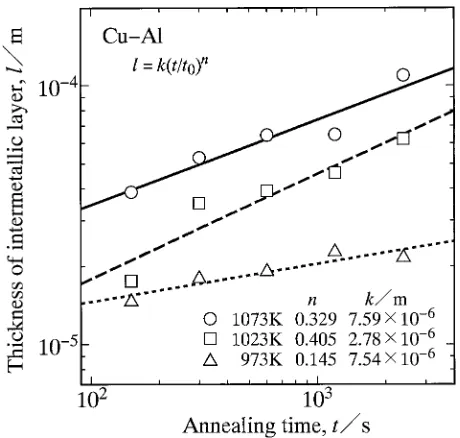
of the intermetallic layer was determined experimentally. The values of l are plotted against the annealing time t in Fig. 1. In this figure, the ordinate and the abscissa show the logarithms of l and t, respectively. Furthermore, open triangles, squares and circles indicate the results ofT ¼973, 1023 and 1073 K, respectively. As can be seen, the thicknessl

monotonically increases with increasing annealing time t. The plotted points at each annealing temperature are located well on a straight line. This yields that the thickness l is expressed as a power function of the annealing timetby the equation

l¼kðt=t0Þn: ð1Þ

Here,t0is unit time, 1 s. It is adopted to make the argument

t=t0of the power function dimensionless. The proportionality coefficientkhas the same dimension as the thickness l, but the exponent nis dimensionless. From the plotted points in Fig. 1, the values ofkandn were determined by the least-squares method. The determined values are shown in Fig. 1. Using these values ofkandn, the thicknesslwas calculated as a function of the annealing timetfrom eq. (1). The results ofT ¼973, 1023 and 1073 K are indicated as dotted, dashed and solid lines, respectively, in Fig. 1. At each experimental annealing time, the thicknesslmonotonically increases with increasing annealing temperature T. Thus, the higher the annealing temperatureT is, the faster the intermetallic layer grows.

along grain boundaries with a finite thickness in the intermetallic layer at annealing temperatures where the volume diffusion is much slower than the grain boundary diffusion. When grain growth occurs in the intermetallic layer, the volume fraction of the grain boundaries monotoni-cally decreases with increasing annealing time. Such de-crease in the volume fraction causes the decrement of the effective cross-section, and decelerates the grain boundary diffusion. As a result,n becomes smaller than 0.5.38)_When

the grain growth occurs very sluggishly, the volume fraction of the grain boundaries remains almost constant during annealing. In such a case, the effective cross-section for the grain boundary diffusion hardly varies, and thusnis almost equal to 0.5. According to the result in Fig. 1,n is smaller than 0.5 at all the annealing temperatures. Consequently, it is concluded that the grain boundary diffusion as well as the volume diffusion contributes to the rate-controlling process and the grain growth occurs at certain rates in the inter-metallic layer for the reactive diffusion in the binary Cu–Al system atT¼973{1073K.

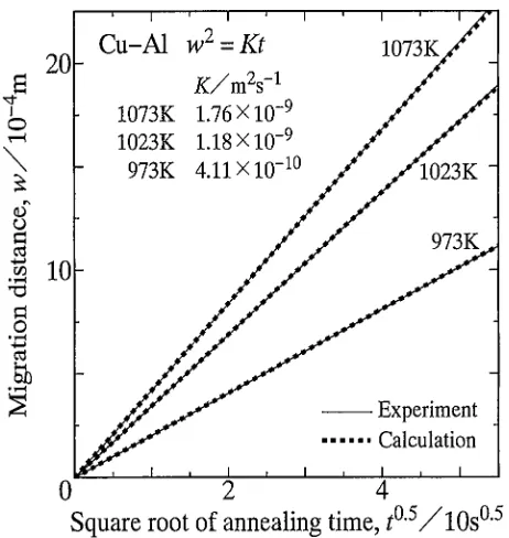
During growth of the intermetallic layer, the interface between the L and " phases migrates towards the" phase. Subtracting the thicknesses of the intermetallic layer and the phase from the initial thickness of the phase, we can determine the migration distance wof the L=" interface at each annealing time.28)The values ofw are plotted against the annealing time t in Fig. 2. In this figure, the ordinate indicates the migration distance w, and the abscissa shows the square root of the annealing time t. Open triangles, squares and circles indicate the results ofT ¼973, 1023 and 1073 K, respectively. Although the open triangles are rather scattered, most of the plotted points lie well on the corresponding straight line. This means that the parabolic relationship holds good betweenwandtas follows.

w2¼Kt ð2Þ

Here,Kis the parabolic coefficient with a dimension of m2/s. From the plotted points in Fig. 2, the value of K was evaluated at each annealing temperature by the least-squares method. The evaluated values of K are shown in Fig. 2. Using these values ofK,wwas calculated as a function of

tfrom eq. (2). The results ofT ¼973, 1023 and 1073 K are indicated as dotted, dashed and solid lines, respectively, in Fig. 2.

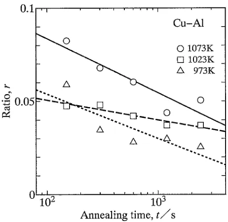
The ratiorof the thicknesslto the migration distancewis defined as

r¼l=w: ð3Þ

The values ofr are plotted against the annealing time t in Fig. 3. In this figure, the ordinate shows the ratior, and the abscissa indicates the logarithm of the annealing timet. Open triangles, squares and circles show the results of T ¼973, 1023 and 1073 K, respectively. As can be seen, the ratio

r takes values between 0.03 and 0.08 under the present annealing conditions. Although the plotted points are slightly scattered in Fig. 3, various straight lines indicate thatris a monotonically decreasing function of t. Consequently, we may conclude that the thicknessl is much smaller than the migration distanceweven at longer annealing times.

The values ofK are plotted against the annealing temper-atureT as open circles in Fig. 4. In this figure, the ordinate shows the logarithm of K, and the abscissa indicates the reciprocal of T. If the temperature dependence of K is expressed by the equation

K¼K0expðQK=RTÞ; ð4Þ

the pre-exponential factorK0and the activation enthalpyQK are evaluated to be 3:01103_m2_{/s and 127 kJ/mol,} respectively, from the open circles in Fig. 4 by the least-squares method. Here, R is the gas constant. Using these parameters,Kwas calculated as a function ofTfrom eq. (4). The result is shown as a solid line in Fig. 4.

Fig. 2 The migration distancewof theL="interface versus the square root of the annealing timet shown as open triangles, squares and circles at

T¼973, 1023 and 1073 K, respectively. Straight lines indicate the calculations from eq. (2).

3. Model

As mentioned in Section 2, the thickness l of the intermetallic layer is much smaller than the migration distance wof theL="interface. This means that interdiffu-sion occurs less remarkably in the,, and"phases than in the L phase. In such a case, the migration rate of the

L="interface is predominantly determined by the interdiffu-sion in theL phase, and thus can be described by a simple mathematical model. This model will be explained briefly below.

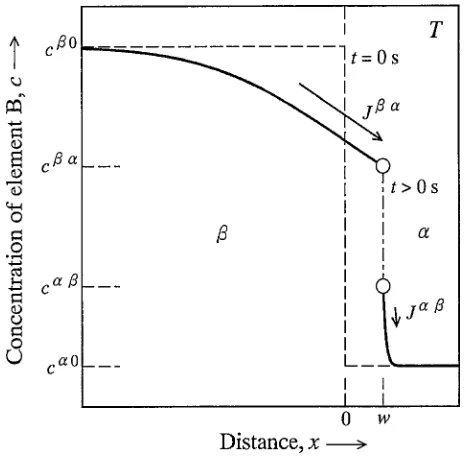
Let us consider a semi-infinite diffusion couple composed of theandphases with initial compositions ofc0_andc0_, respectively. Here, theandphases are the A-rich and B-rich phases, respectively, in a binary A–B system, andcis the concentration of element B measured in mol per unit volume. In the infinite diffusion couple, the thickness is semi-infinite for theandphases, and the=interface is flat. Therefore, the interdiffusion of elements A and B occurs unidirectionally along the direction perpendicular to the flat interface. This direction is called the diffusional direction. If the diffusion couple is annealed at temperature T for an appropriate time, the=interface will migrate towards the or phase depending on the flux balance at the interface. The concentration profile of element B along the diffusional direction across the = interface is schematically drawn in Fig. 5. In this figure, the ordinate shows the concentration

c, and the abscissa indicates the distance xmeasured from the initial position of the=interface. When the migration of the=interface is controlled by the volume diffusion in theandphases and the molar volumes of these phases are equivalent each other, the migration rate dw=dt of the interface is related to the flux balance at the interface by the equation39)

ðccÞdw

dt ¼J

_{J: ð5Þ}

Here, w is the migration distance of the = interface measured from the origin of the distancex,candcare the compositions of the and phases, respectively, at the interface, and J and J are the diffusional fluxes of element B due to the volume diffusion in theandphases, respectively, at the interface. According to Fick’s first law, the diffusional flux J _{is proportional to the concentration}

gradient@c_{=@xas follows.}

J¼ D@c

@x ð¼; Þ ð6Þ

In eq. (6),D_{is the interdiffusion coefficient for the volume}

diffusion in thephase, wherestands forand. When the interdiffusion coefficientD _{is independent of the}

com-position of the phase, Fick’s second law is expressed as follows.

@c @t ¼D

@

2_c

@x2 ð¼; Þ ð7Þ

Equation (7) shows that the compositionc is a function of the distancexand the annealing timet. For the semi-infinite =diffusion couple, the initial conditions are described as

cðx>0;t¼0Þ ¼c0 ð8aÞ

and

cðx<0;t¼0Þ ¼c0; ð8bÞ

and the boundary conditions are expressed by the equations

cðx¼w;t>0Þ ¼c; ð9aÞ

cðx¼w;t>0Þ ¼c; ð9bÞ

cðx¼ þ1;t>0Þ ¼c0 ð9cÞ

and

cðx¼ 1;t>0Þ ¼c0: ð9dÞ Fig. 4 The parabolic coefficientKversus the reciprocal of the annealing

temperatureTshown as open circles. The evaluations for the interdiffu-sion coefficientDof theLphase are indicated as open squares. Solid and

Under these initial and boundary conditions, eqs. (5)–(7) are solved analytically. If D _{is much smaller than D, J}

becomes negligible compared withJ_{according to eq. (6)}

unless@c_{=@xis much smaller than@c=@x. In such a case, the}

following equation is obtained from eqs. (5) and (6).

ðccÞdw

dt ¼J

¼ D@c

@x

x¼w

ð10Þ

For the migration of the = interface controlled by the volume diffusion, the migration distancewis expressed as a function of the annealing timetby the equation39)

w¼Kw ffiffiffiffiffiffiffiffiffiffi 4D_t

p

: ð11Þ

Here,Kwis the dimensionless coefficient. The coefficientKw is related with the initial and boundary conditions in eqs. (8) and (9) as follows.39)

expfðKwÞ2g

Kwf1þerfðKwÞg ¼c

_c0

c0_c ffiffiffi

p

ð12Þ

On the other hand, the following equation is obtained from eqs. (2) and (11).

w2 ¼4DðKwÞ2t¼Kt ð13Þ

Equation (13) shows that the parabolic coefficient K is expressed as a function of the interdiffusion coefficientDof the phase and the dimensionless coefficient Kw by the equation

K¼4DðKwÞ2: ð14Þ

SinceKw is dimensionless, the dimension ofK corresponds with that ofD_{according to eq. (14). Furthermore, K}

wis a function of c0_{,c andc}0 _{through eq. (12), and hence K} becomes a function ofc0_,c,c0_{andDvia eq. (14). Thus,}

D _{is an inverse function of c}0_{, c, c}0 _{and K.} Conse-quently,D_{can be evaluated from the value ofKdetermined}

experimentally for given values ofc0_,candc0_.

4. Results and Discussion

4.1 Evaluation of interdiffusion

In the mathematical model mentioned in Section 3, the composition is described with the concentrationcof element B measured in mol per unit volume. On the other hand, the mol fractionyof element B is practically used to express the composition of each phase. However, the mol fraction yis readily converted into the concentration cby the equation

c¼y=Vm. Here, Vm is the molar volume of the relevant

phase. When the molar volumeVmis constant independently

of the composition at each annealing temperature, the concentrationsc0_,candc0_{in eq. (12) are automatically} replaced with the mol fractionsy0_,yandy0_{, respectively.} Here, the superscript of the mol fractionypossesses the same meaning as the concentration c. In the schematic concen-tration profile of Fig. 5, the diffusional fluxJ_{is much greater}

in thephase than in thephase, and thus the=interface migrates towards the phase. Consequently, the Cu-rich and Al-rich L phases in the Cu/Al diffusion couple correspond to the and phases, respectively, for the mathematical model in Section 3. However, the Lphase is actually in equilibrium with the " phase at each annealing

temperature, and thus the liquidus composition corresponds to the mol fractionyL"_{of theLphase for theLþ"two-phase}

tie-line. As a result, we obtain the following equation.

ðyL"y0Þpffiffiffif1þerfðKwÞgKw

ðyL0yL"ÞexpfðKwÞ2g ¼0 ð15Þ

Here,y0 andyL0are the initial compositions of theandL

phases, respectively. From eq. (15), Kw is calculated for given values of y0, yL" and yL0. Since Kw is an implicit function ofy0_,yL"_andyL0_{, however, the calculation cannot} be carried out in an explicit manner. Therefore, Newton-Raphson’s method40)_{was used to calculate numerically the}

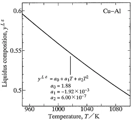
value of Kw from eq. (15). According to a recent phase diagram in the binary Cu–Al system,37) _yL"_{¼0:579, 0.542}

and 0.509 atT ¼973, 1023 and 1073 K, respectively. If the temperature dependence of the compositionyL"_{is described}

by the equation36)

yL"¼a0þa1Tþa2T2; ð16Þ

the following values are obtained:a0¼1:88,a1¼ 1:92

103 _{and a}

2¼6:00107. Using these parameters, the temperature dependence ofyL"_{was calculated from eq. (16).}

The result is shown as a solid curve in Fig. 6. Furthermore,

y0_{¼0 and y}L0_{¼1 for the Cu/Al diffusion couple. For} these values of y0_{, y}L" _{and y}L0_{, the calculation provides}

Kw¼0:288, 0.319 and 0.349 atT ¼973, 1023 and 1073 K, respectively. On the other hand, as shown in Fig. 2,

K¼4:111010,1:18109 and1:76109m2/s were experimentally determined at T ¼973, 1023 and 1073 K, respectively. Inserting these values ofKandKwinto eq. (14), we finally obtainD¼1:24109_,2:91109 _and3:62

109_m2_{/s atT¼973, 1023 and 1073 K, respectively, for the}

L phase in the binary Cu–Al system. The values of Dare plotted against the reciprocal ofT as open squares in Fig. 4. The temperature dependence ofDis usually described by the following equation of the same formula as eq. (4).

D¼D0expðQ=RTÞ ð17Þ

enthalpy. From the open squares in Fig. 4, D0¼1:42

104_m2_{/s andQ¼93:5kJ/mol are evaluated by the} least-squares method. Using these parameters,Dwas calculated as a function ofTfrom eq. (17). The result is shown as a dashed line in Fig. 4. As can be seen, the absolute value is slightly greater for D than for K at each annealing temperature. Sometimes, D may be roughly estimated from K by the equation

D¼ fK; ð18Þ

where f takes a constant value of 1, 0.5 or 0.25. This estimation insists thatDis not greater thanK. However,Dis greater thanK in Fig. 4, and thus f is greater than unity in eq. (18). Furthermore, Q is smaller than QK, and hence f varies depending on the temperature. Therefore, there is no adequate way to estimate the temperature dependence of f. Consequently, the interdiffusion coefficient D cannot be necessarily estimated only from the parabolic coefficientKin a straightforward manner.

The temperature dependence of the tracer diffusion coefficientD

i (i¼Cu, Al) is also expressed by the equation of the same formula as eq. (17) with the pre-exponential factor D

i0 and the activation enthalpy Qi. Unfortunately, however, reliable information is not available forD

Al0 and

Q

Alof the tracer diffusion coefficientDAlof Al in theLphase

of pure Cu. On the other hand, Ejima and co-workers41) determined values of D

Cu0¼1:0510

7_m2_{/s and Q}

Cu¼

23:8kJ/mol for the tracer diffusion coefficientD

Cuof Cu in

theLphase of pure Al. Using these values ofD_Cu0 andQ_Cu,

D_Cu was calculated as a function of the temperatureT from eq. (17). The result is shown as a dashed line in Fig. 7. In this figure, the ordinate indicates the logarithm of D

Cu, and the

abscissa shows the reciprocal ofT. The dashed line forDin Fig. 4 is indicated again as a solid line in Fig. 7. As can be seen,Dis close toD

Cu atT ¼973{1073K.

The solid-state reactive diffusion in the binary Cu–Al system was experimentally observed using Al/Cu/Al dif-fusion couples by Funamizu and Watanabe.42) _{In their}

experiment, the diffusion couple was isothermally annealed at temperatures betweenT¼673and 808 K. During anneal-ing, compound layers of the,,,andphases are formed at each interface in the diffusion couple. According to the observation, the parabolic relationship holds good between the mean thickness of each compound layer and the annealing time. This means that the growth of the compound layer is controlled by volume diffusion. From the exper-imental values of the parabolic coefficient at various annealing temperatures, the temperature dependence of the interdiffusion coefficient was estimated for each compound. The estimation gives D₀ ¼8:5105_m2_{/s and Q¼136}

kJ/mol as the pre-exponential factor and the activation enthalpy, respectively, of the interdiffusion coefficientDfor thephase.42)The temperature dependence ofD with these parameters is shown as a thin dashed line in Fig. 7. Since the and" phases are not stable atT ¼673{808K,37)_the

interdiffusion coefficient was not determined for these compounds in their experiment. On the other hand, the pre-exponential factor Ds

Al0 and the activation enthalpy QsAl of

the tracer diffusion coefficient Ds

Al of Al in pure Cu were

reported as follows: Ds

Al0¼1:31105m2/s and QsAl ¼

185kJ/mol.43)_{The temperature dependence ofD}s

Alwith these

parameters is shown as a thin dotted line in Fig. 7. As can be seen, bothDs

Al andD are much smaller thanD. Hence, we

may expect that the interdiffusion coefficient is much smaller also for the and " phases than for the L phase. Con-sequently, it is concluded that the diffusional flux is much smaller in the,,and"phases than in theLphase during reactive diffusion in the Cu/Al diffusion couple at T ¼

973{1073K. This is the reason why the L=" interface

migrates towards the" phase and the migration rate of the interface is much greater than the growth rates of the,and "layers.

4.2 Penetration depth of interdiffusion

At each annealing temperature, the mol fractionyof Al in theLphase is expressed as a function of the distancexand the annealing timetby the following equation.39)

y¼yL0þ y L"_yL0

1þerfðKwÞ

1þerf _{ffiffiffiffiffiffiffiffi}x 4Dt

p

; x<w ð19Þ

Here, xis measured from the initial position of the Cu/Al interface in the diffusion couple. From eq. (19), y was calculated as a function ofxfor the longest annealing time of

t¼2:4103_{s (40 min) using the following parameters as} well asyL0_{¼1and the value ofy}L"_{obtained from eq. (16):}

Kw¼0:288andD¼1:24109m2/s atT ¼973K;Kw¼ 0:319andD¼2:91109_m2_{/s atT ¼1023K; andK}

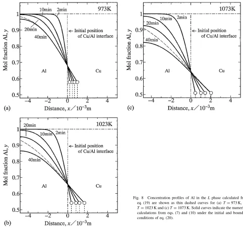
w¼ 0:349andD¼3:62109_m2_{/s atT ¼1073K. The results} of T ¼973, 1023 and 1073 K are shown as thin dashed curves in Fig. 8(a), (b) and (c), respectively. In this figure, the ordinate and the abscissa indicate the mol fractionyand the distancex, respectively. As long asyis equal toyL0_atx¼x

s,

the Cu/Al diffusion couple is considered semi-infinite during annealing. Here,xsis the position of the flat surface of theL

phase parallel to the interface. The initial thickness of theL

phase is 4.8 mm and the Lphase is initially located on the negative side ofxin Fig. 8, and thusxsis equal to4:8mm.

As can be seen in Fig. 8, however, the penetration depth of Fig. 7 Various diffusion coefficients versus the reciprocal of the

interdiffusion in the L phase exceeds the thickness of the

L phase at t¼2:4103s (40 min) for all the annealing temperatures, and hence y becomes smaller than yL0 at

x¼xs. Consequently, at the longest annealing time, the Cu/

Al diffusion couple is no longer semi-infinite. In such a case, eq. (19) is not applicable. In order to calculate the concen-tration profile in theLphase for various annealing times up to the longest time, eqs. (7) and (10) were solved numerically under the following initial and boundary conditions:

yLðx<0;t¼0Þ ¼yL0; ð20aÞ

yLðx¼w;t>0Þ ¼yL"; ð20bÞ

yðx¼w;t>0Þ ¼y0 ð20cÞ

and

@yL

@x

x¼xs

¼0: ð20dÞ

In the present numerical calculation, Crank-Nicolson implicit method44)was combined with a finite-difference technique.45) The results ofT ¼973, 1023 and 1073 K are shown as bold

solid curves in Fig. 8(a), (b) and (c), respectively. Open circles indicate the composition and the position of the interface at different annealing times. At T¼973K in Fig. 8(a), the penetration depth is smaller than the thickness of theLphase att¼1:2102and6:0102s (2 and 10 min) but greater than that of the L phase at t¼1:2103 _and

2:4103_{s (20 and 40 min). In contrast, at T ¼1023 and} 1073 K in Fig. 8(b) and (c), the penetration depth outstrips the thickness of theLphase even att¼6:0102_{s (10 min).} The annealing time dependence of the mol fraction ys at

x¼xswas deduced from the numerical calculation in Fig. 8.

The results of T¼973, 1023 and 1073 K are shown as dotted, dashed and solid curves, respectively, in Fig. 9. In this figure, the ordinate indicates the mol fractionys, and the

abscissa shows the square root of the annealing timet. As can be seen, ys is equal to yL0 at short annealing times. In this

case, the Cu/Al diffusion couple is considered semi-infinite. At long annealing times, however,ys becomes smaller than

yL0, and hence the diffusion couple is no longer semi-infinite. If the Cu/Al diffusion couple is not semi-infinite, the Fig. 8 Concentration profiles of Al in theLphase calculated from eq. (19) are shown as thin dashed curves for (a) T¼973K, (b)

parabolic relationship may not hold good even for the migration of the interface controlled by volume diffusion. Nevertheless, most of the plotted points at each annealing temperature are located well on the corresponding straight line in Fig. 2. The straight lines in Fig. 2 are indicated again as thin solid lines in Fig. 10. On the other hand, the relationship between the migration distance w and the annealing timetwas derived from the numerical calculation in Fig. 8. The results ofT ¼973, 1023 and 1073 K are shown as bold dotted curves in Fig. 10. As can be seen, the dotted curve coincides well with the solid line atT¼973K. Also

at T ¼1023 and 1073 K, the dotted curves mostly consist with the corresponding solid lines. As shown in Fig. 8(a), at

T ¼973K, the dashed curve agrees with the solid curve of

t¼2:4103_{s (40 min) except at small values ofx. Even at}

T ¼1023 and 1073 K, the dashed curves accord with the solid curves oft¼2:4103_{s (40 min) in the neighborhood} of the interface as indicated in Fig. 8(b) and (c), respec-tively. In Fig. 8, the dashed and solid curves show the concentration profiles for the semi-infinite and finite diffu-sion couples, respectively. According to eq. (10), the migra-tion rate of the interface is determined by the concentramigra-tion gradient in the L phase at the interface. As can be seen in Fig. 8, the concentration gradient at the interface is mostly equivalent for the semi-infinite and finite diffusion couples even at the longest annealing time. Therefore, almost the same migration rate of the interface is realized in both diffusion couples under the present annealing conditions. This is the reason why the parabolic relationship holds good within experimental uncertainty also at the long annealing times where the diffusion couple is no longer semi-infinite. When migration of an interface is controlled by volume diffusion in a semi-infinite diffusion couple, the migration surely obeys the parabolic relationship. However, the present numerical calculation indicates that the parabolic relation-ship holds good even for a finite diffusion couple as long as volume diffusion is the rate-controlling process and the penetration depth of interdiffusion merely slightly eclipses the thickness of each specimen in the diffusion couple.

5. Conclusions

The kinetics of the reactive diffusion in the binary Cu–Al system was experimentally observed in a previous study.28)

In that experiment, Cu/Al diffusion couples initially con-sisting of pure Cu and Al were isothermally annealed at temperatures ofT ¼973{1073K. At these temperatures, Cu is solid, but Al is liquid. During annealing, compound layers of the, and"phases37)_{are formed between the Cu-rich}

solid () phase and the Al-rich liquid (L) phase in the diffusion couple. Furthermore, the L=" interface migrates towards the"phase. Between the migration distancewof the

L=" interface and the annealing time t, there exists the parabolic relationship w2¼Kt, where K is the parabolic coefficient. The observation provides K¼4:111010,

1:18109 and 1:76109m2/s at T¼973, 1023 and 1073 K, respectively. The total thicknesslof the compound layers is much smaller than the migration distance w. This means that the migration of the L=" interface is predom-inantly controlled by the volume diffusion in theLphase. In order to evaluate the interdiffusion coefficient D of the L

phase, the experimental results were mathematically ana-lyzed using the diffusion equation describing the flux balance at the migrating interface.39) _{The analysis deduces D¼}

1:24109_,2:91109_and3:62109_m2_{/s atT ¼973,} 1023 and 1073 K, respectively. When the temperature dependence of D is expressed by the equation D¼

D0expðQ=RTÞ, values of D0¼1:42104m2/s and

Q¼93:5kJ/mol are obtained by the least-squares method. According to the analysis, the interdiffusion occurs much faster in the L phase than in the solid phases. This is the Fig. 9 The compositionysatx¼xsversus the square root of the annealing

timetfor the numerical calculation in Fig. 8 shown as dotted, dashed and solid curves atT¼973, 1023 and 1073 K, respectively.

reason why the L="interface migrates towards the "phase and the migration rate of the interface is much greater than the overall growth rate of the compound layers.

Acknowledgements

The present study was supported by a Grant-in-Aid for Scientific Research from the Ministry of Education, Culture, Sports, Science and Technology of Japan.

REFERENCES

1) T. B. Massalski, H. Okamoto, P. R. Subramanian and L. Kacprzak: Binary Alloy Phase Diagrams(ASM International, Materials Park, OH, 1990) vol. 1–3.

2) B. Lustman and R. F. Mehl: Trans. Met. Soc. AIME147(1942) 369– 394.

3) D. Horstmann: Stahl Eisen73(1953) 659–665.

4) S. Storchheim, J. L. Zambrow and H. H. Hausner: Trans. Met. Soc. AIME200(1954) 269–274.

5) G. V. Kidson and G. D. Miller: J. Nucl. Mater.12(1964) 61–69. 6) K. Shibata, S. Morozumi and S. Koda: J. Japan Inst. Met.30(1966)

382–388.

7) K. Hirano and Y. Ipposhi: J. Japan Inst. Met.32(1968) 815–821. 8) M. M. P. Janssen: Metall. Trans.4(1973) 1623–1633.

9) G. F. Bastin and G. D. Rieck: Metall. Trans.5(1974) 1817–1826. 10) M. Onishi and H. Fujibuchi: Trans. JIM16(1975) 539–547. 11) EI-B. Hannech and C. R. Hall: Mater. Sci. Tech.8(1992) 817–824. 12) P. T. Vianco, P. F. Hlava and A. L. Kilgo: J. Electron. Mater.23(1994)

583–594.

13) M. Watanabe, Z. Horita and M. Nemoto: Interface Science4(1997) 229–241.

14) S. Choi, T. R. Bieler, J. P. Lucas and K. N. Subramanian: J. Electron. Mater.28(1999) 1209–1215.

15) M. Kajihara, T. Yamada, K. Miura, N. Kurokawa and K. Sakamoto: Netsushori43(2003) 297–298.

16) T. Yamada, K. Miura, M. Kajihara, N. Kurokawa and K. Sakamoto: J. Mater. Sci.39(2004) 2327–2334.

17) T. Yamada, K. Miura, M. Kajihara, N. Kurokawa and K. Sakamoto: Mater. Sci. Eng. A390(2005) 118–126.

18) K. Suzuki, S. Kano, M. Kajihara, N. Kurokawa and K. Sakamoto:

Mater. Trans.46(2005) 969–973.

19) M. Mita, M. Kajihara, N. Kurokawa and K. Sakamoto: Mater. Sci. Eng. A403(2005) 269–275.

20) T. Takenaka, S. Kano, M. Kajihara, N. Kurokawa and K. Sakamoto: Mater. Sci. Eng. A396(2005) 115–123.

21) D. Naoi: Master Eng. Thesis, Tokyo Institute of Technology, 2006. 22) T. Takenaka, M. Kajihara, N. Kurokawa and K. Sakamoto: Mater. Sci.

Eng. A406(2005) 134–141.

23) T. Takenaka, S. Kano, M. Kajihara, N. Kurokawa and K. Sakamoto: Mater. Trans.46(2005) 1825–1832.

24) M. Mita, K. Miura, T. Takenaka, M. Kajihara, N. Kurokawa and K. Sakamoto: Mater. Sci. Eng. B126(2006) 37–43.

25) T. Takenaka and M. Kajihara: Mater. Trans.47(2006) 822–828. 26) T. Takenaka, M. Kajihara, N. Kurokawa and K. Sakamoto: Mater. Sci.

Eng. A427(2006) 210–222.

27) Y. Yato and M. Kajihara: Mater. Sci. Eng. A428(2006) 276–283. 28) Y. Tanaka, M. Kajihara and Y. Watanabe: Mater. Sci. Eng. A, in press. 29) Y. Yato and M. Kajihara: Mater. Trans.47(2006) 2277–2284. 30) Y. Muranishi and M. Kajihara: Mater. Sci. Eng. A404(2005) 33–41. 31) T. Hayase and M. Kajihara: Mater. Sci. Eng. A433(2006) 83–89. 32) M. Kajihara: Acta Mater.52(2004) 1193–1200.

33) M. Kajihara: Mater. Sci. Eng. A403(2005) 234–240. 34) M. Kajihara: Mater. Trans.46(2005) 2142–2149.

35) M. Kajihara: Defect and Diffusion Forum249(2006) 91–95. 36) M. Kajihara: Mater. Trans.47(2006) 1480–1484.

37) T. B. Massalski, H. Okamoto, P. R. Subramanian and L. Kacprzak: Binary Alloy Phase Diagrams(ASM International, Materials Park, OH, 1990) vol. 1, pp. 141–143.

38) Y. L. Corcoran, A. H. King, N. de Lanerolle and B. Kim: J. Electron. Mater.19(1990) 1177–1183.

39) W. Jost:Diffusion of Solids, Liquids, Gases (Academic Press, New York, 1960) pp. 68–82.

40) G. Dahlquist and A˚ . Bjo¨rck: Numerical Methods (Prentice-Hall, Englewood Cliffs, NJ, 1974) pp. 222–224.

41) T. Ejima, T. Yamamura, N. Uchida, Y. Matsuzaki and M. Nikaido: J. Jpn. Inst. Met.44(1980) 316–323.

42) Y. Funamizu and K. Watanabe: Trans. Jpn. Inst. Met.12(1971) 147– 152.

43) Metals Data Book, ed. Japan Institute of Metals (Maruzen, Tokyo, 1993) p. 21.

44) J. Crank:The Mathematics of Diffusion(Oxford Univ. Press, London, 1979) pp. 144–148.