Numerical Simulation of Shrinkage Formation of Pure Sn Casting Using Particle Method

Numerical Simulation of Shrinkage Formation

of Pure Sn Casting Using Particle Method

Naoya Hirata and Koichi Anzai

Department of Metallurgy, Graduate School of Engineering, Tohoku University, Sendai 980-8579, Japan

Shrinkage formation often causes fatal defects in castings. Recently, the development of computer technology has provided us with a useful and effective method to predict shrinkage formation. A particle method is a Lagrangian method that uses discrete objects as calculation elements which is referred to as particles, and they can move freely in the space. Therefore, this method can calculate shrinkage formation directly. In this study, solidification simulation and flow simulation programs based on the particle method were combined considering the temperature-dependency of density. The program was applied to the solidification problem of a cylindrical pure Sn casting, and the predicted shrinkage was compared with experimental results. First, the calculation stability for a still fluid was discussed and an improved method was proposed. The flow of a fluid during solidification is quite slow; however, the particle method has a fundamental difficulty in calculating slow flow phenomena. Therefore, creep flow was assumed. When the inertia force was not considered, the calculation stability improved significantly, and introduction of a gravity adjustment coefficient reduced calculation time significantly. Next, the proposed method was applied to shrinkage formation analysis with an influence of air-cooling. As a result, predicted shrinkage shape agreed well with experimental result.

[doi:10.2320/matertrans.M2011186]

(Received June 20, 2011; Accepted July 25, 2011; Published September 7, 2011)

Keywords: shrinkage formation behavior, solidification simulation, coupled simulation, particle method, moving particle semi-implicit (MPS) method

1. Introduction

Nowadays, computer simulation has acquired an important role in predicting casting defects. However, the conventional computer programs used for predicting casting defects have a fundamental limitation in calculating the combined effects of the various phenomena occurred during the casting process. Conventional computer programs are based on the Eulerian method that uses a calculation lattice, and the limitation is mainly due to the spatial constraint of the calculation lattice.1) In the calculation lattice, the calculation elements are sequentially arranged and the neighboring elements em-ployed in the interaction calculation are always the same; however, special methods are required to capture free surface. Therefore, the conventional computer programs are not suitable for calculating a large deformation such as shrinkage.

Recently, the fully Lagrangian method has attracted considerable attention. Particle methods based on Lagrangian methods involving no calculation lattice have been devel-oped rapidly because of their applicability to multi-physics problems.1) _{The SPH (smoothed particle hydrodynamics)} method and the MPS (moving particle semi-implicit) method are the most commonly used particle methods.2) _Discrete objects (particles) are used as the calculation elements in these methods. Because particles can be placed and moved freely in space, particle methods are fundamentally free from spatial constraint. This feature allows the particle methods to simulate the heat and mass transfer phenomena that are observed during the solidification process more easily and directly than other methods that use the calculation lattice. In addition, Koshizuka et al. have developed an algorithm that uses the MPS method to analyze incompressible flow using the locally-varied distribution density of particles. This algorithm is expected to analyze the complicated phenomena more directly and accurately. In addition, an algorithm using

the MPS method is simple and similar to the conventional FDM (finite difference method); therefore, multi-physical simulations based on the MPS method have been developed rapidly in various fields.3–8)_{However, few studies have been} conducted in the field of casting. Clearyet al.reported on the application of the SPH method to the mold filling problem. In their study, SPH simulations that combined the effects of flow, heat transfer and solidification were used and showed good agreement with the experimental results.9) _Recently, a heat transfer and solidification simulation program that was based on the MPS method and incorporated interfacial heat resistance was reported by Hirata et al. They demon-strated that the accuracy of their program was as high as a commercial solidification simulation software based on FVM (finite volume method).10)Hirata et al.also reported a flow simulation program based on the MPS method.11) They analyzed the dam break problem, and their analysis showed that unstable particle movement remains even after the wave behavior has decayed. This movement leads to an unusually high velocity of particles. It can cause an increase in the apparent thermal conductivity in a still fluid unlike a solidifying melt in a mold, and in the worst case, calculation can result in failure by the divergence of the velocity field.

In this study, a direct simulation of the solidification shrinkage formation was carried out using the particle method. The solidification simulation program and the flow simulation program based on the MPS method were combined, and temperature-dependent density was intro-duced into the program. First, the stability of flow calculation on a cylindrical casting was discussed, and the influence of air cooling on the shrinkage formation behavior was investigated.

2. Numerical Method

In this study, the solidification and flow simulation

programs were combined, and temperature-dependent den-sity was introduced based on the MPS method.1)_{A summary} of the calculation algorithms is shown in this section.

2.1 MPS method

2.1.1 Weight function and particle number density In the MPS method, governing equations for the contin-uum model are replaced by the particle interaction models. All interactions between the particles are limited to a finite distance, which is referred to as the kernel size. The strength of the interaction can be described using a weight function as follows.

wðr;ckr0Þ ¼

ckr0

r 1 (r<ckr0) 0 (ckr05r)

(

ð1Þ

Here,ris the distance between the neighboring particles. r0, which denotes the specific size of the particle, has the

same significance as the lattice size in FDM.ckis the kernel size coefficient and usually varies between 2 and 4. Particle number density ni of the particle i is used in the particle method to calculate the interaction between particle i and the surrounding particles.niis the sum of the weight function of the particles surrounding the particle i, and is expressed as follows.

ni¼ X

i6¼j

wðjrjrij;ckr0Þ ð2Þ

Here,riandrjare the position vectors of particles i and j, respectively. ni is equal ton0 in the case that a particle has

no surface particle around it. Assuming that the fluid is incompressible and considering that the particle number densityniis directly related to the fluid density, we can usen0

for the mass conservation condition in the incompressible fluid flow analysis using the MPS method.1)

2.1.2 Particle interaction models

Particle interaction models are used to describe the differential operators in the MPS method. If i and j are arbitrary scalars at positions ri and rj, then the particle interaction models for the differential operators can be expressed as follows.

ri¼

d ni

X

i6¼j

ðijÞ

jrjrij

ðrjriÞ

jrjrij

wðjrjrij;ckr0Þ ð3Þ

r2i¼

2d ni

X

i6¼j

ðijÞ

jrjrij2

wðjrjrij;ckr0Þ ð4Þ

Equation (3) is a gradient model, and eq. (4) is a Laplacian model. Suffixes i and j represent the assigned numbers of particles. Thed is the number of space dimensions.

2.2 Coupling simulation method

2.2.1 Heat transfer and solidification simulation Heat transfer equations are described as follows.

DH Dt ¼r

2

T ð5Þ

Q¼t

R ðT1T2Þ ð6Þ Here, H represents the enthalpy per unit volume (J/m3); t, time (s);, thermal conductivity (W/mK); andT, temper-ature (K).Q(J/m2) is the thermal flux per unit area in time

t(s),Ris heat resistance (m2K/W), andT1(K) andT2(K)

are the surface temperatures of materials 1 and 2 at the interface between the materials.

Heat transfer equations (eqs. (5) and (6)) were transformed using the Laplacian model (eq. (4)), and the enthalpy at the next time step kþ1 was obtained from the temperature distribution at the time stepkas follows. Superscriptskand kþ1signify time steps in the following equation.

H_ikþ1¼Hk_i þt 2d ni

X

i6¼j

1 1

2i

þ 1

2j

þ R

jrk

j rkij Tk

j T

k

i

jrk

j rkij

2wðjr

k

j r

k

ij;ckr0Þ

0 B B B @ 1 C C C

A ð7Þ

The enthalpy method was used to calculate the effect of solidification.

2.2.2 Flow simulation

The governing equations for incompressible flow consist of the continuity equation and the Navier-Stokes equation as follows.

D

Dt ¼0 ð8Þ

Du

Dt ¼ 1

rpþr

2_{uþf ð9Þ}

Here,indicates density (kg/m3);u, velocity vector (m/s); p, pressure (Pa); , kinematic viscosity (m2/s); and f, the body force vector including gravity.

Flow calculation by the MPS method is based on the predictor-corrector method similar to that in the case of the FDM or other conventional methods. The major dif-ferences between the MPS method and the FDM are the

formulation of the Poisson equation of pressure and the calculation of particle position. In the MPS method, the tentative particle position is calculated using tentative velocity in the prediction phase; therefore, the correction in position is calculated along with the correction in velocity in the correction phase. The Poisson equation for pressure in the MPS method is described using the tentative particle number density n _{and n}

0 as follows.1) n is the particle number

density calculated using the tentative particle positions.

r2pkþ1¼

t2

nn0

n0

ð10Þ

2.2.3 Temperature dependence of density

Temperature-dependent r0 variation is introduced to

describe shrinkage using the following equation.

r0;i¼ Mi

i

1=d

Here, r0;i,Mi andi signify specific size (m), mass (kg) and density (kg/m3_{) of the particle i, respectively. Assuming}

that the masses of each particle are constant, we can calculate the solidification shrinkage using the temperature-dependent density as described in eq. (11). Particles having various values of r0 can be handled simultaneously in the MPS

method using the modified weight function. The modified weight functionwiat particle i is described as follows.

wi¼r

d

0;jwðjrjrij;ckr0;iÞ þrd0;iwðjrjrij;ckr0;jÞ 2rd

0;i

ð12Þ

2.2.4 Multiple heat transfer calculation

In this study, time increment was determined using the following equations.

tflow¼Cn

r0;ave

jumaxj

ð13Þ

tsol¼

cprmin2

2 ð14Þ

Here, tflow is the time increment for stable flow calculation, and tsol is the time increment for stable heat transfer and solidification calculation. Cn is the Courant

number, which was considered as Cn¼0:1 in this study.

r0;aveis the average specific size of the particles,umax is the maximum velocity of the particles, rmin is the minimum distance between all particles, and cp is the specific heat capacity (J/(kgK)). Generally, rmin is used to calculate

tflow, and the lower value of tflow andtsol are used as a common time increment in one time step. However, the use of a very small time increment causes calculation instability.1) _{Therefore, r}

0;ave was used instead of rmin in eq. (13), and tflow was used for flow calculation consis-tently. If the value of tsol was smaller than the value of

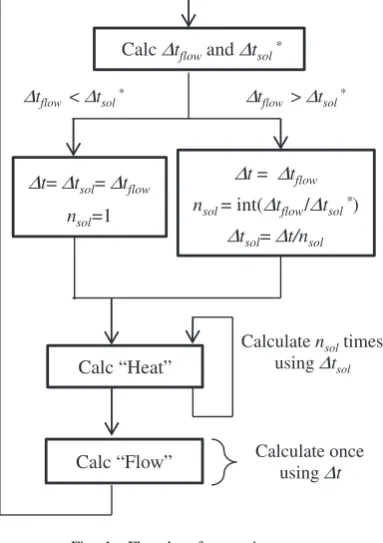
tflow, we performed the multiple heat transfer calculation in one time step in this study. A flowchart of calculation is shown in Fig. 1.tsol_{is the tentative value calculated using}

eq. (14), nsol is the number of iterations required for heat transfer calculation in one calculation cycle, and ‘‘int’’ is the operator used to generate an integer from a real number. First,

tflow and tsol are calculated. If tflow is smaller than

tsol, the common time increment t is determined to be equal totflow and all calculations are carried out once. In contrast, if tsol is smaller than tflow, then multiple heat transfer calculation is carried out. The number of iterations nsol is determined using tflow and tsol, so as to divide

tflow equally and to be minimum.

2.3 Application model

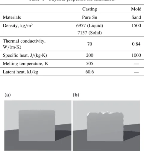
To evaluate the effectiveness and accuracy of the proposed MPS method, the solidification shrinkage problem was simulated using the method. The casting design and the initial arrangement of the melt and air particles are shown in Fig. 2 and Fig. 3, respectively. The initial specific size of the particles wasr0¼0:002m; thus, we used 3,465 particles

for the melt, 924 particles for air, and 35,096 particles for the mold in this study. Kinematic viscosity was set to 1:5107m2/s; the other parameters used in calculation are shown in Table 1. The heat resistance between different materials was assumed to be R¼0:0005m2_{K/W, so as to}

match the solidification time to the experimental result shown in section 3.2.1. The effect of solidification was taken into account by fixing the positions of the particles in space at a temperature below melting point.

CalcΔt_flowand Δt_sol*

Calc “Heat”

Calc “Flow”

Δtflow <Δtsol* Δtflow>Δtsol*

Δt=Δt_sol=Δt_flow n_sol=1

Δt= Δt_flow n_sol= int(Δt_flow/Δt_sol*₎

Δt_sol=Δt/n_sol

Calculate nsoltimes using Δtsol

Calculate once using Δt

Fig. 1 Flowchart for one time step.

35

(mm)

35

(a) Casting

74

64

(b) Mold

Casting

Fig. 2 Casting design.

(a) (b)

3. Calculation Stability

First, the flow and heat transfer simulations were combined and applied to a cylindrical pure Sn casting, and the stability of calculation was discussed in the case without air particles.

3.1 Numerical result

Figure 4 shows the calculated results of a still fluid without air particles (the arrangement of which is shown in Fig. 3(a)). The solidification effect (fixing the positions of the particles in space) was ignored. The cross section of the casting through the center was visualized using the free software POV-Ray 3.6. Figure 4(a) depicts the initial condition of the casting, and Fig. 4(b) shows the result 47 s after the simulation started. The velocity field diverged immediately after 47 s. Surface of the casting was uneven, because of the unusually high velocity of the particles. Approximately 5% of the particles went out of the cavity with a high velocity, and as a result, the surface level decreased, even though solidification and shrinkage were ignored. This unusually high velocity was produced because of a nonlinearity of the predictor-corrector method used in the MPS method, and the instability was caused by the calculation using the collocated calculation points of velocity and pressure. Tentative positions of the particles calculated in the prediction phase never moved back to the positions after the correction phase, and this caused the movement of the particles which led to an unnatural residual velocity. Therefore, we conclude that the MPS method is unsuitable for calculating the movement of particles in a still fluid and that sometimes the particles attain an unusually high velocity that causes divergence of the velocity field. In the case without air particles, the average velocity of the particles exceeded 0.02 m/s and the maximum velocity exceeded 0.2 m/s in the case of Fig. 4. In this case,

the particles during solidification are supposed to be almost still. Therefore, the calculated average velocity of 0.02 m/s is unacceptable. The problem of unusually high velocity could not be avoided using a smaller Courant number (i.e., a smaller time increment t), which indicates that it is impossible to correctly analyze the shrinkage behavior using the original MPS method.

3.2 Improvement of calculation stability

If the convection of the molten casting material can be assumed to be negligible during the shrinkage formation, the value 0.2 m/s of the maximum particle velocity as obtained in 3.1.1 is extremely unnatural. Let us suppose that the sur-face level descends by 0.01 m, solidification time is 100 s and the movement of the material is only caused by shrinkage; then, the maximum velocity of the particles at the descending surface of the casting would be about 0.0001 m/s. Thus, we propose a calculation method for the analysis of shrinkage formation under the following assumptions.

(1) Movement of the particles is only caused by shrinkage (density flow or convection induced by other-phenomena are ignored like creep flow).

(2) Given the assumption above, inertia force can be ignored. Viscosity is also ignored under the assumption that viscosity is not related to shrinkage formation in this study. Therefore, the tentative velocity and position in the pre-diction phase is caused only by gravity.

(3) Adjustment coefficient of gravity is introduced (eq. (15)) because natural gravity increases the tentative velocity to more than that required to describe the shrinkage formation.

gadjust¼g ð15Þ

Here,g(¼9:8m/s2_{) is gravity. Calculations were carried}

out using¼1, 0.1, and 0.01. If inertia force is ignored,umax is extremely small; therefore, time increment limitation by gravity is required. Assuming that the initial velocity is zero,

tshould satisfy the following equation.

tflow<Cn

ffiffiffiffiffiffiffiffiffiffiffiffiffiffiffi r0;ave jg_adjustj s

ð16Þ

The values of the maximum time increment were determined from test calculation to be as large as possible for stable calculation. The maximum time increment values used in this study were t¼0:001s (¼1), 0.002 s (¼0:1) and 0.01 s (¼0:01).

Figure 5 shows the results calculated by the original and proposed methods. In this case, solidification was considered. Figure 5(a) shows the result calculated by original method, using the value ¼0:01. Even with a weak gravitational force, the surface of the casting was uneven because of the unusually high particle velocity, which is similar to the case in which the solidification effect was ignored. Figure 5(b) shows the result calculated by the proposed method. In this case, cone-shaped solidification shrinkage was observed, as shown in Fig. 5(b). The original method resulted in an unusually high velocity, which in turn resulted in an uneven surface shape, while the proposed method calculated well-known cone-shaped shrinkage. In both methods, any change inshows almost no influence on the shrinkage shape.

Table 1 Physical properties for simulation.

Casting Mold

Materials Pure Sn Sand

Density, kg/m3 _{6957 (Liquid) 1500}

7157 (Solid)

Thermal conductivity,

W/(mK) 70 0.84

Specific heat, J/(kgK) 200 1000

Melting temperature, K 505 —

Latent heat, kJ/kg 60.6 —

(a) (b)

3.3 Discussion

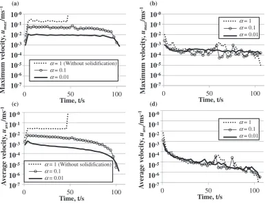
The series of results in the previous section show that the inertia force or viscosity caused unusually high velocity and an uneven surface shape. However, viscosity suppresses velocity growth, and therefore, an inertia force is expected to negatively affect the calculation of shrinkage formation. Figure 6 shows the maximum and average velocity variation with time. Figure 6(a) and (b) indicates the maximum velocity, while Fig. 6(c) and (d) indicates average velocity of particles. Figure 6(a) and (c) shows the results obtained by the original method (including the case of¼1without the effect of solidification), while Fig. 6(b) and (d) shows the results obtained by the proposed method. Figure 6(a) and (c) shows that a small value of reduced the velocity of particles; however, the values of the velocities remained at a high level. We can observe that the velocity of particles was greater than 0.01 m/s, even when ¼0:01. On the other hand, Fig. 6(b) and (d) shows that the velocity was extremely

low; almost all lines in the graphs were under 0.001 m/s. In addition, showed the little influence on the velocity. The results agreed well with the shrinkage shape calculated in section 3.1.2.

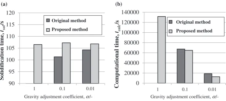
On the other hand, the use of a small value of (i.e. a larger t) reduces calculation time. Figure 7 shows the calculated solidification time and the calculation time. Calculation using original method diverged when ¼1 was used because the particles moved closer to each other owing to inertia and gravity. Because of this proximity, a strong repulsive force was generated between the particles, leading to the unusually high velocity of the particles and subsequent divergence of the calculation. In addition, as shown in Fig. 7(a), a large led to the calculated solid-ification time being shorter in the original method. A large value ofled to an increase in the particle velocity, which in turn increased the apparent thermal diffusivity. On the other hand, the results obtained by the proposed method showed a constant solidification time of approximately 107 s. Figure 7(b) indicates that calculation time could be reduced by using a smaller. The calculation time is almost inversely proportional to the maximum time increment. However, as in the case of the original method, t is limited by high velocity, according to eq. (13), and smaller t results in a longer calculation time.

Let us discuss the relationship between the amount of heat transfer and convection. Figure 8 shows the relationship between velocity and the Fourier number. The Fourier number Foindicates the relationship between heat transfer by convection and that by diffusion, as per the following equation.

(a) (b)

Fig. 5 Calculation results in the case of no air particles: cross section of casting after solidification. (a) Original method,¼0:01(b) Proposed method,¼1.

0 50 100

Time, t/s

0 50 100

Time, t/s

0 50 100

Time, t/s

0 50 100

Time, t/s

α= 1

α = 0.1

α = 0.01

10-1

10-5 10-4 10-3 10-2 10-0

10-6 10-7 10-1

10-5 10-4 10-3 10-2 10-0

10-6 10-7

Maximum v

elocity

,

umax

/ms

-1

α = 1 (Without solidification)

α = 0.1

α = 0.01

α = 1

α = 0.1

α = 0.01

A

v

erage v

elocity

,

uav

e

/ms

-1

10-1

10-5 10-4 10-3 10-2 10-0

10-6 10-7 10-1

10-5 10-4 10-3 10-2 10-0

10-6 10-7

A

v

erage v

elocity

,

uav

e

/ms

-1

Maximum v

elocity

,

umax

/ms

-1

α = 1 (Without solidification)

α = 0.1

α = 0.01

(a) (b)

(c) (d)

Fig. 6 Maximum and average velocity of particles. (a)umaxby original method (b)umaxby proposed method (c)uaveby original method

Fo¼ cp

1

lu ð17Þ

Here,l anduare specific length (m) and velocity (m/s), respectively. Parameters in Table 1 and l¼0:035m were used to calculate Fo. From Fig. 8, we find that Fois less than 1, if the velocity is greater than 0.001 m/s. Over this threshold, heat transfer is dominated by convection. This result agrees sufficiently with Fig. 6 and Fig. 7. Figure 6(a) and (c) shows that the velocity of the particles, as calculated by the original method, can exceed 0.001 m/s, and therefore, convection is the dominant heat transfer mechanism. In contrast, Fig. 6(b) and (d) shows that velocity of almost all particles, as calculated by the proposed method, is well below 0.001 m/s, and therefore, thermal diffusion is the dominant heat transfer mechanism. As a result, the original method led to an increased apparent thermal diffusivity and shorter solidification time which decreased with an increase of , while the proposed method showed a constant solidification time regardless of the value of.

Finally, we have to inquire the validity of the gravity adjustment coefficient. Ifis very small, the driving force for shrinkage formation becomes insufficient. Let us suppose that shrinkage formation is driven by gravity and only a descent of the surface level is considered, a requirement of

can be described as follows.

gttsol>lshrink ð18Þ

Here, t represents the time increment (s); tsol, solid-ification time (s); and lshrink, the depth of shrinkage (m). If tsol¼100s, lshrink ¼0:01m, and t is constant, the combinations oftandin section 3.1.2 satisfy eq. (18).

4. Influence of Air Cooling on Shrinkage Shape

In the next simulation, the influence of air cooling on shrinkage was examined using the proposed method. In this section, particle arrangement including air particles (as shown in Fig. 3(b)) is introduced. The parameters in Table 2 are used for the air particles. However, some assumptions about air particles, as detailed below, are made to ensure calculation stability.

(1) The density considered is greater than that of actual air in order to simplify the calculation. This is done because excessive difference between the densities of air and melt particles causes calculation instability; further, complex methods may be required if the actual density of air is used.1) (2) A larger than the normal value of thermal conductivity is used, because air convection is ignored.

(3) A smaller than the actual value of specific heat is used to compensate for the assumption of a larger value of density. Using these assumptions, calculations were carried out using different values of the specific heat of air particles, to investigate the influence of air cooling on the shrinkage shape.

4.1 Experimental result

Figure 9 shows an experimental result. The solidification time is approximately 80 s, and the heat transfer coefficient used in this study is adjusted on the basis of this time. We found that the external and internal shrinkages were

0 20000 40000 60000 80000 100000 120000 140000

calc

/s Original method

Proposed method

90 95 100 105 110 115 120

Solidif

ication time,

tsol

/s Original method

Proposed method

1 0.1 0.01 Gravity adjustment coefficient, α /-1 0.1 0.01

Gravity adjustment coefficient, α

/-Computational time,

t

(a) (b)

Fig. 7 Calculated solidification time and calculation time. (a) Calculated solidification time (b) Calculation time.

F

ourier number

,

Fo

/-Velocity, u/ms-1

0.0001 0.001 0.01 0.1 1 10 100 1000

0.00001 0.0001 0.001 0.01 0.1 1

Fig. 8 Relationship between velocity and Fourier number in pure Sn melt.

Table 2 Condition of air particles for simulation.

Density, kg/m3

Thermal conductivity,

W/(mK)

Specific heat, J/(kgK)

Case 1 5000 1 100

Case 2 5000 1 200

separated by a solidification shell. This separation was caused by air cooling; therefore, it is necessary to consider the influence of air cooling in reproducing the shrinkage formation behavior along with the separation.

4.2 Numerical results

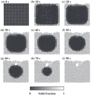
Figure 10 shows the calculation results under various air-cooling conditions. Figure 10(a) shows that no solidification shell was formed under weak air-cooling condition (Case 1). In contrast, in the case of stronger air-cooling condition (Cases 2 and 3), a solidification shell was formed and external and internal shrinkages were seperated (Fig. 10(b) and (c)). The solidification shell in Case 3 was thicker than that in Case 2 under stronger air cooling (Fig. 10(c)). Figure 11 shows the shrinkage formation behavior observed in Case 2 using a solid fraction. In Fig. 11, the cross section at the center of the casting is visualized using Micro AVS V.11. External shrinkage line

Internal shrinkage

Fig. 9 Experimental result.

(a) Case 1 (b) Case 2 (c) Case 3

Fig. 10 Influence of air cooling on shrinkage shape.

(a) 0 s (b) 10 s (c) 20 s

(d) 30 s (e) 40 s (f) 50 s

(g) 60 s (h) 70 s (i) 90 s

Solid fraction

0 1

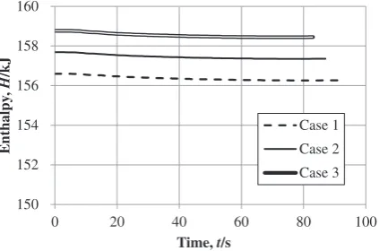
Figure 11 shows that the progression of shrinkage formation can be directly calculated; therefore, we infer that it can be considered more directly using the proposed method that the influence of the deformation of castings on other phenomena such as a variation of heat transfer paths or heat transfer conditions between materials. Finally, heat conservation was studied. The variation in the total enthalpy of the melt and the mold particles with time is shown in Fig. 12. The calculations in this study involved some discontinuity, such as the free surface and heat resistance between the melt and the mold. In addition, the Laplacian model for heat transfer calculation in eq. (4) was originally proposed for a continuum body consisting of particles with a uniform r0. In spite of these

limitations, Fig. 12 shows the heat conservation ability of the proposed method to be good. The enthalpy error during solidification was approximately 0.2%.

In this study, we proposed a simple coupling simulation program and applied it to shrinkage formation calculation. The results showed that the program based on the MPS method had high applicability to the casting problem. Although the calculations were carried out using a simple

shape and under many assumptions described in sec-tion 3.1.2, the MPS-based method has high applicability when incorporating many other effects such as temperature-dependent viscosity, surface tension, solute distribution, and thermal stress; therefore, further development of this method will enable calculation of more complex shapes and phenomena.

5. Conclusions

Heat transfer, solidification and flow simulation was combined based on the MPS method with temperature-dependent density, and direct simulation of shrinkage formation was carried out. First, the calculation stability for a still fluid was discussed. The instability encountered in the calculation was attributed to inertia force, and a method for improvement was proposed. The gravity adjustment coef-ficient was also introduced to reduce the calculation time. As a result, the calculation of the still fluid movement during solidification and the calculation of the influence of air-cooling on the shrinkage shape was carried out. Shrinkage formation behavior was also elucidated.

REFERENCES

1) S. Koshizuka:Ryushihou, (Maruzen, 2005).

2) S. Koshizuka:Ryushihou Simulation, (Baifukan, 2008).

3) S. Koshizuka, H. Tamako and Y. Oka: Comput. Fluid Dynamics J.4 (1995) 29–46.

4) S. Koshizuka and Y. Oka: Nucl. Sci. Eng.123(1996) 421–434. 5) S. Koshizuka, A. Nobe and Y. Oka: Int. J. Numer. Methods Fluids26

(1998) 751–769.

6) S. Koshizuka and Y. Oka: Nucl. Sci. Eng.123(1996) 421–434. 7) T. Belytchko, Y. Krongauz, D. Organ, M. Fleming and P. Krysl:

Comput. Methods Appl. Mech. Eng.139(1996) 3–47.

8) S. Shao and E. Y. M. Lo: Adv. Water Resour.26(2003) 787–800. 9) P. W. Cleary and J. Ha: Appl. Math. Model.30(2006) 1406–1427. 10) N. Hirata and K. Anzai: J. JFS80(2008) 81–87.

11) N. Hirata and K. Anzai: J. JFS83(2011) 259–267. 150

152 154 156 158 160

0 20 40 60 80 100

Enthalpy

,

H

/kJ

Time, t/s

Case 1

Case 2

Case 3