Agricultural competitiveness: The case of the European Union countries  

Competition is a component of the market economy and the feature of economic growth. It is defined as the rivalry in order to benefit from the economic activity. Due to the development of the international business environment and the increasing pressure of globalization, the importance of this phenomenon is also growing in all sectors of the economy, including agriculture (Kravčáková Vozárová 2013). Due to the broad meaning of competition, there is no agreement as to its measurement. According to the European Commission (2009), the most reliable indicator of competition in the long term is productivity.

The theory of trade suggests that a nation’s com-petitiveness is based on the concept of comparative advantages. In international comparisons, the com-petitiveness of agriculture is also assessed in the terms of cost. According to Latruffe (2010), the evaluation of competitiveness should be based on several ele-ments. However, the available studies usually include only one aspect of the evaluation. Regardless of the chosen measure, since competitiveness is a relative concept, this evaluation should be made in relation to the reference point. This justifies the comparison of countries or sectors with each other.

The purpose of this study is to identify the most im-portant factors of competitiveness of agriculture and

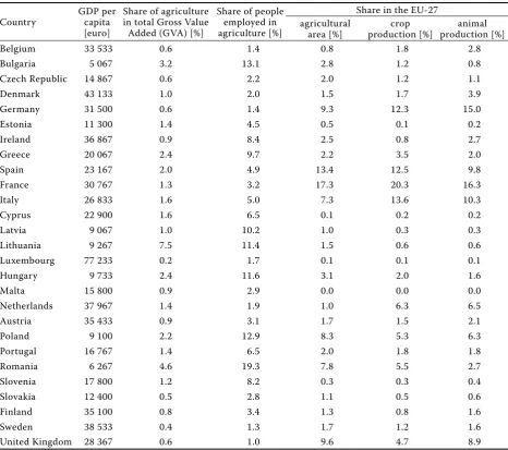
the evaluation of the European Union (EU) member states in terms of the competitiveness of the agricul-tural sector. It is important to take into account the specific conditions of the development of agriculture in the member states of the European Union. The results of research of many authors indicate consid-erable differences in the levels of development of the individual countries, including the level of develop-ment of agriculture (Arzeni et al. 2001; Serrão 2003; Fuller and Beghin 2007; Poczta and Fabisiak 2007). In the agricultural sector, these differences concern both its production potential and the effectiveness of its use. Table 1 presents the selected indicators characterizing agriculture of 27 EU countries, as well as a synthetic indicator of socio-economic develop-ment – GDP per capita.

As it can be seen from the data presented in Table 1, the highest level of development, measured by GDP per capita, is seen in such countries as Luxembourg (77 233 euro), Denmark (43 133 euro), Sweden (38 533 euro), the Netherlands (37 967 euro), Ireland (36 867 euro), Austria (35 433 euros), Finland (35 100 euros). However, in most countries that joined the EU in 2004 or later, the value of GDP per capita is significantly different from that reached by the so-called countries of the “Old 15”. The lowest level of development in the

Agricultural competitiveness: The case of the European

Union countries

Anna NOWAK, Agnieszka KAMINSKA

University of Life Science in Lublin, Lublin, Poland

Abstract: Th e paper assesses the competitiveness of agriculture of 27 countries of the European Union in the years 2009–

2011. Due to the complexity of the phenomenon of competitiveness, a wide range of variables was adopted to evaluate it – including the relationship between the production factors, productivity, and the importance of agriculture in the inter-national trade. Based on the evaluation criteria chosen for the competitiveness assessment and using the TOPSIS method, a synthetic measure of the studied phenomenon was constructed and then divided into four groups of countries similar in terms of the level of competitiveness of agriculture. Th e diff erence between the value of the synthetic measure of the coun-try with the highest level of competitiveness of agriculture (Netherlands) and the councoun-try least competitive in this regard (Slovenia) was 3.5-fold. In addition to the Netherlands, there were classifi ed also France, Germany, Denmark and Belgium in the fi rst group, so the countries with high levels of the socio-economic development. In the second group, there were se-ven countries: Italy, the United Kingdom, Spain, Cyprus, Austria, Ireland and Luxembourg. Th erefore, the fi rst two groups are formed by the countries belonging to the so-called “Old 15” (except Cyprus). Th e last two groups are formed primarily by the countries that joined the European Union in 2004 or later.

analysed period was visible in Bulgaria and Romania, where the analysed indicator accounted for 5067 Euro and 6267 Euro, respectively. As indicated by the Eurostat data, since the EU enlargement, the devel-opment gap which differs the individual countries, measured by GDP per capita, is reduced. This is also confirmed by the competitiveness ranking of the EU countries according to the HDI (Human Development Index), which measures the level of overall social and economic development. In the years 2004–2011, most “new” Member States improved their position in this ranking. The convergence process is, however, slow.

It can be also noted that in the countries with a lower level of development, agriculture is more important for the economy. Its share in the creation of Gross Value Added (GVA) reaches up to 7.5% in Lithuania.

This follows from the general regularities observed in many countries, according to which, along with an increase in the level of the socio-economic develop-ment of the country, there takes place a drop of the impact of agriculture on the macroeconomic indicators (Martino and Marchini 1996). This is also confirmed by the proportion of people employed in agriculture, which ranged from 1% in the United Kingdom to 19.3% in Romania, 13.1% in Bulgaria or 12.9% in Poland. The EU Member States have varying capabilities of agricultural production resulting from the existing resources of land. The greatest potential in this area have France and Spain, where the agricultural land makes a total of 30% of the EU-27 farmland. These countries are also the most important crop producers in the EU – in the years 2009–2011, they produced Table 1. Selected characteristics of agriculture in the EU countries (average for 2009–2011)

Country

GDP per capita [euro]

Share of agriculture in total Gross Value Added (GVA) [%]

Share of people employed in agriculture [%]

Share in the EU-27 agricultural

area [%]

crop production [%]

animal production [%] Belgium 33 533 0.6 1.4 0.8 1.8 2.8 Bulgaria 5 067 3.2 13.1 2.8 1.2 0.8 Czech Republic 14 867 0.6 2.2 2.0 1.2 1.1 Denmark 43 133 1.0 2.0 1.5 1.7 3.9 Germany 31 500 0.6 1.4 9.3 12.3 15.0 Estonia 11 300 1.4 4.5 0.5 0.1 0.2 Ireland 36 867 0.9 8.4 2.5 0.8 2.7

Greece 20 067 2.4 9.7 2.2 3.5 2.0

Spain 23 167 2.0 4.9 13.4 12.5 9.8 France 30 767 1.3 3.2 17.3 20.3 16.3 Italy 26 833 1.6 5.0 7.3 13.6 10.3

Cyprus 22 900 1.6 6.5 0.1 0.2 0.2

Latvia 9 067 1.0 10.2 1.0 0.3 0.3

Lithuania 9 267 7.5 11.4 1.5 0.6 0.6 Luxembourg 77 233 0.2 1.7 0.1 0.1 0.1 Hungary 9 733 2.4 11.6 3.1 2.0 1.6

Malta 15 800 0.9 2.9 0.0 0.0 0.0

Netherlands 37 967 1.4 1.9 1.0 6.3 6.5 Austria 35 433 0.9 3.1 1.7 1.5 2.1

Poland 9 100 2.2 12.9 8.3 5.3 6.3

Portugal 16 767 1.4 6.5 2.0 1.8 1.8 Romania 6 267 4.6 19.3 7.8 5.5 2.7 Slovenia 17 800 1.2 8.2 0.3 0.3 0.4 Slovakia 12 400 0.5 2.8 1.1 0.5 0.6 Finland 35 100 0.8 3.4 1.3 0.8 1.6

Sweden 38 533 0.4 1.3 1.7 1.2 1.6

more than 30% of its total value. These countries, along with Germany, also play the biggest role in the animal production – in the studied years, their par-ticipation in the EU production amounted to 41.3%. The smallest land resources used for agriculture and a small role in the agricultural production are noted on Malta, Cyprus, Luxembourg and Slovenia.

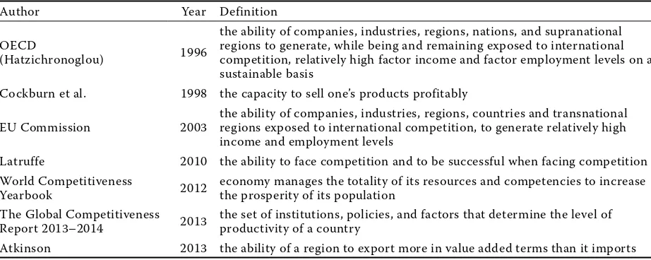
Considering this, the assessment of the competitive-ness of agriculture must be approached very carefully. The literature emphasizes that there is no single gen-eral theory relating to competitiveness; at different levels of analysis, a variety of different concepts is useful (Zawalińska 2004; Latruffe 2010). This is due to the fact that this concept has many dimensions, it applies to the individual behaviour, to the activi-ties of the company, sector, region, all the way to the national and transnational scale. Furthermore, the competitiveness can be defined as potential (estimated ex-ante) or actual (evaluated ex-post). Since the term was not consistently defined in the economic litera-ture, it has many different meanings. Each criterion of competitiveness also changes over time, accord-ing to the theory, and dependaccord-ing on the scale, which competitiveness concerns. Table 1 summarizes the most important, according to the authors, definitions of competitiveness.

Competitiveness is often only qualified without giving its definition. Porter, for example, does not define competition directly, but he refers the national competitiveness, to the level of regions, industrial and business clusters. In his concept of competitive advantage, he does not only take into account the supply and demand aspects of the research of

com-petitiveness, but also factors resulting from the theory of microeconomics and management at the level of the economic entities (Porter 2001). He indicates the determinants of national competitive advantage, which form the so-called “Porter’s Diamond”. These features include: (1) Firm Strategy, Structure & Rivalry; (2) Demand Conditions; (3) Related & Supporting Industries; (4) Factor Conditions (Porter 1990).

In the case of agriculture, the state intervention and agricultural policy also have a significant im-pact on competitiveness (Zawalińska 2004; Niezgoda 2009), and in relation to the EU member states – the Common Agricultural Policy. The importance of the state intervention in the agricultural market stems from the fact that the result of the permanent na-ture of investment in agriculna-ture, particularly land and part of the workforce, as well as the specifics of agricultural production, is the lack of possibility of an appropriate response by agricultural producers on changes in the market prices of agricultural products and the means of production (Grega 2002). This puts them at a disadvantage in the market. This applies especially to those countries where agriculture suf-fers from structural problems such as the agrarian fragmentation and overstaffing.

Many determinants shape productivity and com-petitiveness. Identification of these factors has been included in a number of theories, ranging from the Adam Smith’s theory based on the specialization and division of labour by the neoclassical economists with regard to the investment in the physical capital and infrastructure and, more recently, on the basis of other mechanisms, such as the education and

Table 2. Competitiveness definitions

Author Year Definition OECD

(Hatzichronoglou) 1996

the ability of companies, industries, regions, nations, and supranational regions to generate, while being and remaining exposed to international competition, relatively high factor income and factor employment levels on a sustainable basis

Cockburn et al. 1998 the capacity to sell one’s products profitably EU Commission 2003

the ability of companies, industries, regions, countries and transnational regions exposed to international competition, to generate relatively high income and employment levels

Latruffe 2010 the ability to face competition and to be successful when facing competition World Competitiveness

Yearbook 2012

economy manages the totality of its resources and competencies to increase the prosperity of its population

The Global Competitiveness Report 2013–2014 2013

the set of institutions, policies, and factors that determine the level of productivity of a country

training, technological progress, macroeconomic stability, good governance, and market efficiency (Schwab 2013). Cockburn et al. (1998) point out that a significant impact on the competitiveness of specific companies and industries in the market economy have the level of education, productivity, natural resources (neo-factorial theories), and the business-friendly economic policy. In agriculture, competitiveness is seriously determined by the input prices and by the subsidies (Korom and Sagi 2005).

The multitude of factors determining the com-petitiveness causes no agreement on the ways of the assessment of this phenomenon. In the studies, one can observe the trend of shifting from isolated indicators, often poorly capturing the spectrum of the determinants of competitiveness, to more com-plex approaches. Currently, among the concepts of modelling and measurement of competitiveness we can mark out indicators, rankings of competitiveness and models of competitiveness assessment (Józwiak 2012). Latruffe (2010), by reviewing the measures the competitiveness of agriculture, divides them into measures related to trade (trade measures of competi-tiveness) and measures of the strategic management (strategic management measures of competitive-ness), including, among others, the assessment of costs and productivity. Zawalińska (2004) emphasizes that there is no perfect measure of competitiveness. Nevertheless, most theories point to technology and productivity as the main determinants of the long-term competitiveness.

MATERIALS AND METHODS

Economic phenomena could be explained by using various methods. The commonly used approaches are the analytical description, the model approach and synthetic measures. The essence of synthetic meas-ures is the possibility of quantification by the use of a single factor of the phenomenon that is described in a large number of characteristics (Józwiak 2012). The difficulty of evaluating the competitiveness of agriculture is on the one hand due to the complex-ity and ambiguous nature of the phenomenon of competitiveness, and on the other hand, to the in-ternal diversity of agriculture and complexity of its surrounding.

The assessment of the competitiveness of agriculture was made for 27 countries of the European Union for the years 2009–2011. The analysis was based on

the standard results developed under the European system of the farm accountancy data collection – the Farm Accountancy Data Network (FADN), as well as the EUROSTAT data.

The variables describing the agricultural competi-tiveness:

Z₁ – land productivity (output per 1 ha of UAA lized agricultural area)

Z₂ – capital productivity (output per 1 Euro of the total fixed assets)

Z₃ – labour productivity (gross farm income per 1 Annual Work Unit)

Z₄ – total intermediate consumption per 1 ha of

UAA

Z₅ – gross investment per 1 ha of UAA

Z₆ – the value of the total fixed assets per 1 Annual Work Unit

Z₇ – the value of total fixed assets per 1 ha of UAA Z₈ – Farm Net Income per 1 hour of labour input Z₉ – the share of EU exports – food and live animals (%)

Z₁₀ – Trade Coverage Index [(food export/food im port))*100]

Z₁₁ – participation in the EU agricultural production (%)

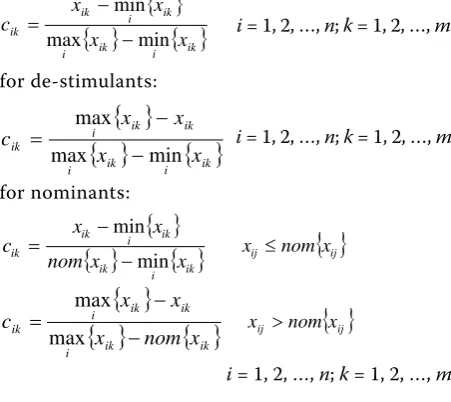
The analytical framework of the synthetic indicator comprises of three main stages, such as: the selec-tion of diagnostic features, the standardizaselec-tion of the chosen features and calculation of indicators value. In order to estimate the level of diversity of the en-vironment, a synthetic measure was used, based on VTOPSIS method (Technique for Order Performance by Similarity to an Ideal Solution) developed by Hwang and Yoon (1981).

X_[mxn] consisting of n alternatives and m attributes is constructed.

The procedure of the TOPSIS is summarized in five steps.

Step 1. Calculating the normalized evaluation matrix

The process is to transform different scales and units among various criteria into common measurable units to allow comparisons across the criteria. The normalized evaluation matrix C can be calculated by many normalization methods to achieve the objective. In order to normalize the features, the unitarization procedure was used based on the following formulas: for stimulants:

^ `

^ `

^ `

i ik i ik i ik ik x x x x c min max min

i = 1, 2, …, n; k = 1, 2, …, m

for de-stimulants:

^ `

^ `

^ `

i ik i ik ik i ik x x x x c min max max

i = 1, 2, …, n; k = 1, 2, …, m

for nominants:

^ `

^ `

^ `

i ik ik i ik ik x x nom x x c min min

xijdnom

^ `

^ `

^ `

^ `

i ik ik i ik x nom x x x c max max

xij !nom

^ `

i = 1, 2, …, n; k = 1, 2, …, m

Where:

 

max = maximum value of the k-th characteristic

 

min = minimum value of the k-th characteristic

Step 2. Determination of the positive ideal and negative ideal solution

The positive ideal solution A+ _{indicates the most}

preferable alternative and the negative ideal solution A– _{indicates the least preferable alternative.}

i c c c c c c

A max( 1),max( 2),...,max( ) 1, 2,...,

i c c c c c c

A min( 1),min( 2),...,min( ) 1, 2,...,

Step 3. Calculation of the separation measure The separation of each alternative from the positive ideal (d+) and negative ideal (d–) solution measures, using the n-dimensional Euclidean distance:

¦

i c c

d

1

2

i =1, …, n

¦

i c c

d

1

2

i =1, …, n

Step 4. Calculation of the relative closeness of each alternative to the ideal solution

The relative closeness of the i-th alternative with respect to the ideal solution A+ _{is defined as:}

     i i i i d d d

z , where 0z_i1

The larger the index value z_i, the better the perfor-mance of the alternative.

Step 5. Ranking the preference order

On the basis of the synthetic measure z_i, the mean and standard deviation administrative units were divided into four typological classes representing different level of the research issue:

– I class: zi zsz

– II class: zz_i zs_z – III class: zs_z z_i z – IV class: z_i zs_z

where: z– mean, sz– standard deviation.

RESULTS

Table 3 shows the statistical characteristics of diag-nostic variables adopted for the test.

In terms of values of the analysed variables, the in-dividual countries are characterized by a high degree of differentiation. The variation ranges from about 45% to 132%. The greatest diversity of the surveyed units is manifested in the case of variable Z11 – the participation in the EU agricultural production (%) and Z9 – the share of the EU exports – food and live animals (%). The smallest variation was seen in case of variable Z10 – the coverage of import by export expressed by the relation of food export to food import (%).

Both essential and statistic reasons decided about the diagnostic features selection. Moreover, the mu-tually strong correlated features were eliminated to dispose of the duplicate information. In order to elimi-nate the excessively correlated variables, an inverse matrix was established for the correlation coefficients between the assumed variables. On the basis of the analysis of the diagonal elements, the matrix Z₄ and Z₅ were eliminated from further investigations. All the analysed variables were considered stimulants.

competi-tiveness of agriculture was obtained. After the original matrix was created, the normalization of these values was calculated by using the formula in the fi rst step of the

TOPSIS method. Th e distances between the valuation subjects and the ideal and negative ideal solution were determined by taking the maximum and the minimum Table 3. Characteristics of the variables describing the competitiveness of the agricultural sector of the Member States of the European Union

Variable Mean Minimum Maximum Standard deviation

Coefficient of variation [%] Z₁ 2 579.7 589.02_{Latvia Netherlands}12 137.8 2 861.5 111.5 Z₂ 0.34 _Ireland0.06 _Slovakia0.98 0.21 61.4 Z₃ 28 696.4 _Romania5075.4 _Denmark91 092.4 21 406.3 75.2 Z₄ 1 695.9 _Lithuania443.1 8 778.2_Malta 1 937.2 114.3

Z₅ 442.44 _Romania63.13 _Netherlands21 12.5 483.9 109.1 Z₆ 245 638.8 _Romania19290.1 1 309 715.8_Denmark 285 646.4 116.5 Z₇ 11 697.4 _Slovakia855.02 61 736.6_Malta 14 523.2 124.2 Z₈ 4.98 _Slovakia–1.57 _France10.97 3.33 67.3 Z₉ 3.70 _Malta0.04 _Netherlands17.30 4.83 129.9

Z₁₀ 88.17 _Hungary23.91 _Cyprus160.31 39.44 45.1 Z₁₁ 3.70 _Malta0.03 _France19.16 4.91 132.2 Source: Own calculations based on data from the EU FADN and the EUROSTAT

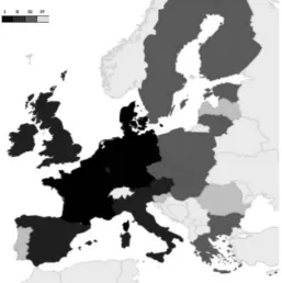
Figure 1.The classification of the Member States of the European Union in terms of the competi-tiveness of agriculture

values for each criterion from the normalization matrix table. Finally, the relative closeness calculation to the ideal solution was determined by using the formula in the fourth step of this method.

On the basis of the synthetic measure, obtained by the TOPSIS method, the countries were ranked and then divided into four typological groups with varying degrees of competitiveness of agriculture. The results of the analysis are presented in Table 4 and Figure 1. The mean values of variables for each typological group indexed according to the average obtained for Poland are presented in Figure 2.

DISCUSSION

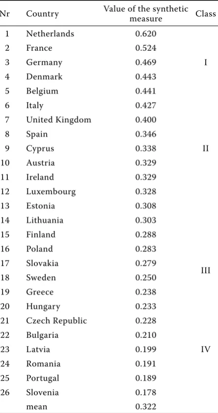
Synthetic measures describing the level of competi-tiveness of the agricultural sector adopted the values from 0.178 to 0.620, and for the majority of countries did not exceed the general mean value. The best rated was the Netherlands (the value of 0.620), and the worst Slovenia (the value of 0.178). In the first group, characterized by the highest level of competitiveness in agriculture, in addition to the Netherlands, there were classified also France, Germany, Denmark and Belgium. All these countries belong to the group of countries known as the “old 15”, they were members of the European Union before its biggest enlargement in 2004. Figure 2 shows the clear domination of these countries over other typological groups.

Except in rare cases, the values of the analysed diagnostic variables in these countries had good values in relation to the mean value calculated for all EU Member States. All mean values of the vari-ables in this group exceeded the general mean value. In particular, these countries were characterized by a very good productivity of land and labour, work equipment and technical infrastructure of land, as well as participation in the EU exports of food and live animals. It is worth noting that the countries belonging to the first group are characterized by high levels of the socio-economic development, as evidenced by the high level of the Gross Domestic Table 4. The classification of the Member States of

the European Union in terms of the competitiveness of agriculture

Nr Country Value of the synthetic _measure Class 1 Netherlands 0.620

I 2 France 0.524

3 Germany 0.469 4 Denmark 0.443 5 Belgium 0.441 6 Italy 0.427

II 7 United Kingdom 0.400

8 Spain 0.346 9 Cyprus 0.338 10 Austria 0.329 11 Ireland 0.329 12 Luxembourg 0.328 13 Estonia 0.308

III 14 Lithuania 0.303

15 Finland 0.288 16 Poland 0.283 17 Slovakia 0.279 18 Sweden 0.250 19 Greece 0.238 20 Hungary 0.233 21 Czech Republic 0.228 22 Bulgaria 0.210

23 Latvia 0.199 IV 24 Romania 0.191

25 Portugal 0.189 26 Slovenia 0.178 mean 0.322

Source: Own calculations based on data from the EU FADN and the EUROSTAT

0 0.5 1 1.5 2 2.5 3 3.5

Z1 Z2 Z3 Z6 Z7 Z8 Z9 Z10 Z11

I II III IV UE

Figure 2. The indexed values of variables in typologi-cal groups

Product (GDP) per capita. According to the Eurostat data, in 2012 the GDP per capita in the Netherlands, France, Germany, Denmark and Belgium accounted for, respectively, 144.1%, 120.4%, 126.8%, 169.4% and 132.4% of the mean value of this variable for 28 countries of the European Union.

In the second group, there were seven countries: Italy, the United Kingdom, Spain, Cyprus, Austria, Ireland and Luxembourg. Agriculture in those coun-tries was characterized by a high income per 1 hour of work (Z₈). Additionally, all of these countries except Cyprus and Luxembourg reported a high percentage of the participation in the EU agricultural produc-tion (Z₁₁) and an average Z9 – participation in the EU exports – food and live animals (%). The average values of the other diagnostic variables for this group fluctuated around the mean value for the EU, with the exception of the potential productivity of capital expressed by the value of agricultural production per 1 Euro of fixed assets (Z₂), which was low in all the countries belonging to this group.

The third group, with a low level of competitive-ness of agriculture, included ten countries (Estonia, Finland, Lithuania, Slovakia, Sweden, Poland, Hungary, Greece, the Czech Republic, Bulgaria). Seven of these countries are of a relatively low level of the socio-economic development – their accession to the EU took place in 2004 or in 2007. Finland is characterized by difficult natural conditions that are not conducive to the development of agriculture. The opportuni-ties of development for Greek agriculture are in turn limited by the mountainous character of the country and a little agricultural potential of the land. Capital productivity (Z₂) in this typological group was on a diverse level – in 6 countries it even exceeded the EU average. In this group, there were countries with different levels of the Trade Coverage Index (Z₁₀). Apart from a few cases, the values of other analysed diagnostic variables had negative values in relation to the mean value calculated for all EU Member States.

The fourth group, with the lowest level of com-petitiveness of the agricultural sector, included such countries as: Latvia, Romania, Portugal and Slovenia. Low competitiveness of agriculture in these countries should be connected, among others, with the low level of their development. The value of GDP per capita reached, respectively, 41.1%, 25.3%, 60.7% and 66.0% of the mean value for the 28 EU countries. Only the first three of these countries were characterized by the average capital productivity (output/total fixed assets) (Z₂), and Slovenia by a fairly good technical

infrastructure of the land (Z₇). In this group, the values of the other analysed variables had a low value.

The geographical presentation of the resulting division of the typological groups with respect to the selected analysed variables describing the level of competitiveness of the agricultural sector indi-cates the regional nature of the studied phenomenon (Figure 1).

CONCLUSIONS

The study assesses the competitiveness of agricul-ture of 27 European Union countries. A synthetic measure based on the TOPSIS method was used for this purpose. Then the countries were divided into four groups similar in terms of the level of competi-tiveness of the analysed sector. The added value of these studies and their contribution to the literature on the competitiveness of agriculture is confirmed by the used synthetic indicator, constructed on the basis of a broad set of variables characterizing the development of agriculture, its effectiveness, the relationship between the factors of production and the place in international trade.

Latruffe (2010), among others, draws attention to the advantages of such an approach to the research of the competitiveness of agriculture, which emphasizes the fact that the broad meaning of the concept of “competitiveness” determines the consideration of various components in its assessment. Using only indicators of productivity or only trade-related measures does not present a complete picture of the studied phenomenon. An additional advantage of the research is its scope, including the community of 27 countries of the European Union, which – ac-cording to the authors’ knowledge – is rarely carried out in relation to the assessment of the competitive-ness of agriculture.

countries, which manifests itself in, for example, a different soil quality, the length of the growing season, the structure of farms, or in the structure of agricultural production.

According to the adopted measure the countries with high levels of the socio-economic development (Netherlands, France, Germany, Denmark, Belgium) were among the countries with the highest levels of competitiveness. This means that there is a close relationship between the level of development of the national economy and the level of competitive-ness of agriculture. The results indicate, however, that the worst in the competitiveness ranking are primarily the countries whose accession to the EU took place in 2004 and later. It can be assumed that the competitive position of the individual countries in the coming years may vary as a result of the im-plementation of new principles of the Common Agricultural Policy. Among the instruments having a potential impact on improving the competitiveness of agriculture of the individual countries, especially those with a low level, we may mention more op-portunities of implementing innovations, some measures of promoting the transfer of knowledge, advisory services, the investment in physical assets and in the cooperation.

REFERENCES

Arzeni A., Esposti R., Sotte F. (2001): Agriculture in transi-tion countries and the European model of agriculture: entrepreneurship and multifunctionality. Report for the World Bank – Project “Šibenik-Knin and Zadar Coun-ties: Framework for a Regional Development Vision”, University of Ancona.

Atkinson R.D. (2013): Competitiveness, Innovation and Productivity: Clearing up the Confusion. The Informa-tion Technology & InnovaInforma-tion FoundaInforma-tion. Available at http://www2.itif.org/2013-competitiveness-innovation-productivity-clearing-up-confusion.pdf

Bulgurcu B. (2012): Application of TOPSIS technique for financial performance evaluation of technology firms in Istanbul stock exchange market. Precodia-Social and Behavioral Sciences, 62: 1033–1040.

Chen M.F., Tzeng G. H. (2004): Combining gray relations and TOPSIS concepts for selecting an expatriate host country. Mathematical and Computer Modelling, 40: 1473–1490.

Cockburn J., Siggel E., Coulibaly M., Vezina S. (1998): Measuring Competitiveness and its Sources: the Case of

Mali’s Manufacturing Sector. African Economic Policy Research Report, USAID, October.

Demireli E. (2010): TOPSIS multi-criteria decision-making method: an examination on state owned commercial banks in Turkey. Journal of Entrepreneurship and De-velopment, 5: 101–112.

EU Commission (2003): European Competitiveness Report 2003. Commission staff working document SEC(2003)1299. Available at http://aei.pitt.edu/45433/ (accessed Jan, 2015).

EU Commission (2009): European Competitiveness Report 2008. Brussels. Available at ec.europa.eu/enterprise/ newsroom/cf/_getdocument.cfm?doc_id (accessed Jan, 2015).

Fuller F., Beghin J.Ch. (ed.) (2007): European Agriculture: Enlargement, Structural Change, CAP Reform and Trade Liberalization. Nova Publishers, New York.

Grega L. (2002): Price stabilization as a factor of com-petitiveness of agriculture. Agricultural Economics – Czech, 48: 281–284.

Hatzichronoglou T. (1996): Globalisation and Competitive-ness: Relevant Indicators. OECD, STI Working papers 5. Available at http://www.oecd.org/officialdocuments/ publicdisplaydocumentpdf (accessed Feb, 2015). Hwang C.L., Yoon K. (1981): Multiple Attribute Decision

Making. Methods and Applications. Springer, Berlin. Janic M. (2003): Multicriteria evaluation of high-speed

rail, transrapid maglev and air passenger transport in Europe. Transportation Planning and Technology, 26: 491–512.

Józwiak W. (ed.) (2012): The Improve the Position of Polish Agriculture – Preliminary Proposals. IERiGŻ, Warszawa (in Polish).

Kaminska A. (2012): The application of the tools of spa-tial statistics to study regional differentation of polish environment. Colloquium Biometricum, 42: 111–119. Kołodziejczak A. (2010): Models of Spatial

Differentia-tion of Farming Methods in Polish Agriculture. UAM, Poznań.

Korom E., Sági J. (2005): Measures of competitiveness in agriculture. Journal of Central European Agriculture, 6: 375–380.

Kravčáková Vozárová I. (2013): The measurement of the competitiveness of EU agricultural production at the macroeconomic level. Exclusive Journal, Economy & Society & Environment, 1: 155–162.

Hatzichronoglou T. (1996): Globalisation and Competitive-ness: Relevant Indicators. OECD, STI Working papers 5. Available at http://www.oecd.org/officialdocuments/ publicdisplaydocumentpdf (accessed Feb, 2015). Martino G., Marchini A. (1996): The role of agriculture in

developed economies: new tendencies. MEDIT, 3: 26–30. Niezgoda D. (2009): Determinants of profitability of agri-cultural holdings diversified in respect of their economic size. Roczniki Nauk Rolniczych – Serie G, 96: 155–165 (in Polish).

Poczta W., Fabisiak A. (2007): Changes in labour force resources in agriculture in the Central and Eastern European Countries as a result of accession to the Eu-ropean Union. Roczniki Akademii Rolniczej w Poznaniu – CCCLXXXV, Ekonomia, 6: 109–117.

Porter M.E. (1990): Competitive Advantage of Nations. The Free Press, New York.

Porter M.E. (2001): Porter about the Competition. PWE, Warszawa (in Polish).

Schwab K. (ed.) (2013): The Global Competitiveness Report 2013–2014. World Economic Forum. Available at http://

www3.weforum.org/docs/WEF_GlobalCompetitiveness-Report_2013-14.pdf (accessed Feb, 2015).

Serrão A. (2003): Comparison of agricultural productivity among European countries. New Medit, 1: 14–20. Shih H.S., Shybur H.J., Lee E.S. (2007): An extension of

TOPSIS for group decision making. Mathematical and Computer Modelling, 45: 801–813.

Srdjevic B., Medeiros Y.D.P., Faria A.S. (2005): An objec-tive multi evaluation of water management scenarios. Water Resources Management, 18: 35–54.

World Competitiveness Yearbook (2012): IMD World Com-petitiveness Center. Available at http://www.imd.org/ wcc/wcy-world-competitivenessyearbook (accessed Feb, 2015).

Yang T., Chou P. (2005): Solving a multiresponse simulation – optimalization problem with discrete variables using multi-attribute decision-making method. Mathematics and Computers in Simulation, 68: 9–21.

Zawalińska K. (2004): The Competitiveness of Polish Agri-culture in the Context of Integration with the European Union. Warsaw University Department of Economics, Warsaw.

Received: 29th _{April 2015}

Accepted: 16th _{June 2015}

Published on-line 14th _{September 2016}

Contact address: