Functional morphology of proximal hindlimb muscles in the frog Rana pipiens

In recent years, neuromusculoskeletal modeling has become an important tool for understanding how muscles, tendons, joints and neural systems contribute to motor behaviors (Full and Ahn, 1995; Winters, 2000; Crago, 2000). Comparative animal models in particular have provided insight into motor control mechanisms that are common to most animals, e.g. spring-mass models of running (Cavagna et al., 1977), and into novel control solutions that are implemented by unique skeletomotor systems, e.g. dynamic turning in hexapods (Jindrich and Full, 1999). In the present study, we develop and describe the hindlimb musculotendon subsystem of a realistic model of the frog Rana pipiens. The frog represents an important experimental system for understanding the role of spinal circuits in movement construction (Giszter et al., 1993; Tresch et al., 1999; Kargo and Giszter, 2000a), musculotendon function during ballistic movements (Lutz and Rome, 1994, 1996a; Marsh, 1999), thermal effects on muscles and behavior (Rome and Kushmerick, 1983; Lutz and Rome, 1996b; Wilson et al., 2000) and the molecular basis of muscle contraction and motor performance (Gordon et al., 1966; Lutz and Lieber,

2000). Thus, a realistic model of the frog skeletomotor system might provide valuable insight into these important issues.

Before one can understand how the neural system controls limb behaviors or how molecular properties of muscle might affect performance, one must first have a clear picture of the mechanics of the limb. In particular, a substantial part of the control of any behavior is embedded in the anatomical and geometric design of the limb (Lombard and Abbot, 1907; Kubow and Full, 1999; Mussa-Ivaldi et al., 1985). Anatomical design features that affect the transformation of neural commands into force and movement may be classified as either macroscopic or microscopic features of the limb mechanical system (Lieber and Friden, 2000). Macroscopic features include those of the skeleton, e.g. bone lengths, joint degrees of freedom, moments of inertia and limb configuration, and those of the musculotendon complexes (MTCs), e.g. attachment sites, moment arms, muscle fiber lengths, in-series connective tissue lengths, cross-sectional areas and pennation angles. An important microscopic feature of the limb mechanical system is the internal sarcomere length of MTCs

JEB3958

Musculoskeletal models have become important tools in understanding motor control issues ranging from how muscles power movement to how sensory feedback supports movements. In the present study, we developed the initial musculotendon subsystem of a realistic model of the frog Rana pipiens. We measured the anatomical properties of 13 proximal muscles in the frog hindlimb and incorporated these measurements into a set of musculotendon actuators. We examined whether the interaction between this musculotendon subsystem and a previously developed skeleton/joint subsystem captured the passive behavior of the real frog’s musculoskeletal system. To do this, we compared the moment arms of musculotendon complexes measured experimentally with moment arms predicted by the model. We also compared sarcomere lengths measured experimentally at the starting and take-off positions of a jump with sarcomere lengths predicted by the model at these same limb positions. On the basis of the good fit of the experimental

data, we used the model to describe the multi-joint mechanical effects produced by contraction of each hindlimb muscle and to predict muscle trajectories during a range of limb behaviors (wiping, defensive kicking, swimming and jumping). Through these analyses, we show that all hindlimb muscles have multiple functions with respect to accelerating the limb in its three-dimensional workspace and that the balance of functions depends greatly on limb configuration. In addition, we show that muscles have multiple, task-specific functions with respect to the type of contraction performed. The results of this study provide important data regarding the multi-functional role of hindlimb muscles in the frog and form a foundation upon which additional model subsystems (e.g. neural) and more sophisticated muscle models can be appended.

Key words: muscle, hindlimb, musculoskeletal model, moment arm, force field, frog, Rana pipiens.

Summary

Introduction

Functional morphology of proximal hindlimb muscles in the frog Rana pipiens

William J. Kargo

_{* and Lawrence C. Rome}

1_{The Neurosciences Institute, 10640 John Jay Hopkins Drive, San Diego, CA 92121, USA and} 2_{Department of Biology, University of Pennsylvania, Philadelphia, PA 19129, USA}

*e-mail: kargo@nsi.edu

with respect to limb configuration (Burkholder and Lieber, 2001). The integration of these design features determines the movement ranges over which MTCs operate (Lieber and Friden, 2000), the moment-generating capabilities at particular limb positions (Murray et al., 2000) and the potential contributions of MTCs to endpoint force or limb stiffness (Buneo et al., 1997). Anatomically realistic models, which integrate experimentally measured properties of real animals, can be used to predict the operating ranges, moment-generating capabilities and endpoint force capabilities of MTCs and to estimate MTC trajectories during behaviors in which joint kinematics have been measured (Arnold et al., 2000; Delp et al., 1998; Hoy et al., 1990; Pandy, 2001).

In this study, we determined the anatomical properties of 13 proximal muscles in the frog hindlimb. We incorporated these properties into an accurate anatomical model of the frog. A previous study developed and described the skeleton and joint subsystems of this model (Kargo et al., 2002). We validated the interaction between the hindlimb musculotendon and joint subsystems by comparing moment arms measured across the configuration-space of the hindlimb and sarcomere lengths measured at the starting and take-off positions of a jump with moment arms and sarcomere lengths predicted by the model at these same limb positions. We then used the model to describe the static, whole-limb effects of each of the hindlimb muscles as a three-dimensional force field. The force-field measurements summarize how a muscle contraction will act to accelerate the limb from a large range of limb configurations (Giszter et al., 1993; Loeb et al., 2000). We also use the model to predict MTC trajectories during a number of hindlimb behaviors (wiping, kicking, swimming and jumping) and to estimate the contractile function of specific MTCs during these behaviors. The results of this study provide a useful summary of the static mechanics of the pelvic/hindlimb system of the frog. More importantly, the model forms a foundation upon which additional subsystems (e.g. neural systems) and more sophisticated muscle models can be appended to examine the dynamic control of limb behaviors.

Materials and methods Musculotendon attachment sites

The origin and insertion sites of 13 proximal muscles in the hindlimb of Rana pipiens were determined. Frogs were killed with an overdose of Tricaine (Sigma Aldrich) and pithing in accordance with IACUC protocol. The hindlimb/pelvis complex was removed, and individual muscles were partially dissected and allowed to dry out at right angles to the bone segments. The pelvis and hindlimb segments (femur, tibiofibula, astragalus–calcaneus and metatarsal–phalangeal segments) were disarticulated from one another and laser-scanned using a three-dimensional laser scanner (Cyberware Inc., Monterey, CA, USA) controlled by a Silicon Graphics O2

Unix computer. The laser scanner has a resolution of 50µm. The individual bone segment with its muscle attachments intact was placed on a rotating stage, and one surface scan was

taken. The stage was rotated 36 times by 10 ° (by 360 ° in total) to obtain a complete three-dimensional scan. The bone/muscle complex was reoriented on the stage, and a second complete scan was taken. Five complete scans were taken and merged to produce a single three-dimensional image file (see Fig. 1).

The image file was imported into SIMM (Software for Interactive Musculoskeletal Modeling, Musculographics Inc., Santa Rosa, CA, USA), which is a graphics-based, biomechanical modeling package. A second laser-scanned image of the bone, one in which the muscles had been completely removed, was also imported into SIMM and overlaid on the first image. The attachments of virtual muscles in SIMM were manually positioned on this second bone segment. The hindlimb muscles whose attachment sites were determined were the semimembranosus (SM), gracilus major (GR), adductor magnus dorsal and ventral heads (ADd and ADv), cruralis (CR), gluteus magnus (GL), semitendinosus ventral and dorsal heads (STv and STd), iliofibularis (ILf), iliacus externus (ILe), iliacus internus (ILi), sartorius (SA) and tensor fascia latae (TFL).

In the model, the paths for 10 of the hindlimb muscles were represented as a simple straight line from an origin point to an insertion point (all muscles but STd, STv and ILe). The paths for STd and STv between the origin and insertion points were constrained by an intermediate via-point added 2.0 mm posterior to the knee joint. This via-point approximates the effect of a connective-tissue loop, which constrains ST paths in real frogs (Lombard and Abbot, 1907). The path for ILe between its origin and insertion points was constrained by an intermediate via-point positioned just ventral to the GL attachment on the pelvis. The path for the triceps muscle group (CR, GL and TFL) was constrained to wrap over the anterior knee joint. The shape of the wrap object that deflected the triceps muscles approximated the distal surface of the femur. A second wrap object, which approximated the geometry of the femoral head, prevented muscles from penetrating the femoral head in the extreme ranges of hip rotation. A third wrap object approximated the posterior surface of the distal femur and deflected knee flexor muscles (ST, GR, ILf and SA) in the extreme ranges of knee extension.

Moment arm measurements

muscles about the three axes of the hip joint and about the primary axis of knee rotation. We then tested whether the model moment arms matched the moment arm measurements made in experimental frogs.

The method used to measure moment arms experimentally was the ‘tendon excursion method’. This method has been used previously in our laboratory and described in detail (see Lutz and Rome, 1996b). Briefly, all muscles were removed from the hindlimb except the muscle under study and small muscles surrounding the joints. One bone segment (e.g. the pelvis) was secured into the fixed arm of a custom-built jig apparatus, and its distal joint member (e.g. the femur/tibiofibula complex) was secured into the movable arm of the jig. The movable arm permitted 180 ° of rotation and unopposed translation of the distal segment within two orthogonal planes of motion. The muscle attachment on the fixed segment was detached. A thread was tied to the detached tendon of the muscle and run over a length scale and pulley. A 20 g weight was suspended from the end of the thread to maintain a constant tension. The change in the length of the muscle was measured as the moving arm of the jig was rotated. The moment arm (r) about an axis of rotation was calculated using the following equation:

r = ∆L/∆θ, (1)

where θ is the joint angle; ∆θ was 0.1745 rad (or 10 °), and muscle length (L) was measured on the length scale.

We used a modified technique, similar to that used by Delp et al. (1999), to measure the moment arms of smaller muscles and muscles with little tendon in which to tie the thread around (ADd, ADv, ILe, ILi, ILf, STv, STd, SA). A miniature bone screw was placed at the insertion site of the muscle in the moving segment. A suture thread was tied around the screw. A minutien pin (i.e. an insect pin) with a loop at one end was placed at the muscle origin on the fixed segment. The suture was threaded through the loop and run over the length scale, and a 5 g weight was suspended from the end of the thread. The change in the length of the suture thread was measured as the moving arm of the jig was rotated. The moment arm was calculated using equation 1.

The moment arms of muscles crossing the hip joint were measured with respect to an xyz coordinate system embedded in the femur (see Fig. 3). When all the bones rested in the horizontal plane, the z-axis of the femur pointed dorsally. For the right hip, clockwise rotation of the femur about the z-axis was extension and counterclockwise rotation was flexion. The x-axis of the femur pointed down its long axis. When looking up the x-axis (proximal to distal), clockwise rotation of the femur was external rotation and counterclockwise rotation was internal rotation. The y-axis of the femur pointed rostrally when the femur was positioned to the frog’s side and in the horizontal plane. When looking up the y-axis (rostral to caudal), clockwise rotation of the femur was abduction and counterclockwise rotation was adduction.

The moment arms of muscles crossing the knee were measured only with respect to the z-axis of the knee joint (see Fig. 3). The z-axis pointed dorsally when the hindlimb was

positioned in the horizontal plane and was located along the distal surface of the femur. The z-axis was translated along the distal surface of the femur with tibiofibula rotation (see Kargo et al., 2002). For the right knee, clockwise rotation of the tibiofibula about the z-axis was flexion and counterclockwise rotation was extension.

In total, 27 frogs were used to measure moment arms at the hip and knee joints. Moment arm measurements performed in individual frogs were normalized to combine data among frogs. To normalize the data, we assumed that all frogs were geometrically similar. In our study, an averaged-sized Rana pipiens weighed 28±4 g (mean ± S.E.M.) and had a tibiofibula length of 30±3 mm (mean ±S.E.M.). Also, all frogs (three frogs) whose bones were laser-scanned to construct the hindlimb model weighed 28 g and had a tibiofibula length of 30 mm. Thus, moment arm measurements were normalized to a tibiofibula length of 30 mm. For example, a moment arm measurement of 3.0 mm made in a frog with a tibiofibula length of 32 mm was normalized to 2.8 mm, i.e. 3.0×30.0/32.0.

The moment arm about a single axis of hip rotation can vary as the angle about the other two axes of the hip is changed (Arnold and Delp, 2001). Since the jig allowed simultaneous and independent rotations about two joint axes, we examined the nature of such interactions for hindlimb muscles in the frog.

θ1(e.g. hip abduction angle) was fixed at a specific value, and

θ2(e.g. hip extension angle) was changed in 10 ° increments.

The moment arm with respect to θ2was determined. θ1was

then rotated to a new angle, and the same series of θ2rotations

was imposed. The data for such an experiment were evaluated using three-dimensional plots (Matlab, Mathworks Inc., Natick, MA, USA). The horizontal axes in the plots represented the angles θ1 and θ2, and the vertical axis

represented the moment arm with respect to θ2. Joint angle

interactions were tested for in four representative muscles that cross the hip joint: SM (five frogs), GR (four frogs), SA (five frogs) and GL (three frogs).

Musculotendon architecture

We measured physiological cross-sectional area (PCSA), sarcomere length/joint angle relationships, muscle fiber lengths and in-series connective tissue lengths for each of the proximal hindlimb muscles. These parameters have previously been measured for some muscles in Rana pipiens. Calow and Alexander (1973) and Lieber and Brown (1992) published values for CR, Plantarus ankle extensor (PL), GL, SM, GR, STv and ILi. We determined these parameters for six additional muscles in Rana pipiens and for the same seven muscles for comparison purposes.

PCSA was determined using the following relationship:

where ρis muscle density (1.056 g cm–3_), α_{is pennation angle,} mmis muscle mass and lOMis the optimal muscle fiber length

for force generation. Muscle mass was measured directly.

(2) PCSA = mmcosα ,

Pennation angle (α) was estimated using caliper measurements from dissected muscles. lOM was measured as the muscle

fascicle length at which sarcomere length was optimal for force generation (2.2µm in the frog; Gordon et al., 1966). Measurement of lOMis described below.

Sarcomere lengths were measured in both fixed and frozen muscle tissue at a single test position. The test position was a planar configuration in which the femur was extended by 90 ° relative to the long axis of the pelvis and the tibiofibula was extended by 90 ° relative to the femur (see Fig. 2). The pelvis/limb complex was secured in the test position using bone pins, fine steel wire and hardening epoxy resin. For fixed tissue measurements, the complex was sequentially immersed in 0.05 % formalin solution for 8 h, 10 % formalin solution for 24 h and 30 % nitric acid for 4 h, and then washed in distilled water. Small fascicles were dissected from each hindlimb muscle, and their lengths were measured with a stage graticule. In-series connective tissue length was found by subtracting fascicle length from whole-muscle length. The fascicle was placed on a slide and mounted in glycerine. Sarcomere lengths were measured at three regions along the length of the fascicle by counting 30 sarcomeres in series, measuring the length from the first to the last sarcomere under a calibrated eyepiece graticule and dividing by 30. Care was taken to dissect fascicles from similar anatomical regions of each muscle in all the frogs. For example, in thinner strap-like muscles such as SA, fascicles were dissected from a middle region and from regions bordering adjacent muscles. For thicker, architecturally more complex, muscles such as CR, fascicles were dissected from superficial, middle and deep regions of the muscle belly.

For sarcomere length measurements in frozen tissue, the limb was secured in the test position and glycerinated in cold rigor solution (15 ml potassium phosphate buffer, 100 mmol l–1 _{potassium acetate, 5 mmol l}–1 _K

2EGTA,

1 mmol l–1 _{iodoacetic acid, 0.1 mmol l}–1 _leupeptin,

0.25 mmol l–1 _{phenylmethylsulfonyl fluoride and}

0.01 mmol l–1 _{pepstatin, pH 7.2) for approximately 2 days.}

Sosnicki et al. (1991) determined that this method allowed fibers to go into complete rigor. The limb complex was then quickly and entirely immersed in liquid-nitrogen-cooled isopentane. Frozen blocks were cryo-sectioned along the long axis of the muscle in sections 25µm thick and examined under the light microscope. Both techniques (fixation and freezing) were used because of trade-offs between the two. Frozen tissue measurements have been shown under certain circumstances to be more accurate for determining in vivo sarcomere lengths (Sosnicki et al., 1991). However, the fixed tissue procedure allowed sarcomere lengths to be measured simultaneously in more muscles, i.e. in frozen blocks, it is difficult to distinguish muscles so only one or two muscles were left intact. Thus, the freezing technique was used mainly to validate measurements made in fixed tissue. We found that sarcomere lengths were, on average, 5–7 % shorter in fixed tissue than in frozen tissue. Thus, a correction factor (0.05) was applied to all fixed tissue measurements, e.g. a sarcomere

length of 2.00µm in fixed tissue was multiplied by 0.05 (+2.00µm) to produce a corrected sarcomere length of 2.10µm.

Validating model predictions of sarcomere length We measured sarcomere, fascicle and whole-muscle lengths of each muscle at the test position in six frogs. We then positioned the model hindlimb at the same test position. Because we measured the lengths of sarcomeres and muscle fibers undergoing fixed-end contractions (i.e. when in the rigor state), we could not simply assign each ‘non-contracting’ muscle in the model the experimental measurements. Sarcomeres are arranged in series with connective tissue that is stretched during muscle contraction and may therefore shorten by up to 20 % during fixed-end contractions (Lieber et al., 1991; James et al., 1995). To assign the model muscles the correct, non-contracting values for in-series connective tissue, muscle fiber and sarcomere length, we had to estimate the non-contracting lengths. This was performed as detailed below.

First, we assumed that in-series connective tissue (for each muscle) exhibited an ideal stress/strain relationship, which is similar to that described for the frog plantarus tendon (Trestik and Lieber, 1993), and a strain at maximal tetanic tension equal to 3.5 %. We chose 3.5 % as a general measure for each muscle because the in-series connective tissue of frog muscles exhibits strains that range, on average, from 2 to 5 % (Lieber et al., 1991; Trestik and Lieber, 1993; Kawakami and Lieber, 2000). Second, we determined the ratio of connective tissue length to muscle fiber length for each muscle at the test position (see Table 1). Third, we assumed that frog sarcomeres exhibit an ideal sarcomere length/tension relationship, which has been described by Gordon et al. (1966). On the basis of these three relationships and the measured sarcomere length at the test position, we estimated the non-contracting sarcomere length. For example, muscle A had a measured sarcomere length of 2.2µm. Frog sarcomeres produce their maximal tetanic force at this length (Gordon et al., 1966). This level of force stretches the in-series connective tissue by 3.5 %. Thus, if the measured lengths of in-series connective tissue, muscle fiber and sarcomere were 10.35 mm, 10.00 mm and 2.20µm, respectively, the non-contracting lengths would be 10.00 mm, 10.35 mm and 2.28µm, respectively. However, the 13 proximal muscles of the frog hindlimb have a mean connective tissue/muscle fiber ratio of only 1.04. Thus, the sarcomere shortening effect was not substantial (i.e. these muscles are ‘stiff’ actuators). This effect only becomes substantial when ratios approach 5.0–10.0 (Zajac, 1989; Lieber et al., 1991; James et al., 1995).

sarcomere lengths on the basis of moment arm variations across the configuration-space of the limb:

FL = FLP+ ∆FL , (4)

where FL is fascicle length, r represents the moment arm of the musculotendon complex (MTC), MTCPand FLPrepresent

the MTC and fascicle lengths measured at the test position, α is pennation angle and ∆θ (the change in joint angle) is in radians. Sarcomere length (SL) was calculated in the same way by substituting SLP for FLP in equations 3 and 4.

Pennation angle was assumed to be constant at all positions, which is a reasonable assumption for muscles with pennation angles of less than 20 ° (see Zajac, 1989; Cheng et al., 2000). Thus, we expected that only our predictions for CR (α=20–25 °) might be significantly affected by this assumption (see Table 2 for values of αfor muscles). If our model predictions for CR were very different from experimental measurements, then alternative models (e.g. finite-element models), which account for configuration-dependent changes in pennation angle, will ultimately have to be developed and used.

To test the model predictions, we compared sarcomere lengths measured in experimental frogs at the starting and take-off positions of a jump with sarcomere lengths calculated at these same positions in the model. The three-dimensional kinematics of jumping was previously determined and used to position both experimental frogs and the model (Kargo et al., 2002). To measure sarcomere lengths experimentally, the right limb was fixed at the starting configuration of a jump by wrapping fine steel wire around bone screws placed in the hindlimb segments. A hardening epoxy compound secured the wires in place. This start position was 30 ° hip flexion, 15 ° internal rotation, 18 ° hip adduction and 65 ° knee flexion. Angles were determined in the jig apparatus. The left limb was then fixed at the approximate take-off position. This position was –75 ° hip extension, 0 ° internal rotation, 0 ° hip adduction and –75 ° knee extension. The muscle/limb complex was then fixed, the fascicles were dissected and the sarcomere lengths were measured using the procedure described above. The correction factor (0.05) was applied to account for the additional shortening due to the fixative.

We used the following procedure to predict the length of ‘contracting’ sarcomeres in the model at the start and take-off positions of a jump. We simulated fixed-end contractions for each musculotendon actuator at the two limb positions. Each actuator produced a contractile force that was derived from scaling generic musculotendon properties with five muscle-specific parameters. The muscle-muscle-specific parameters were: PO,

peak tetanic force; lOM, optimal muscle fiber length, α,

pennation angle; lOT, length of in-series connective tissue; and

εOT, strain of in-series connective tissue when force in the

tendon PT_=P

O. PO was estimated for each muscle by

multiplying PCSA by muscle stress, which Lutz and Rome (1996b) measured in the SM muscle to be 260 kN m–2_{. The SM}

muscle is composed of 85–90 % fast muscle fibers, and the other hindlimb muscles have similar high percentages of fast muscle fibers (Lutz et al., 1998). Thus, assuming that all hindlimb muscles had a muscle stress equal to 260 kN m–2_is

reasonable. Although this assumption will affect the contractile force that each model actuator is capable of producing, it will not affect the calculation of sarcomere or muscle fiber lengths in the model. The reason for this is that tendon properties were assumed to be matched to muscle properties, i.e. tendon strain (at PO) was 3.5 % irrespective of how much force each actuator

produced.

In contrast to PO, we measured αdirectly at the test position,

and lOMand lOTwere the muscle fiber and in-series connective

tissue lengths at the limb position in which sarcomere length was 2.2µm. The generic musculotendon properties that were necessary for calculating muscle fiber lengths during the fixed-end contraction were: the ideal muscle sarcomere length/tension relationship described by Gordon et al. (1966), the ideal muscle fiber velocity/force relationship (vCE_/PCE₎

described for the frog sartorius muscle by Edman et al. (1979) and the exponential stress/strain (PT_/εT_{) relationship of the}

tendon described by Trestik and Lieber (1993) where PT_{is the}

force in the tendon in-series connective tissue. Thus, the contractile force in response to maximal activation [a(t)=1.0] of a model actuator could be described by the following:

PCE_{= [P}CE_lM_{· a(t)] · P}CE_(vCE_{) , (5)}

where fiber velocity (vCE_{) was found by solving equation 5 for} vCE_. α_{was assumed to be constant in the fixed-end contractions}

and thus to result in the following:

PT_{= P}M_cosα_{, (6)}

lMT_{= l}T_{+ l}M_cosα_{, (7)}

and

vMT_{= v}T_{+ (v}CE_/cosα_{) , (8)}

where PM_{is the force in muscle fibres, v}MT_{is the velocity of}

musculotendon complex, lMT_{is musculotendon length, l}T_is

in-series connective tissue length and lM_{is muscle fiber length.}

The final equation used for describing the dynamics of the simulated fixed-end contractions was:

where t is time and f defines a function. Muscle activation dynamics was simulated in Matlab Simulink (using a first-order dynamic equation; see equation 10; activation time constant c1=13 ms, deactivation time constant c2=50 ms). To

avoid inaccuracies in representing the dynamics of the activation transients, we calculated force and sarcomere lengths only at 500 ms after the onset of the simulated contraction. The time step used in the dynamic simulations was

(9) = f [PT_,lMT_,vMT_{,a(t)] ,}

dPT

dt (3)

∆FL = · FLP· cosα ·∆θ r

MTCP

  

5 ms, and the equation describing the first-order activation dynamics was represented as:

where u represents the excitation signal used to activate the muscle (i.e. a step signal of 1 s), aM_{represents the activation}

level of the muscle and a˙M_{is the first derivative of a}M_where c1is 1/activation time constant (15 ms) and c2is 1/deactivation

time constant (50 ms). Sarcomere lengths calculated at the start and take-off positions in the model were compared with sarcomere lengths measured experimentally.

Determination of static muscle functions

We used the hindlimb model to describe the static mechanical effects of each muscle. The state space of muscle effects was described as an isometric force field (see Giszter et al., 1993; Loeb et al., 2000). To construct a force field, the ankle of the model limb was placed at 80 different positions throughout the hindlimb’s reachable workspace. The reachable workspace refers to the three-dimensional area over which the ankle can be positioned. The workspace was divided into five levels. The top level was 15 mm above the horizontal plane of the pelvis (z=+15 mm), the bottom level was 15 mm below the plane of the pelvis (z=–15 mm) and the middle level was at the plane of the pelvis (z=0 mm). The other two planes were +7.5 mm above and –7.5 mm below the plane of the pelvis. The ankle was placed at 16 different positions (x1–16,y1–16) within

each horizontal level. These x,y positions were the same for each level. The 80 positions spanned the reachable workspace of the limb and formed a three-dimensional box.

To construct muscle force fields, we simulated fixed-end contractions of each musculotendon actuator at each position. The actuators were maximally activated, and the contractile force was calculated 500 ms into the simulation run. At each position, the contractile force of the muscle produced a set of joint moments about the hip and knee. Joint moments were calculated automatically in SIMM by multiplying muscle force by the respective moment arm. The joint moments were then transmitted through the hindlimb to produce a force at the ankle. This force (F) was calculated using the following relationship (Tsai, 1999):

F = (JT₎–1τ_{, (11)}

where JT_{is the transpose of the Jacobian matrix describing the}

configuration and segment lengths of the hindlimb (Tsai, 1999; Kargo et al., 2002), and τis the matrix of joint moments at the current position and resulting from muscle contraction. The force measured at the ankle represents the force that the ankle exerts against an immovable obstacle, e.g. a force sensor, and has three vector components. The z component of the force vector was the vertical force that the ankle exerts on an object impeding its movement. The x and y components were the mediolateral and rostrocaudal forces, respectively, within the (five) horizontal levels of the sampled workspace. Muscle

force fields were graphically presented as three-dimensional and two-dimensional plots.

Results

Attachment sites and paths of proximal hindlimb muscles The hip joint complex from four separate frogs was laser-scanned. The SM, GR, ADd and ADv tendons were left intact on the pelvis of one complex. The GL, ILf, CR and SA tendons were left intact on a second pelvis. The STv, STd, ILe and ILi tendons were left intact on a third pelvis. All tendons except for SM and CR were left intact on a fourth pelvis. This fourth pelvis is shown in Fig. 1A, and the locations in which the muscles attached to the pelvis are marked. These locations were determined from the previous scans in which only a few (four) muscles had been left intact and where it was easier to differentiate the individual attachment sites. The attachment sites were superimposed on the fourth scan. The attachment sites for STd and STv are not shown in Fig. 1A because they are embedded under the larger GR and ADd muscles (only the more distal portions of the tendons are shown). The attachment sites of additional muscles whose architectural and anatomical properties are not presented in this study are also shown in Fig. 1A. These muscles are the obturator internus (OI), the quadratus femoris (QF) and the pectineus (Pec).

The knee-joint complex from three separate frogs was laser-scanned. The ST, ILf and CR, GL and TFL (triceps group) tendons were left intact on the tibiofibula in one knee complex. The GR, SA and SM tendons were left intact on a second complex. GR and SA attached to the tibiofibula and SM attached to the posterior surface of the distal femur and knee capsule. All the tendons were left intact on a third knee complex. This third complex is shown in Fig. 1B. The attachment sites of additional distal muscles (actions at the ankle and tarso-metatarsal joint) are also shown in Fig. 1B. These muscles are the plantarus (PL), tibialis anterior (TA) and peroneus (PE) muscles.

The modeled paths of the proximal hindlimb muscles are shown in Fig. 2. The top four panels show the paths of hip-flexor muscles (CR, GL, ILe, ILf, ILi, Pec, SA and TFL). The bottom four panels show the paths of hip-extensor muscles (ADd, ADv, GR, OI, OE, QF, SM, STd, STv). Some muscle paths were constrained to wrap around certain skeletal features. The distal path of the triceps group (CR, GL and TFL) wrapped over the knee joint. The distal path of ILe wrapped over the femoral head. In the extreme ranges of hip flexion and hip extension, both extensor and flexor paths were constrained to wrap around the femur. In addition, in the extreme range of knee extension, the ST, ILf, GR and SA tendons were constrained to wrap around the posterior surface of the distal femur.

Moment arms about the hip joint

We measured the moment arms about the flexion–extension axis of the femur (z-axis) in experimental frogs (see z-axis in Fig. 3). The limb configuration in Fig. 3 was the test position

  

 

, (10)

a˙M₌ (u−aM) · (c1u + c1) ,

(u−aM_{) · c} 2

Femur

Tibiofibula SA

GR

ST

SM PL GR

SA ILf

ST

ILf

PL CR GL TFL

SA

GR TA–PE

ILf PE,TA SM

STd

STv

STv ILe

ILi

ILe

ILi CR GL ILf SM

GR

ADd,v OI

SA Pec

TFL ADv

Pec SA

ILf

GL

ADd

GL ILf

ILi

SA GR

SM

QF

ADv

Pelvis–femur complex

A

B

Fig. 1. Muscle attachment sites in the frog Rana pipiens. (A) Attachment sites on the pelvis. The thigh muscles were dissected, and the proximal portion of each muscle, except CR (cruralis) and SM (semimembranosus) in this particular specimen, was left intact and attached to the pelvis. CR and SM muscles were completely removed from the pelvis. The pelvis/femur/muscle complex was scanned with a three-dimensional laser scanner, and the three-dimensional image is shown. Ventral, dorsal, caudal, lateral and rostral views are shown from top left to bottom right. Muscle attachment sites are marked on the image by the appropriate abbreviations (see below). (B) Attachment sites surrounding the knee joint. Thigh and calf muscles were dissected, and the portion of each muscle attached at the knee joint was left intact. The femur/tibiofibula/muscle complex was scanned with a three-dimensional laser scanner, and the three-dimensional image is shown. Ventral, dorsal, posterior and anterior views are shown from top left to bottom right. Muscle abbreviations are as follows: semimembranosus (SM), gracilus major (GR), adductor magnus dorsal and ventral heads (ADd and ADv), cruralis (CR), gluteus magnus (GL), semitendinosus ventral and dorsal heads (STv and STd), combined distal tendons of STv and STd (ST) iliofibularis (ILf), iliacus externus (ILe), iliacus internus (ILi), sartorius (SA), tensor fascia latae (TFL), tibialis (TA), peroneus (PE) and plantarus (PL), obturator internus and externus (OI and OE), quadratus femoris (QF) and pectineus (Pec).

TFL

SA Pec

ILi

ILf

GL CR

Triceps (GL, TFL, CR) ILf

ILi

SM GR

ADd ADv

STv STd,STv

QF OI

STd _ADd

SM

ADv GR SM

GR

ADv

ILe

SA

from which moment arms were measured. Counterclockwise rotation of the femur about the z-axis was hip flexion, and clockwise rotation was hip extension. Fig. 4A shows averaged moment arms (± 1 S.D.) about the z-axis of the femur for 12 of

the muscles tested. All moment arms varied with the hip flexion–extension angle. SM, GR, ADd, ADv, STd and STv

extended the femur at all positions. For each extensor, the largest moment arm was found between –5 ° and –35 ° of hip extension. GR had the largest extensor moment arm (–3.9 mm). ILi, ILe, CR, TFL and SA flexed the femur at all positions. The hip position at which the largest flexor moment arm was measured varied between muscles: TFL and SA had peak

z z y

y z z

x x

Fig. 3. Coordinate axes for the hip and knee joints. The hip was modeled as a ball-and-socket joint with three orthogonal axes of rotation. The center of rotation was fixed and located within the femoral head. Rotation about the z-axis was termed hip flexion (counterclockwise) and hip extension (clockwise). Rotation about the y-axis was termed hip adduction (counterclockwise) and hip abduction (clockwise). Rotation about the x-axis was termed hip internal rotation (clockwise) and external rotation (counterclockwise). The kinematics about the z-axis of the knee joint was modeled by a planar, rolling joint. Clockwise rotation about the z-axis of the knee joint was termed flexion, and counterclockwise rotation was termed knee extension.

Fig. 4. Moment arm measurements about the hip and knee joints. (A) Moment arms about the flexion–extension axis of the hip joint in experimental frogs were measured relative to a starting, test position (see text). Values are means ± 1 S.D., N=8. The color scheme is as follows: ADd, dark gray; ADv, orange; CR, brown; GL, yellow; GR, red; ILe, dark green; ILf, light gray; ILi, purple; SA, light blue; STd, black; SM, light green; TFL, dark blue. FLEX, flexion; EXT, extension. (B) Moment arms about the abduction–adduction axis of the hip joint in experimental frogs. ADD, adduction; ABD, abduction. (C) Moment arms about the internal–external rotation axis of the hip joint in experimental frogs. EX, external rotation; IN, internal rotation. (D) Moment arms about the flexion–extension axis of the frog knee joint were measured relative to a test position (see text). Values are means ± 1 S.D., N=6. (E) Moment arms about the flexion–extension axis of the hip in the model frog. (F) Moment arms about the abduction–adduction axis of the hip in the model frog. (G) Moment arms about the internal–external rotation axis of the hip in the model frog. Muscle abbreviations: semimembranosus (SM), gracilus major (GR), adductor magnus dorsal and ventral heads (ADd and ADv), cruralis (CR), gluteus magnus (GL), semitendinosus ventral and dorsal heads (STv and STd), iliofibularis (ILf), iliacus externus (ILe), iliacus internus (ILi), sartorius (SA) and tensor fascia latae (TFL).

–70 –30 10 50

EXT

FL

EX

–4 –2 0 2

4

–40 –20 0 20 40

Real

frog

–40 –20 0 20 40

ADD

A

B

D _IN

EX

M

o

m

ent

ar

m

(mm)

–70 –30 10 50

EXT FLEX

M

o

d

el

frog

–4 –2 0 2 4

–40 –20 0 20 40

ADD ABD

–40 –20 0 20 40

EX IN

EXT

FL

EX

M

o

m

ent

ar

m

(mm

)

ADD

A

B

D _IN

EX

–2 –1 0 1 2 3 4 –2 0 2 4

0.4

0 0.8

–0.4 1.2

–0.8

0.4

0 0.8

–0.4 1.2

–0.8 Hip moment arms

A B

C

E

F

G

Knee moment arm

2

1

0

–1

–2

–3

FL

EX

EXT

CR,GL,TFL

STv,d

D

–50 –25 0 20 50 –50 –25 0 20 50

FLEX EXT CR,GL,TFL

STv,d 2

1

0

–1

–2

–3

FL

EX

EXT

moment arms at the most flexed hip positions, whereas CR, ILe and ILi had peak moment arms at more neutral hip positions near the test position. TFL had the largest flexor moment arm (+3.8 mm). ILf and GL were bifunctional with respect to rotation about the z-axis: their moment arms acted to flex the femur at flexed hip positions and to extend the femur at extended positions. The magnitude of these moment arms was relatively minor (at most 1–1.5 mm) compared with the peak moment arms of the other muscles.

We next measured moment arms about the abduction– adduction axis of the femur (y-axis; see Fig. 3). The y-axis points rostrally at the test position. Clockwise rotation of the femur about the y-axis (looking up the y-axis) was hip abduction, and counterclockwise rotation was hip adduction. Fig. 4B shows averaged moment arms measured about the y-axis of the femur. Like flexion–extension moment arms, abduction–adduction moment arms were configuration-dependent. SM, STd, GL, TFL, ILe, ILf and ILi abducted the femur from all positions. TFL had the largest abduction moment arm (–3.1 mm). ADv, SA and STv adducted the femur from all positions. ADv had the largest adduction moment arm (+2.8 mm). CR, GR and ADd were bifunctional with respect to rotation about the y-axis: they had moment arms that acted to abduct the femur at abducted hip positions and to adduct the femur at adducted positions.

We then measured moment arms about the internal–external

rotation axis of the femur (x-axis; see Fig. 3). The x-axis points down the long axis of the femur. Counterclockwise rotation about the x-axis from the test position was termed hip internal rotation, and clockwise rotation was termed hip external rotation. Fig. 4C shows averaged moment arms measured about the x-axis of the femur. SM, GR, STd, ILf and ILi rotated the femur internally at all positions. ILi had the largest peak moment arm (+1.5 mm). GL, SA and TFL rotated the femur externally at all positions. SA had the largest peak moment arm (–1.0 mm). The rest of the muscles were bifunctional with respect to rotation about the x-axis: they rotated the femur externally or internally depending on the current rotation angle. We tested whether the hindlimb model correctly predicted the moment arms measured experimentally. Model moment arms about the z-axis (hip flexion–extension) and y-axis (hip abduction–adduction) lay within one standard deviation of the mean moment arms measured experimentally. To obtain such a good fit for each muscle, we had to move certain muscle attachment sites slightly (by less than 1 mm in the x, y and z directions) and adjust the geometry of the wrap objects. Model moment arms about the x-axis (hip internal–external rotation) lay within one standard error of the mean of the averaged values measured experimentally. The reason for the reduced fit of moment arms about the x-axis was that these moment arms were 2–4 times smaller than the moment arms about the z-axis and y-axis and, thus, the signal-to-noise ratio was more substantial. Fig. 5. Moment arms about a single axis of the hip joint depend not only on the rotation angle about that axis but also on rotation angles about the other two hip axes. The left column of each panel (A–C) shows data for the model frog, and the right column shows data measured in experimental frogs. The top row of each panel shows data for semimembranosus (SM) and the bottom row shows data for sartorius (SA). For each plot (four per panel), the right and left horizontal axes represent the hip angles (in degrees) and the vertical axis represents the moment arm (in mm) about the flexion–extension (FLEX/EXT) (A), abduction–adduction (ABD/ADD) (B) and external–internal rotation (EX/IN) (C) axes of the hip. (A) Extensor moment arms for SM were dramatically reduced when the femur was adducted or abducted away from the test position. The peak flexor moment arm for SA was reduced when the femur was adducted or abducted away from the test position. (B) The abduction moment arms for SM varied little across the range of abduction–adduction when the femur was extended, but varied to a much greater extent (by 30–40 %) when the femur was flexed. The opposite effect was observed for SA adduction moment arms. (C) Internal rotation moment arms for SM were largest at extended hip positions and smallest at flexed hip positions. External rotation moment arms for SA were largest at flexed positions and smallest at extended positions.

–400 40 –60 0 40 0.2 0.4 0.6 30 0

–30 –40 0 40 0.25

0.50 0.75 1.0

–50 0 50 –50 0 50 0 0.2 0.4 0.6 –20₀

20–40 0 40 0.1 0.4 0.7 –400 40 –65 –15 35 1 3 1 3

–30 0 30–500 50 –400 40 –65 –15 35 0 2 4 –20 0 20–40 0 40 1 2 3

–400 40 –15

3.0 3.4 3.8 4.2

–400 40 –65 –15 35 –0.50 0.5 2.0 –400 –30 0 30 2.5 3.0 3.5 4.0 40

–400 40 –30 0 30 –0.51 0.5 2.0 –65 35 FLEX/E XT ABD FLEX/EXT ABD /ADD

A

B

C

FLEX/EXT EX/IN rotation SIMM model S artori us Sem imem b rano sus

Jig measurement SIMM model Jig measurement SIMM model Jig measurement

FLEX/E

XT ABD/ADD ABD

/ADD FLEX/EXT

FLEX/EXT EX/IN

We tested for configuration-dependent interactions about the axes of the hip joint in four representative muscles (ADv, GL, SA and SM) and examined whether the model reproduced these interaction effects. The hindlimb model reproduced the interaction effects measured experimentally at the hip joint. The top row of Fig. 5 shows data for SM and the bottom row shows data for SA. The left column of each panel (Fig. 5A–C) represents model data and the right column represents data from experimental frogs. The first observed effect was a reduction in both hip flexor and extensor moment arms when the femur was adducted or abducted away from the test position. These effects ranged in magnitude from 5 to 25 % decreases in the flexor or extensor moment arm. For example, the SM moment arm was 4.0 mm when the hip was extended by 30 ° from the test position but was only 3.0 mm at this same position when the hip was abducted by 40 °. This effect is shown in Fig. 5A, in which the vertical axis represents the moment arm measured about the z-axis of the femur for SA (flexor) and SM (extensor; this axis is inverted and is therefore positive to compare SA and SM interaction effects). The left axis represents the flexion–extension angle at the hip, and the right axis represents the abduction–adduction angle. Qualitatively similar effects were observed for GL and ADv,

i.e. hip extensor and flexor moment arms were largest when the femur rested in the horizontal plane and were 5–25 % smaller when the femur was lowered or raised above this plane. The second observed interaction was the effect on abduction–adduction moment arms when the femur was flexed and extended away from the test position. This effect is shown in Fig. 5B (left column, model data; right column, real frog). At extended hip positions, abduction moment arms for SM (and GL; not shown) varied by as little as 5 % across the entire range of abduction–adduction (abduction moment arms inverted to positive values to compare with SA measurements shown below). Thus, SM had nearly equal capacities to abduct the femur at all positions in which the hip was extended. In contrast, at flexed hip positions, abduction moment arms varied by as much as 30–40 % across the range of abduction– adduction, thereby greatly affecting the capacity of SM (and GL; not shown) to abduct or raise the femur. The opposite effect was observed for adduction moment arms for SA (and

Table 1. Architectural properties of the proximal hindlimb

muscles of Rana pipiens

SL LO LT

Muscle (µm) (mm) (mm) LO:LMTC

ADd 2.41±0.09 17.15 3.34 0.84 ADv 2.26±0.1 14.4 6.67 0.68 CR 2.25±0.23 11.1 20.18 0.35 GL 2.11±0.16 15.3 19.4 0.45

GR 2.36±0.09 15.9 9.5 0.63

ILf 2.21±0.08 11.1 15.08 0.42 ILe 2.15±0.09 4.21 5.6 0.43 ILi 2.48±0.11 10.63 1.34 0.89 SA 2.39±0.09 21.6 4.91 0.81 SM 2.19±0.07 21.45 5.56 0.79 STd 2.72±0.08 9.22 17.53 0.34 STv 2.69±0.09 9.54 17.01 0.36 TFL 2.01±0.21 9.1 20.32 0.31

Sarcomere length (SL), muscle fascicle length (LO) and in-series connective tissue length (LT) were measured for 13 hindlimb muscles in each of six frogs.

Measurements were made at the test position in which the hindlimb and long axis of the pelvis rested in the horizontal plane, the femur was extended by 90°relative to the long axis of the pelvis, and the tibiofibula was extended by 90°relative to the femur.

Values for SL are the mean ±S.D.

LO:LMTC, ratio of muscle fascicle length to total musculotendon length.

SM, semimembranosus; GR, gracilus major; ADd and ADv, adductor magnus dorsal and ventral heads; CR, cruralis; GL, gluteus magnus; STv and STd, semitendinosus ventral and dorsal heads; ILf, iliofibularis; ILe, iliacus externus; ILi, iliacus internus; SA, sartorius; TFL, tensor fascia latae.

1.2 1.8 2.2 2.6 3.0 3.4 ADd ADv CR GL GR ILf ILe ILi SA SM STd STv TFL

Sarcomere length (µm) 0

0.25 0.50 0.75 1.00

N

ormal

iz

ed

t

en

si

on

ADv; not shown). That is, adduction moment arms varied to a greater extent at flexed hip positions (25–35 %) than at extended hip positions (5–10 % variation).

The final observed interaction effect was the effect of hip flexion–extension on external–internal rotation moment arms. This effect is shown in Fig. 5C (left column, model data; right column, real frog). Internal rotation moment arms for SM (and ADv; not shown) were largest at extended hip positions (approximately 1.0 mm) and negligible at flexed hip positions (approximately 0 mm). The opposite was the case for the external rotation moment arm of SA (and GL; not shown). External rotation moment arms were largest at flexed positions (approximately 1.0 mm) and negligible at extended positions (approximately 0 mm). In summary, the model captured the main interaction effects observed at the hip joint in experimental frogs.

Moment arms about the knee joint

Most muscles that cross the hip also cross the knee joint. These include STd, STv, ILf, SA, GR and the triceps group (CR, GL and TFL). SM has a negligible flexor moment arm about the knee (<0.1 mm; Lutz and Rome, 1996b), so we did not measure SM moment arms experimentally. However, we did place the distal attachment site of SM on the tibiofibula of the model, i.e. SM had a small moment arm (see Fig. 4D). We directly measured the moment arms of the other muscles about the flexion–extension axis of the knee. This axis points dorsally when the frog is in the test position (see Fig. 3) and rolls along the distal surface of the femur, i.e. knee flexion–extension is represented as a rolling joint.

Averaged moment arm measurements are shown in Fig. 4D (solid lines represent mean ± 1 S.D.). All muscles in the triceps group had the same moment arm since these muscles inserted into a common tendon. The triceps moment arm varied little over the range of knee flexion–extension (mean of approximately 1.9 mm). The other muscles all primarily flexed the tibiofibula. The muscle with the largest flexor moment arm was ST (peak of 3.0 mm; both STd and STv insert into a common tendon at the knee). GR, ILf and SA had moderate flexor moment arms. In some frogs, GR and SA were bifunctional with respect to rotation about the z-axis of the tibiofibula: at extended knee positions (50 ° and beyond), they had extensor moment arms and at other positions, they had flexor moment arms. The bifunctional effects of GR and SA have been reported previously (Lombard and Abbot, 1907).

We found that the hindlimb model accurately predicted measured moment arms about the knee joint in experimental frogs (Fig. 4H shows model data). All model moment arms lay within one standard deviation of the experimental means.

Sarcomere length–joint angle relationships

Musculotendon complex lengths, muscle fascicle lengths and sarcomere lengths were measured in experimental frogs at the test position. The mean values from six frogs are shown in Table 1. The hindlimb model was then placed in the test

position, and the virtual muscles composing the model were assigned the mean values in Table 1 (for a thorough description, see Materials and methods).

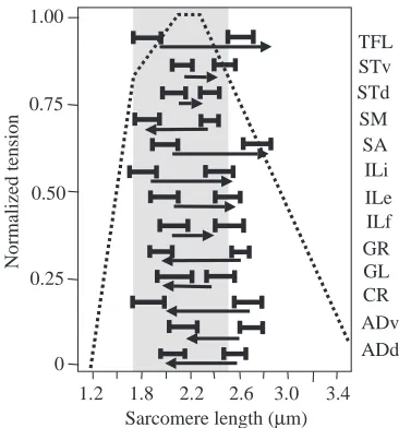
Because the hindlimb model reproduced the MTC moment arms from the test position, it could be used to predict sarcomere and fascicle lengths at different limb configurations. To test whether the model accurately predicted sarcomere lengths in experimental frogs and accounted for simultaneous changes in hip and knee angles, we measured sarcomere lengths at the starting and take-off positions of a jump in six frogs. We then placed the hindlimb model at these same two positions and determined what the predicted sarcomere lengths would be for each muscle. Data for experimental frogs (± 1 S.D.) and data predicted by the hindlimb model (solid horizontal arrows) are shown in Fig. 6. The arrow tail marks the predicted starting sarcomere length and the arrow head marks the predicted final sarcomere length. For most muscles (11/13), the model predictions lay within ± 1 S.D. of the mean values measured in the group of six frogs (standard deviations ranged from 0.10 to 0.25µm).

The sarcomere length predictions for CR, TFL and ILF lay outside ± 1 S.D. of the experimental means. The CR predictions may be affected by the fact that CR is highly pinnate (20–25 °) and the CR muscle model did not account for pennation angle changes with MTC length change or rigor contraction. Thus, our predictions of CR sarcomere length at

Table 2. Force-generating properties of the proximal hindlimb

muscles of Rana pipiens

Pennation Maximum

Mass angle PCSA force

Muscle (g) (degrees) (mm2_{) (N)}

ADd 0.108±0.01 0 6.93 1.89 ADv 0.113±0.01 5 8.22 2.24 CR 0.581±0.03 20 51.96 14.19

GL 0.195±0.02 0 14.28 3.9

GR 0.356±0.02 0 23.66 6.46 ILf 0.06±0.01 10 5.62 1.53

ILe 0.04±0.01 10 9.88 2.7

ILi 0.06±0.01 0 5.96 1.63

SA 0.075±0.01 0 3.67 1.01

SM 0.345±0.02 0 17.61 4.81

STd 0.047±0 15 5.53 1.51

STv 0.051±0 15 5.35 1.46

TFL 0.035±0.01 0 4.35 1.19

Muscle mass, pennation angle, and physiological cross-sectional area (PCSA) were measured for 13 hindlimb muscles in each of six frogs. The maximum force, or maximum isometric contractile tension, was estimated for each muscle (see Materials and methods).

SM, semimembranosus; GR, gracilus major; ADd and ADv, adductor magnus dorsal and ventral heads; CR, cruralis; GL, gluteus magnus; STv and STd, semitendinosus ventral and dorsal heads; ILf, iliofibularis; ILe, iliacus externus; ILi, iliacus internus; SA, sartorius; TFL, tensor fascia latae.

the take-off position were longer (by approximately 8–14 %) than sarcomere lengths measured experimentally. In contrast to pennation angle effects, TFL and ILF predictions may instead be affected by the fact that both muscles have a high in-series connective tissue length/muscle fiber length ratio (2.0–3.0) and these muscle models may not have adequately captured the in-series connective tissue properties (e.g. either the exponential stress/strain relationship or strain at maximum tetanic tension). Thus, model predictions were longer (by approximately 5–12 %) than sarcomere lengths measured experimentally. It will be necessary to perform sensitivity analyses to see how inaccuracies in modeling CR, TFL and ILF sarcomere lengths affect the dynamic behavior of the model and whether better models should be used, e.g. that account for pennation angle changes and muscle-specific connective tissue properties.

In Fig. 6, the classic isometric force/length curve (for SA; Gordon et al., 1966) is overlaid on the sarcomere length measurements to provide a general indication of where on the curve each of these muscles might operate during jumping. In general, most of the muscles appeared to operate over a range of sarcomere lengths where at least 80 % of the maximum contractile force could be produced. Nonetheless, it is important to stress that, because sarcomere measurements were performed under static conditions, in the absence of any tendon recoiling effects and velocity-dependent reductions in contractile force, the operating ranges reflect static ranges only and might be substantially different from ranges during jumping.

Architectural properties

We measured the muscle mass, pennation angle and PCSA SM

GR

ADd

GL CR

TFL

A

B

Hip extensors Knee extensors

for each of the 13 proximal muscles of the frog hindlimb in a total of six frogs. The data are shown in Table 2.

Static muscle functions

We constructed three-dimensional force fields to describe the multi-joint effects of muscle contraction. Force fields were constructed by placing the ankle of the model at a range of positions and maximally activating each musculotendon actuator at each position. The maximum contractile force of the actuator was calculated on the basis of a simulation of a fixed-end contraction (see Materials and methods). The static joint moments and the peak force produced at the ankle were calculated. The peak forces at each limb position were then plotted in the form of a three-dimensional force field. Each force field was normalized to the maximum force within the field to compare the fields produced by muscles with different

tension-generating capabilities (e.g. CR generated four times the force of ADd).

Fig. 7A shows muscle force fields for the three primary hip extensors (SM, top row; GR, middle row; ADd, bottom row). The left column shows a top view. The right column shows a side view. Each vector represents the peak force exerted by the ankle (against a virtual force sensor) at that particular limb position. If the limb were suddenly freed to move, the force vector would represent the initial direction in which the ankle would be accelerated. In three-dimensional space, there will be six forcing functions along which the limb could be accelerated: elevation and depression, caudal and rostral, and medial and lateral. The top view (left column) captures the caudal–rostral and medial–lateral forcing functions, and the side view (right column) captures the caudal–rostral and elevation–depression forcing functions.

ILi

ILe

ADv

SA

ST

ILf

A

B

C

Hip flexors Hip adductors

Knee flexors _{Fig. 8. Three-dimensional force fields produced by the monoarticular}

Examination of the top and side views for the hip extensor force fields in Fig. 7A shows that each muscle was multifunctional in terms of the six forcing functions. SM functions to elevate, caudally direct and medially direct the limb, with the balance of forcing functions changing across limb positions. ADd functions mainly to depress, caudally direct and medially direct the limb, with the balance of functions changing across positions. GR functions mainly to direct the limb caudally and medially and to bring the limb to the horizontal plane. Of these muscles, GR will have the largest effect on accelerating the ankle. GR produced a maximum ankle force of 0.74 N that was 1.37 times greater than that produced by SM (0.54 N) even though GR only produced a maximum contractile force that was 1.07 times greater than that produced by SM. This enhanced effect was because GR produced substantial hip and knee moments while SM produced only a very small knee moment.

Fig. 7B shows muscle force fields for the triceps group of muscles (CR, top row; GL, middle row; TFL, bottom row). These muscles were also multifunctional, and the balance of forcing functions was configuration-dependent. CR functions mainly to direct the limb laterally and rostrally. At elevated positions, CR elevated the limb and at depressed positions CR depressed the limb. GL functions mainly to elevate the limb. At rostral workspace positions, GL functions to direct the limb laterally when the ankle is held at low levels (due to hip adduction) and to direct the limb rostrally when the ankle is held at high levels (due to hip abduction). TFL functions mainly to direct the limb rostrally and laterally, and to elevate it. Because of the sarcomere/limb configuration relationship of TFL, this muscle produced little force at the ankle in the most rostral positions. Of these muscles, CR will have the largest effect on accelerating the limb. CR produced a maximum force of 0.90 N at the ankle compared with 0.39 N for GL and 0.15 N for TFL.

Fig. 8A shows muscle force fields for the two monoarticular hip flexors (ILi, top row; ILe, bottom row). ILi functions mainly to direct and elevate the limb rostrally, with a stronger elevator effect at caudal workspace positions. ILe functions to elevate the limb at mid to caudal positions, to direct the limb rostrally at rostral workspace positions and to depress the limb at elevated positions in the rostral workspace. The depressor function of ILe was due to a shift from producing an abduction moment at the hip to producing an adduction moment in combination with a small internal rotation moment at these rostral positions.

Fig. 8B shows muscle force fields for two hip adductor muscles (Adv, top row; SA, bottom row). ADv functions mainly to depress the limb and to direct it caudally and medially. SA functions mainly to depress the limb, but as opposed to ADv, to direct it rostrally. Thus, both muscles were multifunctional, and the balance of forcing functions was configuration-dependent. SA was particulary effective at directing the ankle rostrally at rostral (i.e. flexed) limb positions.

Fig. 8C shows muscle force fields for ST (combined

activation of STv and STd) and ILf. ST (top row) functions mainly to direct the limb medially. ILf functions mainly to elevate the limb. ILf exhibited an interesting bifunctionalily. At the lowest level in the limb’s workspace, ILf directed the limb caudally (i.e. acted to extend the ankle away from the body), while at the highest levels ILf directed the limb rostrally (i.e. acted to flex the ankle towards the body).

Discussion

This study quantified and developed the initial musculotendon subsystem of a biomechanical model of the frog Rana pipiens. The anatomical properties of 13 proximal muscles of the hindlimb were measured experimentally and implemented into actuators that formed the musculotendon subsystem of the model. The interaction between the musculotendon subsystem and a joint subsystem previously described by Kargo et al. (2002) reproduced experimentally measured changes in sarcomere length and moment arm across a wide range of limb configurations. Our model therefore captured the integrative (passive) behavior of the pelvis/hindlimb system of real frogs. The good fit between the model and the experimental data allowed us to use the model to estimate the maximum isometric forces that the muscles produce at different limb positions, to determine muscle force fields and to predict MTC length trajectories during specific motor behaviors (see below and Fig. 9). This set of analyses showed that frog hindlimb muscles have multiple functions with respect to accelerating the hindlimb in space and with respect to how muscles might function during specific motor tasks.

proximal muscle acts to accelerate the hindlimb from a large range of configurations.

The main finding of using the force field approach was that each hindlimb muscle was multifunctional with respect to its static, whole-limb effects. We described muscle function with respect to six forcing functions (see also Loeb et al., 2000). The six forcing functions were related to the six (extrinsic) directions in which the ankle could be accelerated (or forces applied to an object) in three-dimensional space. In the present study, we described the extrinsic directions as elevation and depression of the ankle within the gravitational plane, caudal and rostral movement of the ankle along the long axis of the frog, and medial and lateral movement of the ankle within the horizontal plane. At a single limb position, all muscles produced forces that had two primary vector components (i.e.

forcing functions), but most often all three vector components were substantial. Interestingly, the balance of forcing functions changed dramatically across the workspace of the hindlimb for nearly every muscle, e.g. a muscle that primarily directed the limb rostrally at one position might primarily elevate the limb at a different position. These configuration-dependent changes in muscle effects are likely to have a great impact on motor pattern selection and on the utilization of feedback to adjust motor patterns initiated from different starting configurations (see, for example, Kargo and Giszter, 2000b).

The multifunctional effects described above resulted from three fundamental properties of the hindlimb musculoskeletal system. First, each proximal limb muscle exhibited at least three moment arms about the hip (flexion–extension, internal–external rotation, abduction–adduction) and most Proximal limb k

ine

ma

ti

cs

Muscle force vector Ankle velocity vector

B

250 500 –1.0

–0.6 –0.2 0.2 0.6 1.0

A

Time (ms)

D

C

D

o

t

p

ro

d

u

ct

,

m

u

sc

le

f

or

ce

• a

nk

le

v

elo

ci

ty

0 0 250 500 0 250 500 0 50 100

Time (ms) Time (ms) Time (ms)

muscles exhibited a fourth moment arm about the flexion–extension axis of the knee. Importantly, the moment arms about a single joint axis changed with rotation about that axis and with rotations about adjacent joint axes (see Figs 3, 4). Thus, the ratio of moment arms exhibited by a muscle was configuration-dependent. In addition to moment arm variations, sarcomere lengths and therefore tension-producing capabilities changed with limb configuration. Thus, the balance and absolute magnitude of joint moments produced by a muscle were configuration-dependent, which has previously been noted in human studies (Friden and Lieber, 2000; Pandy, 1999). Finally, the Jacobian matrix, which determines how joint moments are transmitted through a multi-jointed limb to a point of contact with the environment or an object, is configuration-dependent (Tsai, 1999). Because of this, the forcing functions produced by a constant set of joint moments will depend on limb configuration (Mussa-Ivaldi et al., 1985). It is important to stress that we did not quantify the dynamic effects of muscle contraction in the present study. In theory, if the ankle were a point mass in a frictionless, gravity-less environment, the vectors comprising each muscle force field would represent the trajectory along which the ankle would be accelerated by muscle contraction. However, free limb trajectories are more complicated because of limb inertia, dynamic mechanical effects arising from multi-segmental motion, passive forces arising from stretched and shortened connective tissue structures and sensory feedback effects (Zajac, 1993; Crago, 2000). In addition, passive mechanical effects arising from motion of the large astragalus/calcaneus and foot segments in the frog are likely to have a large effect on the ankle trajectory. Nonetheless, force-field descriptions might provide some insight into muscle function that is complementary to functions observed with other experimental methods. For example, measurements of in vivo muscle length and force trajectories during specific behaviors showed that muscles function as motors, brakes, springs or struts in the context of the types of contraction performed, i.e. shortening, lengthening, lengthening/shortening and isometric contractions respectively (for a review, see Dickinson et al., 2000). In the following, we show how force-field descriptions might relate muscle function in terms of contraction type during specific behaviors to muscle function in terms of multi-joint limb effects.

Anatomically realistic models can be used to predict the length changes and contraction types of MTCs during specific behaviors when the kinematics and motor patterns for these behaviors are known (Arnold et al., 2000; Delp et al., 1998; Hoy et al., 1990). For example, when we moved our model through the swimming kinematic cycle described by Peters et al. (1996) and activated SM at experimentally determined times (Kamel et al., 1996; Gillis and Biewener, 2000), the SM musculotendon complex shortened during its period of activation and therefore functioned as a motor.

SM function can also be described in a more global sense. Specifically, the ankle force vector produced by SM contraction (small black arrow in Fig. 9A, lower panel) pointed

in the same direction as the velocity of the ankle during extension (gray arrow). The dot product between these two vectors at every time point during the swim cycle indicates that SM is activated mainly when it supports ankle acceleration (top panel of Fig. 9A; dot product more than 0.75). In contrast to muscle motors, muscle springs or brakes appear to produce forces at the ankle that are at 180 ° to the ongoing ankle velocity (dot product less than –0.75). For example, when we moved the model through a hindlimb wiping cycle and activated CR at experimental times (Kargo and Giszter, 2000a,b), CR produced forces that initially opposed and then supported ankle acceleration, which is consistent with a spring-like function (see Fig. 9B). Also, when we moved the model through a defensive kicking cycle and activated SA at experimental times (D’Avella et al., 2000), SA produced forces that opposed the entire extension phase, which is consistent with a braking function (see Fig. 9C).

Finally, some muscles might not be easily classified as motor, spring or brake. For example, when we moved the model through the jump extension phase (Kargo et al., 2002) and activated ST throughout, ST produced forces that acted neither to accelerate nor to decelerate the body. This was determined by calculating force directions generated by ST at the tip of the astragalus segment since this is the center of pressure for much of jumping (Calow and Alexander, 1973). We calculated the dot product of the ST force vectors with the (inverted) ground reaction force vectors published by Calow and Alexander (1973). ST forces were oriented at 90 ° to the forces applied to the ground. Therefore, ST was not helping to drive the astragalus into the ground but instead was acting in less obvious ways, e.g. redistributing moments or finely tuning the ground reaction force.