A computational fluid dynamics study of tadpole swimming

Tadpoles are traditionally considered to be inefficient swimmers compared with teleost fishes (Romer, 1966; Dudley et al. 1991); indeed, several characteristics of these amphibian larvae contribute to this impression. The abrupt transition from their globose bodies to their laterally compressed tails makes tadpoles seem less ‘streamlined’ than fishes (Videler, 1993). Tadpoles wobble: their snouts oscillate greatly when they swim, even in a straight line (Wassersug and Hoff, 1985). Such large lateral deflections certainly enhance the impression of mechanically inefficient locomotion. However, measurement of propulsive efficiency suggests that the mechanical efficiency of tadpoles may be almost as high as that of teleost fishes, such as salmonids (Wassersug, 1989). It is, in fact, not clear what the relatively simple shape of tadpoles means to their ability to swim or to their cost of locomotion.

Undulatory swimming by aquatic vertebrates is accomplished by propagating a traveling wave down the body to the tip of the tail. Undulatory swimmers cover a wide range of Reynolds numbers, from approximately 102_{for tadpoles up} to approximately 108_{for the most rapid cetaceans. Undulatory} swimming is the most effective movement for swimming propulsion and is employed by a large number of aquatic animals. Several excellent analyses by Lighthill (1971), Wu (1971a,b,c) and Newman (1973) have been developed for

modeling undulatory swimming in aquatic vertebrates. These analyses are based on inviscid potential flow theory. They have revealed many key points of undulatory propulsion, but still fail to address important subjects related to viscous flow during swimming, including separation, boundary layer and/or vortex production. Much is still unknown regarding the behavior of this unsteady viscous flow that could be of importance to undulatory propulsion.

A long-standing goal in fluid mechanics, and the key to understanding the importance of viscous fluid phenomena in estimating the propulsive efficiency of swimming animals, is solving the incompressible Navier–Stokes equations for unsteady flow.

In this paper, we describe a computational fluid dynamic (CFD) method developed by Liu (1995a,b). We apply this CFD method to a series of real biological problems involving flows around undulatory swimming animals.

The biological problems we address all concern the shape and locomotion of tadpoles. The tadpole is a good model organism for application of our CFD methods. First, the basic kinematics of locomotion in anuran larvae is well established (Wassersug and Hoff, 1985; Wassersug, 1989), which means that empirical data are available to describe precisely the form of the propulsive wave during undulatory swimming. Second, JEB0232

The hydrodynamics and undulating propulsion of tadpoles were studied using a newly developed two-dimensional computational fluid dynamics (CFD) modeling method. The mechanism of thrust generation associated with the flow patterns during swimming is discussed. Our CFD analysis shows that the kinematics of tadpoles is specifically matched to their special shape and produces a jet-stream propulsion with high propulsive efficiency, as high as that achieved by teleost fishes. Investigation of the effect of Reynolds number indicates that the Froude efficiency increases with increasing Reynolds number with no ceiling in generating the jet-stream propulsion. Further

studies using tadpole- and fish-shaped models with hindlimbs added to their body profiles reveal that the tadpole shape – a globose head with a tapered tail and hindlimbs at the base of the tail – allows tadpoles, but not fish, to develop hindlimbs with very little handicap on propulsion. The shapes and kinematics of tadpoles appear to be specially adapted to the requirement of these organisms to transform into frogs.

Key words: CFD (computational fluid dynamics), jet-stream propulsion, kinematics, swimming, metamorphosis, tadpoles, fish, locomotion.

Summary

A COMPUTATIONAL FLUID DYNAMICS STUDY OF TADPOLE SWIMMING

HAO LIU1, RICHARD J. WASSERSUG2 ANDKEIJI KAWACHI3

1_{Kawachi Millibioflight Project, ERATO, JRDC, Park Building 3F, 4-7-6 Komaba, Meguro-Ku, Tokyo, Japan,}

2_{Department of Anatomy and Neurobiology, Dalhousie University, Halifax, Nova Scotia, Canada, B3H 4H7 and}

3_{Research Center for Advanced Science and Technology, The University of Tokyo, 4-6-1 Komaba, Meguro-Ku,}

Tokyo, Japan

Accepted 29 February 1996

the common head–bodies of tadpoles are of a spheroidal shape that does not deform with locomotion, while tadpole tails are laterally compressed and tapered to a point. As a consequence of their overall simplistic morphology, a two-dimensional transverse section through a tadpole changes little in shape as one moves more dorsally or ventrally from the midplane of the body. Although our analyses to date are limited to two dimensions, we believe that this two-dimensional analysis provides interesting results and that this is an appropriate starting place towards the development of a truly realistic model of swimming in aquatic vertebrates.

We use our CFD analysis to examine the efficiency of tadpole locomotion. In addition, we address a series of other biological questions regarding tadpole morphology. (1) How costly is locomotion for tadpoles swimming with their unique kinematics compared with fishes? (2) Why do hindlimbs on tadpoles develop where they do, in the crease between the head–body and the tail? (3) Does fluid dynamics constrain tadpoles to a relatively small size?

The conclusions that emerge from these analyses are that tadpole locomotion is uniquely suited for their morphology and that the premetamorphic morphology of anurans is directly linked to their obligatory requirement to develop hindlimbs and transform into frogs.

Materials and methods

Unsteady solution to the Navier–Stokes equations In this study, we aimed to resolve viscous flow around an undulating creature. Unsteady solutions to the incompressible Navier–Stokes (N–S) equations are a key to understanding such highly unsteady fluid phenomena. We describe a computational system based on a method of two-dimensional N–S solving developed by Liu (1995a), which can be directly applied to realistic biological problems.

The nondimensionalized Navier–Stokes equations in the conservative form of x,y momentum and mass, if transformed into a generalized curvilinear coordinate system with a moving boundary, can be rewritten in an integral form as:

where

In the third equation of mass conservation, a time derivative of pressure is artificially added to the equation of continuity, with a positive parameter b. Vector q consists of two velocity

components of (u, v) and a pressure term p. Term S(t) expresses the area of a cell (i, j) constructed by four grid points, and l(t) are its four edges with unit outward normal vectors of

n=(nx, ny). Subscripts x and y denote derivatives with respect to x and y, and Re is the Reynolds number. To analyse the moving computational object of an undulating swimmer that continuously deforms, a body-fitted (boundary-fitted) mesh system that regenerates with time is introduced. This leads to a contribution from grid velocity Vg=(ug, vg) into the

governing equations.

The above governing equations are discretized using the finite volume method and are solved in a time-accurate manner, using the pseudo-compressibility technique (Chorin, 1958). A third-upwind differencing scheme is used to compute the convective term in an ultimate conservative difference scheme (Van Leer, 1977), and the viscous term is evaluated by a Gauss integration using the finite volume method. An implicit factorization approximate method, based on the Euler implicit scheme, is used for the discretization of the time derivative. In the time-accurate formulation, the time derivatives of the velocity components in the momentum equations are differenced using a first-order, two-point, backward-difference formula. To satisfy the equation of continuity at each physical time step, subiteration is also introduced, considering the artificial compressibility relationship.

For the two-dimensional modeling of an undulating object, the moving body may have three basic motions: translation, rigid rotation and flexible deformation. The translating motion can be replaced completely by introducing inertial forces into the momentum equations explicitly in a fixed coordinate system. For the rotating and deforming motions, however, this becomes quite difficult, which is why a moving mesh system is introduced. Since our goal is to compute unsteady flow around the undulating body, a method of regenerating grids fitting the deforming body surface at each time step with the outside boundary fixed is employed.

Kinematics of swimming

We base our kinematics on the bullfrog tadpole Rana catesbeiana, whose tadpoles are generalized pond-dwelling larvae with gross morphology and locomotor behavior similar to that of most tadpoles. The kinematics for undulatory swimming used in the present analyses is based on the straight locomotion of a Rana catesbeiana larva with a total length of 4.7 cm (Wassersug and Hoff, 1985).

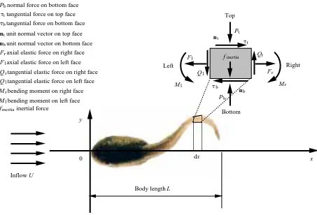
We first define the static geometry of our computational object by digitizing the shape of the Rana catesbeiana tadpole from a top-view picture (Fig. 1). An offset for grid generation, as illustrated in Fig. 2A, is then constructed using a spline interpolation technique, after appropriate smoothing. To ‘swim’ our tadpole, we created a sinusoidal function which sends a lateral wave propagating down the tadpole towards the tail tip. The wave is of the form:

(2) hi(x,t) = ai(x)sin 2p  − ,

    x l t T       . , , , ,

q = F = G =

2vy 0 uy+ vx v2_{+ p}

bv

vu

Gv=−

Fv=−

1 Re uy+ vx

0 2ux uv

bu

u2_{+ p} v p u 1 Re                                                   (1)

qdS + [(F + Fv)nx+ (G + Gv)ny−qVgn] dl = 0 ,

­

­t S(t)

⌠ 

where ai(x) represents amplitude, l is wavelength, T is period, hi(x,t) is the center line, t is time and x is the coordinate in the x-direction. By defining a reduced frequency of k =

(2pfL)/(2U) = (pL)/(TU), where L represents body length, f is

frequency and U is forward speed, we can obtain a simplified form of equation 2:

Subscript i denotes the grid points on the center line. Equation 3 for lateral motion is very compact, yet coincidentally similar to one developed by Videler (1993) for swimming fishes. Videler, however, developed his formula using the first three, odd Fourier terms, but pointed out that the contributions of the higher frequencies, even the third and the fifth, were marginal. Amplitudes of ai(x) are given by using the spline interpolation from five original maximum amplitudes along the length (L) of the tadpole: at the snout (x=0.0L, a=0.05L), at the otic capsule (x=0.19L, a=0.005L), at the base of tail (x=0.384L, a=0.04L), at the mid tail (x=0.692L, a=0.1L) and at the tail tip (x=1.0L, a=0.2L). These values are taken directly from Fig. 4 in Wassersug and Hoff (1985). The reduced frequency is

evaluated from a plot of forward velocity against tail-beat frequency in the same paper. The overall propulsive wavelength is taken as 0.87L, on the basis of empirical data of 0.87±0.1L (Wassersug and Hoff, 1985). Three normal swimming speeds of 1.5 L s21_{, 5 L s}21_{and 8 L s}21_{are selected} with corresponding frequencies of 4.7 s21_{, 9.2 s}21 _and 13.2 s21_{, resulting in Reynolds numbers of 2.1310}3_{, 7.2310}3 and 1.13104_{, respectively.}

Evaluation of thrust, power and Froude efficiency The Navier–Stokes equations, once solved, can give both micro and macro information on the flow field. Local flow patterns, no matter where they are (as long as they are inside the computational domain), can be described and visualized with the information generated on velocity and pressure at discretized grid points or cell-centers. Furthermore, integrated quantities, such as thrust, lift, etc., can be evaluated using the distributions of pressure and shear stress on the deforming body’s surface. To obtain these values, we make two assumptions: (1) the object is an elongated body with body length unchanged during swimming and (2) undulation is purely a lateral compressive motion. Kinematic tracings of swimming tadpoles in Wassersug and Hoff (1985) confirm hi(x,t) = ai(x)sin 2p  −2kt .

    x l       (3) Body length L 0 y Top Left Pt P Fl

Ql Fr

Qr M Ml Inflow U finertia tt tb nt nb Bottom dx normal force on top face

b normal force on bottom face

tangential force on top face

b tangential force on bottom face

unit normal vector on top face unit normal vector on bottom face axial elastic force on right face axial elastic force on left face

Qr tangential elastic force on right face Ql tangential elastic force on left face Mr bending moment on right face Ml bending moment on left face

inertia inertial force

Right b r P P t t n n F F f r l b t t t x

A

B

1.13e+₀₀

8.47e-01 5.65e-01 2.82e-01 0.00e+₀₀

these assumptions. With these caveats, we can now define the force-related quantities.

As illustrated in Fig. 1, two components of the force (Fx, Fy) acting on the body surface (Fbody) can be evaluated by

integrating the projection of pressure and shear stress in the x and y directions, respectively. As we see in equation 1, the present N–S solver builds a flux of both convective and viscous terms on the body surface at each cell, which means a force acting towards the direction of water flow. Therefore, summation of this opposite force over the whole body gives just the forward and lateral forces as follows:

Here, the third component Q comes from the equation of mass conservation, the third component of equation 1. Thus, thrust can be defined as 2Fx. Note that the contributions of both pressure and stresses are included in the present definition. On the basis of the previous analysis, we define the bending moment at an arbitrary point (xM, 0) on the center line as:

The power required for undulating swimming, i.e. the work done per unit time, can be considered as a summation of work done by inertial forces and by hydrodynamic forces containing pressure and stresses on the body surface, such that:

where ile and ite represent the leading edge (the head) and trailing edge (the tail tip), respectively, r is water density and Ai(x) is the area of section i on the center line. Any contribution of bending moment is neglected here.

To define the Froude efficiency (propeller efficiency), i.e. the rate of effective work done, for assessing the performance of an undulating swimmer, attention is paid to the instantaneous features of both thrust and power as described above. Considering the undulating object overall to be a propeller, we define our Froude efficiency Feff in a time-averaged manner (in one cycle), such that:

(7)

Feff= .

Thrustave×U Powerave

(6) Fyih˙i(x,t) , Fyv

=

^

body

i

^

ile Power =

$

Fyh˙(x,t)

≈

−

−

$

⌠  ⌡

L

0

rA(x)h˙(x,t)h¨(x,t)dx

rAi(x)h˙i(x,t)h¨i(x,t)Dxi

(5) [Fyi(xi−xM)] .

Fy(x−xM)≈

^

i Moment =

$

(4)

Fbody= Fy =−

Q Fx

    

    

[(F + Fv)nx+ (G + Gv)ny] .

(Fluxinviscid+ Fluxviscous)

^

body

i

=−

^

i

C

Here Thrustave is net thrust including the force due to skin friction. Note that, using the above definition, swimming at constant velocity will result in zero Froude efficiency. We suggest a method of assessing the performance in such a case by comparing the power output.

In order to make comparisons among different species, we define the thrust, the moment and the power in nondimensionalized forms as:

Here Sbodyexpresses the surface area of the object.

Results and discussion

Computational validation

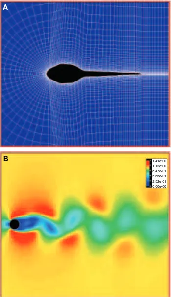
A variety of validation tests were undertaken (Liu, 1995a,b) to assess the reliability of results using this CFD method. We give an example of flow around a circular cylinder at a Reynolds number of 105 in Fig. 2B. The von Karman vortex street in the wake is captured well by our simulation when compared with reported experimental results (Van Dyke, 1982). Similarly, our Strouhal number St of 0.156 is also in good agreement with many experimental results, such as those of Tritton (1959) and Kovasznay (1949), who report values very close to 0.16. Other CFD results on unsteady flow behind an accelerated flat plate and around a pitching foil were also in reasonable agreement with previously reported values.

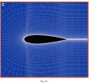
Generally, the quality of grids, including grid number, orthogonality, smoothing and minimum spacing, affects the CFD results. To achieve high resolution of the flow in the wake and to make grids easily fit the moving boundary of our object, a C-type grid topology, as illustrated in Fig. 2A, was chosen. We tested two grid systems: one was 199341 (199 grids in the streamwise direction and 41 grids in the direction vertical to the body surface) with 50 grids in the wake, the other 163341 with 30 grids in the wake. For both grid systems, the minimum grid spacing (dmin) normal to and adjacent to the body surface was controlled using an experimental formula of dmin=0.1/√−Re. Grids were clustered to the solid wall in order to resolve viscous flow inside the boundary layer. Grids were also clustered at the leading and trailing edges because of steep pressure divergence there. The computational domain was limited to a region around the body with a radius for the outside open boundary of 6 L. Since the higher reduced frequency of 5.843 (corresponding to a swimming speed of 5 L s21_{, see above) leads to a} nondimensionalized period of approximately 0.54, a physical time increment dt of 0.01 was taken. All the computations

were carried out using an HP Apollo 9000 series workstation (model 755).

The tadpole swimming mechanism

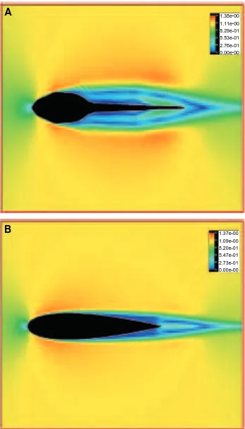
We first analyzed steady flows around a tadpole with its tail kept straight (at Re=7200), to assess dead drag (Fig. 3A). The non-streamlined shape of the tadpole produces a large dead drag coefficient of 0.115, compared with the value of 0.067 given by the more typically fish-shaped body of the NACA0020 hydrofoil, as illustrated in Fig. 3B. For the tadpole, there is a pair of large-scale vortices visible at the posterior tail, and strong back flows over the tail tip up to the head–body, resulting in a large region of thick boundary-layer separation over the tail. This produces a greater pressure component for the drag coefficient, but at the same time reduces the friction component for the drag coefficient. At the Re examined here, frictional drag coefficient is equal to 0.0084 for the tadpole compared with a value of 0.0235 for the fish-like body.

A representative speed of 5 L s21_{(corresponding to a Re of} 7200), a speed at which a Rana catesbeiana larva normally swims, was chosen for investigating the flows around the undulatory swimming tadpole. The flow pattern, visualized in a velocity fringe manner in Fig. 4, shows a completely different pattern from the steady case shown in Fig. 3A. In the wake, it is clear how the vortices released at the end of every stroke to the left and to the right gradually increase in size, but decrease in strength due to viscous dissipation (Fig. 4). Note that the vortex sheet looks very similar to the famous von Karman vortices, as in Fig. 2B, but shows opposite rotation. The flow between the vortices is accelerated backwards, forming a jet-stream, very similar to the wake pattern photographed by Wassersug and Hoff (1985) of a Rana pipiens tadpole swimming through a thin layer of milk. The tadpole gains an opposite forward force from the momentum in this jet. This is the source of the thrust of jet-stream propulsion in undulating swimmers. Furthermore, focusing attention on the near-wall flows, we see that the large-scale vortices observed in the steady, straight-tail situation (Fig. 3A) disappear. In addition, the region with the separated thick boundary layer in the steady case reduces to a very small region at the base of the tail when the tail is undulating. Contrary to expectation, the boundary layer along the posterior tail becomes thinner during undulatory swimming in comparison with the steady case. We believe that this is because viscosity makes fluid particles on the body surface have the same velocity as the oscillating body. This, in turn, leads to the local flow being accelerated and oscillating in correspondence with the undulating body. Considering the law of energy conservation, fluid near the wall usually gains kinetic energy from the mechanically oscillating body. This means that the momentum being lost due to the viscous dissipation inside the boundary layer is instantaneously supplied from this mechanical oscillation, which contributes to the production of the jet-stream in the wake.

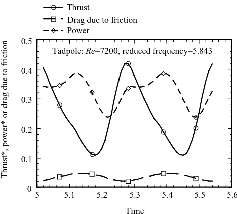
Hysteresis of thrust, power and drag due to friction are plotted against time in Fig. 5. Velocity profiles and iso-(8)

Thrust* = Thrust , Gr_U2_S

body

(9)

CM= ,

Moment Gr_U2_S

bodyL (10) Power* = and . Power Gr_U3_S

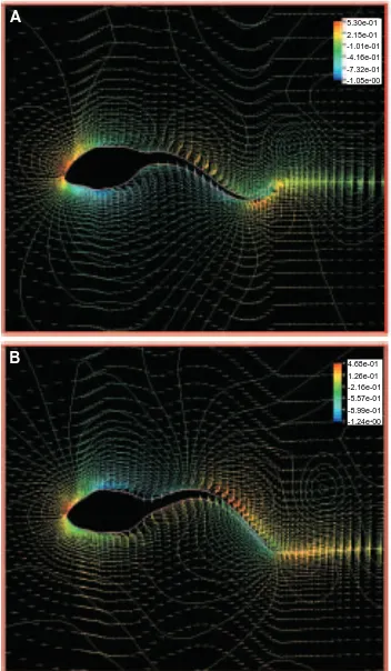
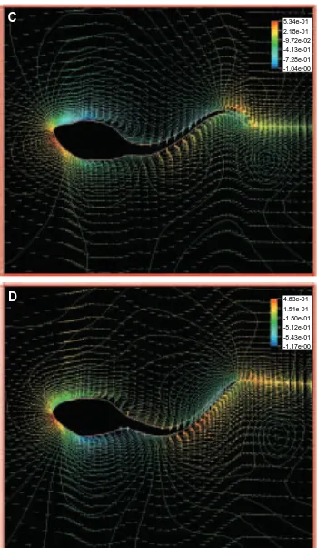
pressure distributions at four moments, t=5.18 (≈0T), t=5.28 (≈T/5), t=5.45 (≈T/2) and t=5.55 (≈4T/5), during one cycle are shown in Fig. 6A–D, respectively. The instantaneous thrust coefficient reaches its maximum with a value of 0.41 twice in

each cycle because of the symmetrical undulating movement of the tail to the left and right. The maxima occur when the tail takes an arched form (C-shaped) with a maximum angle of incidence (equivalent to an angle of attack) and a maximum

A

B

1.38e+₀₀

1.11e+₀₀

8.29e-01 5.53e-01 2.76e-01 0.00e+₀₀

1.37e+₀₀

1.09e+₀₀

8.20e-01 5.47e-01 2.73e-01 0.00e+₀₀

area to push water backwards immediately following the position of the tail tip at which it has its maximum amplitude. The iso-pressure contours show that both the upper (pushed by positive pressure) and lower (sucked by negative pressure) sides of the arched tail contribute to thrust generation. At the two thrust maxima, the frictional drag coefficient reaches a minimum while the power curve reaches a value of 0.33 (Fig. 5). Since the thrust has a higher value than the power at these two points, the tadpole can achieve a very high instantaneous propeller efficiency (equation 7) of 124.2 %. In contrast, the S-shaped tail, at the two points where it occurs in each cycle, leads to a minimum thrust with a value of 0.11, but a larger friction drag coefficient of 0.042 (maximum friction drag coefficient = 0.047). At this point, the power curve has a value of 0.30, almost three times the instantaneous thrust, clearly handicapping its instantaneous propeller efficiency (36.3 %).

Note that the variation with time of the thrust curve gives a positive mean value of 0.26. This indicates that a tadpole, if swimming at the same speed (5 L s21_{) and with the same} kinematics, would be accelerating rather than swimming at a steady speed. Using equation 7 as explained above, we calculated the propeller efficiency or Froude efficiency from the averaged thrust (0.26) and the mean power (0.32), leading to a value of 82.2 % at a Reynolds number of 7200. Wassersug (1985) reported a very similar value of 83 % from empirical kinematic data, using the formula Feff=120.5(12U/Vc), where Vc is the velocity of the traveling wave, U is the forward swimming speed and Feffis Froude efficiency.

We also calculated the Strouhal number (St) for vortices in

the wake, determined by tail-beat frequency (f), forward speed (U) and the width of vortices in the wake (AM), i.e. St=2AMf/U, yielding a value of 0.72. A series of studies on

1.97e+₀₀

1.57e+₀₀

1.18e+₀₀

7.86e-01 3.93e-01 0.00e+₀₀

Fig. 4. Flow pattern around an undulatory swimming tadpole at a Reynolds number of 7200. The frame of reference is fixed on the moving swimmer. Note that a jet-stream is clearly detected in the wake, gradually increasing in width, but decreasing in strength. Also, the large-scale vortices that were visible in the computation of steady flow around a straight-tailed tadpole (Fig. 3A) disappear, reducing to a small separated region at the base of the tail. Additionally, the boundary layer at the posterior tail becomes thinner.

Fig. 5. Hysteresis of thrust, power and drag due to friction plotted against time at a Reynolds number of 7200. Variation during nearly two periods is shown within an interval of dimensionless computational time from 5.0 to 5.8. Each variable is a nondimensionalized coefficient as described in Materials and methods. Both the thrust and the drag due to friction reach peak values twice during each cycle because of the symmetrical left and right deflection of the tail.

0 0.1 0.2 0.3 0.4 0.5

5 5.1 5.2 5.3 5.4 5.5 5.6 Thrust

Drag due to friction Power

Thrust*, power* or drag due to friction

Time

the optimum swimming of teleost fishes by Triantafyllou et al. (1995) shows that fishes normally generate a jet-stream of high propulsive efficiency (greater than 80 %) with a Strouhal number ranging from 0.2 to 0.4, half that obtained here for tadpoles. The magnitude of the vortex width is dominated by the maximum amplitude of the undulating motion at the tail tip. A comparison of tail-beat frequency versus specific swimming speed among fishes and tadpoles in Fig. 12 of Wassersug and Hoff (1985) showed a tight regression line for tadpoles and fishes. A review of fish kinematics (Table 6.1 in Videler, 1993) indicated that maximum amplitudes at the tail tip lie at around 0.1L for most fishes, which is approximately half that reported by Wassersug and Hoff (1985) for tadpoles. Hence, the higher tail amplitude (almost double that of carangiform fish such as salmon and trout) will contribute to the higher Strouhal number for tadpoles. We believe that tadpoles manage to swim efficiently in comparison with teleost fishes, but using very different kinematics. Below, we suggest that these high-amplitude kinematics fit the special shape of tadpoles and help them to achieve jet-stream propulsion effectively.

In addition, the drag coefficient due to friction on swimming tadpoles varies from 0.021 to 0.047 with a mean value of 0.032. This value is almost four times that calculated for the dead drag coefficient (0.0084) and is mainly because the velocity gradient at the body surface, inside the boundary layer, becomes steeper due to local accelerated motion, especially at the posterior tail. Therefore, an undulating body or, generally speaking, an oscillating body relative to a non-undulating body will have a reduced drag due to pressure or may even generate greater thrust, but has an increased friction resistance. As the skin friction drag is significantly affected both by the Reynolds number and by the undulating motion, any analysis that fails to consider the behavior of the unsteady boundary layer cannot accurately estimate thrust, power and propeller efficiency during swimming.

Interactions between the head–body and the tail As noted above, tadpoles use specific kinematics matched to their particular shape and size for jet-stream propulsion. In this regard, we have assumed that tadpoles do not produce thrust effectively by using their tails alone. The head–body also takes an active part in generating thrust, which requires an interaction of flows between the head–body and the tail.

To illustrate how the kinematics of locomotion for tadpoles is closely matched to their shape, we computed the flows around a fish-shaped body (a NACA0020 hydrofoil) oscillating with the same kinematics as the tadpole. Specifically, we ‘allowed’ this fish-shaped object to have large-amplitude lateral deflections at the snout, similar to the rostral wobble seen in swimming tadpoles. The result is illustrated in Fig. 7. The hydrofoil that we used had the same maximum thickness (0.2L) as the tadpole. Although a jet-stream flow pattern similar to that around tadpoles is established, the streamlined hydrofoil retains a thin boundary layer without separation over the whole body. As discussed previously, this will lead to

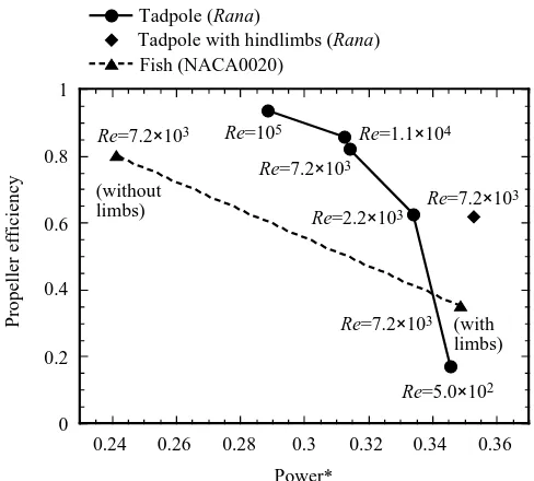
increased friction drag. The averaged value of the frictional drag coefficient was 0.050, or nearly 1.5 times the value for the tadpole swimming in the same mode. Mean thrust was 0.19, i.e. only 73 % of the thrust produced by the tadpole. The fish-shaped body, however, required very low power (0.24) for swimming, so that it still achieved a high propeller efficiency of 0.80 (Fig. 8). Note that the propeller efficiency for the fish-like body swimming in the tadpole kinematic mode is slightly less than that for the tadpole. We conclude that, with the high oscillations at the snout and tail tip that characterize tadpole kinematics, tadpoles can actually produce jet-stream thrust with a high propeller efficiency, similar to that produced by a fish-like body swimming in the same manner. Thus, we cannot derive a reasonable estimate of the efficiency of undulatory swimming merely by considering the tail as a propeller isolated from the body.

Furthermore, it should be noted that the power requirement is greater for the tadpole than for the fish, which is consistent with the ecology of this organism. As inhabitants of small bodies of water, tadpoles do not swim continuously for long distances or at high speeds (Wassersug, 1989). Perhaps the broad conclusion to be drawn from this analysis is that the popular view of what is either a streamlined shape or an efficient kinematic pattern can be very misleading. While neither its globose shape nor the wobble in its swimming movement gives the tadpole the subjective appearance of efficient locomotion, both features function in concert. The kinematics of a tadpole is closely linked to its premetamorphic morphology. All told, the tadpole is an efficient undulatory swimmer.

Implications for metamorphosis

5.30e-01 2.15e-01 -1.01e-01 -4.16e-01 -7.32e-01 -1.05e+₀₀

A

B

1.26e-01 -2.16e-01 -5.57e-01 -8.99e-01 -1.24e+₀₀

fast extend and adduct their hindlimbs. This reduces the height of their knees and should help them to retain relatively high propeller efficiency values.

‘Hindlimbs’ were also added to our model of the undulatory fish-shaped body. These ‘limbs’ were the same size and shape as the ‘knees’ of our tadpole and were placed at the same

C

D

5.34e-01 2.18e-01 -9.72e-02 -4.13e-01 -7.28e-01 -1.04e+₀₀

4.83e-01 1.51e-01 -1.80e-01 -5.12e-01 -8.43e-01 -1.17e+₀₀

distance along the rostral–caudal axis as in the tadpoles (Fig. 10). CFD anlysis shows a flow pattern very different from that around the tadpole (compare with Fig. 9). A separated region is observed near the added limbs, which seriously affects both the local boundary layers and the pressure distributions. This results in a sharp reduction of the propeller efficiency to 0.35 (Fig. 8). Hence, addition of these ‘limbs’ had major detrimental effects on flow around the fish compared with the tadpole.

The overall implication of these simulations of tadpole and

fish with limbs added is that the shape and kinematics of tadpoles are as much driven by the tadpoles’ requirement to grow hindlimbs and to transform into frogs as by any aspect of larval locomotion. Fish do not transform into limbed creatures, and their body form and kinematics are not adapted to the development of hindlimbs and feet.

Reynolds number effect

Because all known tadpoles are small (<23 cm total length; Emerson, 1988) and they swim at relatively low Re (<105_{), we} suspected that fluid dynamic factors might constrain organisms that were shaped like and swam like tadpoles from efficient locomotion at high Reynolds numbers. We tested this hypothesis by modeling the flow around tadpoles swimming at

Fig. 7. Flow pattern around an undulating fish-shaped object swimming using a tadpole kinematic mode, i.e. with large lateral oscillations at the snout, at a Reynolds number Re of 7200. Over the whole body, the boundary layer is thinner than for the tadpole at the same Re, swimming with the same propulsive wave form (see Fig. 4).

0 0.2 0.4 0.6 0.8 1

0.24 0.26 0.28 0.3 0.32 0.34 0.36 Tadpole (Rana)

Tadpole with hindlimbs (Rana) Fish (NACA0020)

Propeller efficiency

Power*

Re=105 _Re=1.1×104

Re=7.2×103

Re=2.2×103 Re=7.2×10 3

Re=5.0×102

Re=7.2×103 _(with limbs)

Re=7.2×103

(without limbs)

Fig. 8. Variation of propeller Froude efficiency versus power with changing Reynolds number plotted for a tadpole (Rana catesbeiana) and a fish-like body (NACA0020 hydrofoil). The line with five circles indicates the change in output power with Froude efficiency at the Reynolds numbers shown. The curve is parabolic, with a tendency for power to decrease with increasing Re. At a realistic tadpole speed (Re=7200), the CFD analysis yields a value of Froude efficiency of 0.822. The diamond symbol indicates the value for a swimming tadpole with developing hindlimbs at the base of the tail. The two triangles indicate values for a fish swimming in the tadpole kinematic mode (Re=7200), with and without hindlimbs. Although the power requirement of this fish model is smaller than that of the tadpole (about 0.25) and it produces a high propeller efficiency, similar to that for the tadpole, the presence of protruding hindlimbs seriously handicaps a fish, with a sharp reduction in propeller efficiency to 0.35 and an increase in power requirement to 0.35.

2.03e+₀₀

1.63e+₀₀

1.22e+₀₀

Re values up to 105_{. We investigated how the jet-stream} propulsion varies with increasing Re, i.e. the effect of Reynolds number, by undertaking a series of computations at Re values

of 2.13103_{, 7.2310}3 _{and 1.1310}4 _{(at which the Rana} catesbeiana larva normally swims) and at two additional Re values of 53102 _{and 10}5_{. The resulting flow patterns at Re of}

1.98e+₀₀

1.58e+₀₀

1.19e+₀₀

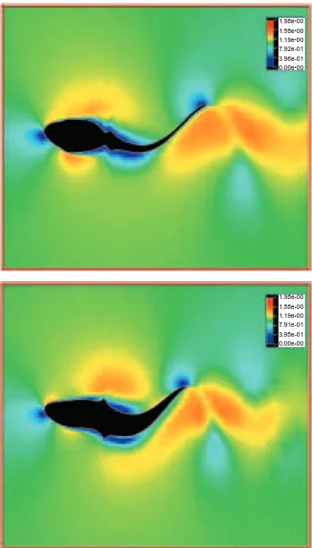
7.92e-01 3.96e-01 0.00e+₀₀

1.98e+₀₀

1.58e+₀₀

1.19e+₀₀

7.91e-01 3.95e-01 0.00e+₀₀

Fig. 9. Flow pattern around an undulatory swimming tadpole with hindlimbs, at a Reynolds number of 7200. Only a slight deformation of the boundary layer at the base of the tail is detected in comparison with a tadpole without protruding hindlimbs (see Fig. 4).

A

B

2.01e+₀₀

1.61e+₀₀

1.20e+₀₀

8.03e-01 4.01e-01 0.00e+₀₀

2.03e+₀₀

1.63e+₀₀

1.22e+₀₀

8.14e-01 4.07e-01 0.00e+₀₀

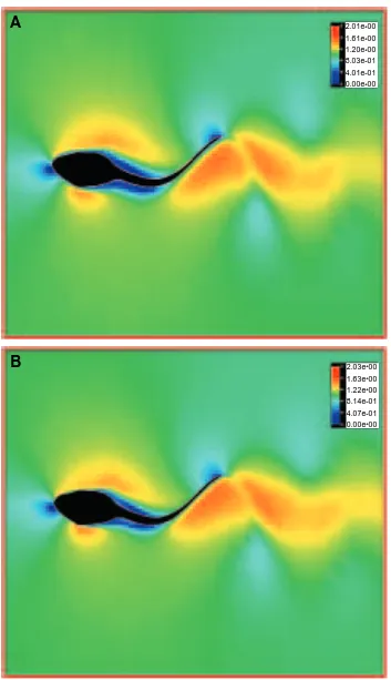
Fig. 11. Flow patterns around three undulatory swimming tadpoles at Reynolds numbers of 2.13103_{(A), 1.1310}4_{(B) and 10}5 _(C).

2.13103_{, 1.1310}4 _{and 10}5 _{are shown in Fig. 11A–C. Similar} jet-stream patterns, as well as the separated region at the base of tail, are seen for all the Reynolds numbers. Also, close-up views of near-wall flows show that the velocity gradients inside the viscous boundary layers, especially at the posterior tail, become steeper due to local undulating motions. This should, as described above, lead to an increase in the drag due to friction. An overall tendency to reduce the drag due to friction, however, is observed in our CFD analysis with increasing Reynolds number. Notice that the quantity of the viscous term, as shown in the N–S equations (equation 1), which is determined by the inverse Reynolds number and the velocity gradient, ordinarily decreases with increasing Reynolds number. This is because the increase in the velocity gradient with increasing Reynolds number is usually less than the increase in Reynolds number alone. In this regard, the skin friction drag during swimming is mainly affected by two key factors, the undulating motion and the Reynolds number. Overall, our CFD analysis for tadpoles indicated a tendency for a reduction in frictional drag with increasing Reynolds number.

Jet-stream propulsion shows a tendency to achieve high efficiency at high Reynolds numbers. In other words, the energy exchange between the mechanically oscillating body and the local fluid flow should become more efficient with increasing Reynolds number. A plot of propeller efficiency against power at different Reynolds numbers for the tadpole (Fig. 8) follows a parabolic curve. In fact, we achieved a

propulsive efficiency of 0.93 at a Re of 105 _{using the} assumption of the body undergoing sinusoidal swimming motion and without taking into consideration either transition or turbulence. We suggest that a giant tadpole the size of a dolphin swimming at a Re of 105_{, using the present specific} kinematics, would still be capable of effectively producing the jet-stream. In contrast, the current kinematics rapidly result in a reduction in the propeller efficiency of the tadpole when the Reynolds number decreases to 53102_{. This is consistent with} the observation that the kinematics of tadpole swimming changes greatly at slow swimming speeds when Reynolds numbers are very low, as illustrated in Fig. 3 of Wassersug and Hoff (1985).

We conclude that fluid dynamics alone does not constrain tadpoles to small size or low velocity. Rather, physiological (e.g. muscle contraction velocity; Lutz and Rome, 1994) and/or ecological (e.g. predation risks; Werner, 1986) factors confine tadpoles to living at low Reynolds numbers.

Our results establish the power of CFD to explain the design of living organisms. In our present study, CFD models have helped us to understand the specific undulatory mechanism of tadpoles compared with fishes. Through these computational methods, we have been able to perform ‘experiments’, such as making fish swim in a tadpole mode, which have never been performed with unconstrained living animals. Such computational experiments have also made it possible to compare different undulatory swimming methods over a much larger Re range than that occurring in nature. Our CFD models

C

1.61e+₀₀

1.21e+₀₀

8.04e-01 4.02e-01 0.00e+₀₀

provide insight into how different shapes and sizes interact with kinematics and why different swimmers are built in any particular way. A CFD three-dimensional analysis of undulatory locomotion would further enhance the realism of our model and is our next task.

List of symbols

AM maximum width of vortices in a wake A(x) area of section x on the center line

(nondimensional)

ai(x) amplitude at point i on the center line (nondimensional)

CM bending moment coefficient (nondimensional)

dt time increment

Fbody force acting on body surface

Feff Froude efficiency

Fx, Fy components of force acting on body surface (nondimensional)

f frequency (Hz)

hi(x,t) center line of a tadpole (nondimensional) h˙(x,t) velocity component in the y-direction of segment

x at time t (nondimensional)

h¨(x,t) acceleration component in the y-direction of segment x at time t (nondimensional)

k reduced frequency

L body length (nondimensional) l(t) four edges of a cell (i, j) at time t

(nondimensional)

n=(nx, ny) unit outward normal vector of a cell (i, j) p pressure (nondimensional)

Powerave time-averaged power coefficient (nondimensional)

Power* power coefficient (nondimensional)

Q residual of the equation of mass conservation

Re Reynolds number

S surface area

Sbody surface area of the object

S(t) area of a cell (i, j) at time t (nondimensional)

St Strouhal number

T period (nondimensional) Thrustave time-averaged thrust coefficient

(nondimensional)

Thrust* thrust coefficient (nondimensional)

t physical time

U forward swimming speed (nondimensional) u, v velocity components (nondimensional) Vc velocity of traveling wave (nondimensional)

Vg=(ug, vg) grid velocity (nondimensional)

xM center of bending moment (nondimensional) b any positive parameter

dmin minimum grid spacing adjacent to the body surface

l wavelength (nondimensional)

r water density

t pseudo (artificial) time (nondimensional)

We thank Ms Susan Hall, Dr Shigeru Sunada and Dr Takeshi Ohnuki for their technical assitance and valuable comments. We extend our thanks to Dr Robert Dudley for his critical comments. This research was supported by the Research Development Corporation of Japan and the Natural Science and Engineering Research Council of Canada.

References

CHORIN, A. J. (1958). Numerical solutions of the Navier–Stokes

equations. Math. Comput. 22, 745–762.

DUDLEY, R., KINGV. A. ANDWASSERSUG, R. J. (1991). Implications

of shape and metamorphosis for drag forces on a generalized pond tadpole. Copeia 1991, 252–257.

EMERSON, S. B. (1988). The giant tadpole of Pseudis paradoxa. Biol.

J. Linn. Soc. 34, 93–104.

KOVASZNAY, L. S. G. (1949). Hot-wire investigation of the wake behind cylinders at low Reynolds numbers. Proc. R. Soc. Lond. A

198, 174–190.

LIGHTHILL, M. J. (1971). Large-amplitude elongated-body theory of

fish locomotion. Proc. R. Soc. Lond. B 179, 125–132.

LIU, H. (1995a). Unsteady solutions to the incompressible

Navier–Stokes equations with the pseudo-compressibility method.

Proceedings of the 1995 ASME/JSME Fluids Engineering Annual, FED 215, 105–121.

LIU, H. (1995b). Computation of unsteady flows around a

rigid/flexible oscillating body with the MUSCL method.

Proceedings of the International Conference on Computational Engineering Science 1, 817–832.

LUTZ, G. J. ANDROME, L. C. (1994). Built for jumping: the design of

the frog muscular system. Science 263, 370–372.

NEWMAN, J. N. (1973). The force on a slender fish-like body J. Fluid Mech. 58, 689–702.

ROMER, A. S. (1966). Vertebrate Paleontology. Chicago: University

of Chicago Press.

TRIANTAFYLLOU, G. S., TRIANTAFYLLOU, M. S. ANDGROSENBAUGH, M.

A. (1995). Optimal thrust development in oscillating foils with application to fish propulsion. J. Fluids Structure 7, 205–224. TRITTON, D. J. (1959). Experiments on the flow past a circular cylinder

at low Reynolds numbers. J. Fluid Mech. 6, 547–567.

VANDYKE, M. (1982). An Album of Fluid Motion. The Parabolic Press. VANLEER, B. (1977). Toward the ultimate conservative differencing

scheme. IV. A new approach to numerical convection. J. comp.

Physics 23, 276–299.

VIDELER, J. J. (1993). Fish Swimming. London: Chapman & Hall. WASSERSUG, R. (1989). Locomotion in amphibian larvae (or ‘Why

aren’t tadpoles built like fishes?’). Am. Zool. 29, 65–84.

WASSERSUG, R. ANDHOFF, K. (1985). The kinematics of swimming

in anuran larvae. J. exp. Biol. 119, 1–30.

WERNER, E. E. (1986). Amphibian metamorphosis: growth rate,

predation risk, and the optimal size at transformation. Am . Nat.

128, 319–341.

WU, T. Y. (1971a). Hydrodynamics of swimming propulsion. Part 1. Swimming of a two-dimensional flexible plate at variable forward speeds in an inviscid fluid. J. Fluid Mech. 46, 337–355.

WU, T. Y. (1971b). Hydrodynamics of swimming propulsion. Part 2.

Some optimum shape problems. J. Fluid Mech. 46, 521–544. WU, T. Y. (1971c). Hydrodynamics of swimming propulsion. Part 3.

Swimming and optimum movements of slender fish with side fins.