Minimization of electro mechanical interaction with posicast strategies for more electric aircraft applications

Minimization of Electro-Mechanical Interaction with

Posicast Strategies for More-Electric Aircraft

Applications

C. Ahumada1_{, S. Garvey}2_{, T. Yang}1_{, P. Kulsangcharoen}1_{, P. Wheeler}1_{, H. Morvan}2

Departments of 1_{Electrical and Electronic Engineering,} 2_{Mechanical, Materials and Manufacturing Engineering}

Faculty of Engineering, University of Nottingham Nottingham, United Kingdom

[email protected]

Abstract— This paper studies strategies to minimize the electromechanical interaction (EMI) within aircraft power systems. With the growth of electrical power on-board aircraft, the interaction between the electrical systems and the engine core will become significant. The behaviour of electrical loads (on/off, transient etc.) will have significant impacts on the engine shaft, such as producing transient vibrations, creating stability problems and reducing the efficiency etc. To avoid these problems, an advanced electrical power management system (PMS) is required. This paper introduces novel loading methods for PMS applications to minimize the interactions between electrical and mechanical systems. The strategies, referred as Single Level Multi-edge Switching Loads (SLME), Multilevel Loading (MLL), and Multi-load Single Level Multi-edge Switching Loads (MSLME) are developed based on the Posicast method. An insight look of the developed technique has been studied using the zero-pole root locus. It is demonstrated that the excited poles in the system are cancelled by the addition of zeros, and thus supressed the EMI vibrations.

Keywords— Transient, Electromechanical Interaction

I. INTRODUCTION

The More Electric Aircraft (MEA) has become one of the main trends for future aircraft technologies. Many functions, which were driven by pneumatic, mechanical and hydraulic power in conventional aircraft, are being gradually replaced by electrical devices. The increased use of novel electrical loads also gives rise to the electrical power extracted from the engine. In some cases, such as taxiing period when the engine is at the idle mode, the electrical power may account for more than 50% of the total engine power [1]. A higher electrical power system allows having more flexible systems and a higher range of applications, but also introduces new challenges. One of these challenges is the interaction between the electrical and mechanical power system.

In conventional aircraft, the electrical system has a small impact on the mechanical system, due to the difference in sizes: the electrical system is small compared to the mechanical one, and therefore the short term changes of it do not affect the mechanical system [2]. However, with a higher electrical power rating, the connection of electrical loads produces transients vibrations which, as it has been shown in [3], are transferred to the mechanical system, stressing and weakening the shaft [4],

[5]. The maximum vibration allowed by the shaft depends on two material properties, i.e. the ultimate stress and the endurance stress [6].

• Ultimate stress: Maximum peak magnitude of an oscillation that the material can withstand.

• Endurance stress: Maximum duration of an oscillation that the material can withstand.

In order to reduce the vibrations due to the EMI and consequently extend the material lifecycle, the transient period needs to be minimized. The aim of the paper is to minimize the EMI between the electrical power system and the shaft of the generator of an aircraft system.

This paper proposed a PMS that uses strategies based on the Posicast compensation method [7], [8]. In the PMS, the electrical loads are categorized as Time Critical Loads and Time Non-critical Loads with respect to its connection properties. For each type of loads, the PMS will apply different strategies.

The rest of the paper is organized as follows: in section II the EMI system in study is modelled and analysed. Section III presents the natural frequencies relationship with the vibrations and the Posicast compensator. After, section IV introduces strategies to minimize the vibrations produced by the EMI. Finally, in sections V and VI, a strategy to identify parameters of the system and the conclusions are presented.

II. THE ELECTROMECHANICAL SYSTEM

This section presents the EMI system of an aircraft: in section A, the model is introduced; in section B, the parameters of the system are defined; and in section C the response to an electrical load connection is shown.

A. Modelling of the System

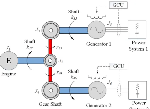
The connections between the engine and the power system of an aircraft can be represented by Fig. 1 [4]. The engine, represented by an E, is connected to two generators. Each generator has a control unit (GCU) and supplies power to the electrical power system. The modelling of the EMI system is divided into the mechanical and electrical parts.

Fig. 1. Electromechanical interaction system.

1) Mechanical System Modelling

The mechanical system can be represented as a lumped mass system with three key parameters i.e. the inertias, the stiffness and the damping factor [9]. The EMI system in study (Fig. 1), consists of 6 inertias ( , = 1,2, … , 6) including the engine, the gear box and generator rotors. These inertias are connected through shafts (horizontal connections) or a gear shaft (vertical connections). Each shaft connection has an associated stiffness and damping, given by and , with and the sub-index of the related inertias being connected. In the case of the gear shaft connection, a gear ratio is given by .

To model the system, the torques acting over each inertia are modelled. In (1) the torque equation for inertia 1 is shown, with the torque applied by the engine, and the torque being used by the shaft. The torque on the shaft connecting inertias 1 and 2 can be calculated by (2), with , , and , the position, speed and acceleration of inertia .

= − (1)

= ( − ) + ( − ) ₍₂₎

Repeating the same proceeding done for inertia 1 on the rest of the system, the lumped mass system of the EMI is found as shown in (3), with the rotational angles of each inertia as a state, and the inertia ( ), stiffness ( ) and damping ( ) matrices defined according to the connections described. The input of the system is made out of the torques , , and , which are being applied by the electrical system and are modelled in section 2. The matrices and vectors values are presented in (4).

+ + = ₍₃₎

=

0 0 0 0 0

0 0 0 0 0

0 0 0 0 0

0 0 0 0 0

0 0 0 0 0

0 0 0 0 0

=

− 0 0 0 0

− 0 0 0 0

0 0 0 − 0

0 0 0 0 −

0 0 − 0 0

0 0 0 − 0

₍₄₎

=

− 0 0 0 0

− 0 0 0 0

0 0 0 − 0

0 0 0 0 −

0 0 − 0 0

0 0 0 − 0

=

0 0 0 0 0 0 0 0 0 0 0

0 − 0

0 0 − =

It is important to notice that the lumped mass model in (3) does not consider the effect of the gear box J2, which relates the

speed from inertias 3 ( ) and 4 ( ) to the speed of inertia 2 ( ), as shown in (5). Considering this relationship, the system from (3) can be reduced to a system of 4 states ( , , , ) using the transformation matrix of (6). In (7) the reduced matrices of the system are shown.

=

= (5)

=

1 0 0 0

0 1 0 0

0 0 0

0 0 0

0 0 1 0

0 0 0 1

(6)

= = = = = ′

(7)

2)Electrical System Modelling

The obtained lumped mass model is connected to the electrical one through the applied torques , and .

In this paper, the generator is modelled as a DC machine since from a control point of view, the control of a DC machine and an AC one is the same. Consequently, the electrical power system is modelled as a DC grid connected to a resistive load. Equations (8) and (9) show the torque of each machine and the voltage equation of the power system, with , the airgap torque of the generators, , the machines constant, , the current on each power system, , the terminal voltage of each generator, , and , the line parameters of the power systems, and , the voltage of the loads of each power system.

, = , , (8)

, = , , + , , + , (9)

Additionally, each generator has a GCU, which regulates the terminal voltage to be constant. Subsequently, an electrical load connection to the generator has a proportional impact on the torque of the generator, as presented in [3], [10]. For simplification, in this paper the electrical load connections will be represented as changes in the airgap torque of the generators , . As a result, to model the EMI only the value of the generators torque will be needed.

Secondly, the engine of the system is going to be modelled as torque , which value depends on the speed of the shaft ( = ). Its behaviour can be modelled by a lineal equation given by (10), in which and are constants.

3) System integration

The system integration is achieved by combining the mechanical model from (7) and the electrical one (8) and (10). First, the torques driven by the engine and the generator must be included in (7). The torques of generators are inputs of the system. On the other hand, the torque of the engine, depends on the speed of the shaft, hence its constant is added as a damping parameter to the matrix in the position (1,1), while the constant remains as an input of the system. The state space system given by (11).

= +

= (11)

Where:

= ₋ 0 ₋ = ₋ =

= 0 − 0 0 − 0 (12)

The states of the system are the rotational angles and the rotational speed of each inertia; the input are the torques applied by the generators and , and the constant associated with the engine torque . And the output is the torque connecting the shaft from inertia 4 to 6, = .

B. Parameter Definition

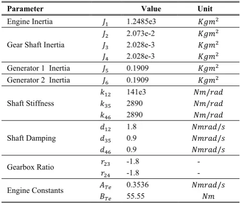
The system is designed to have two mechanical natural frequencies between 10 and 30Hz in order to represent the typical values of aircraft systems [4]. Moreover, as the engine is considered the ground of the system, its inertia value has to be at least 100 times the generator inertia. Table I shows the parameters that are going to be used for the rest of the paper. TABLE I.PARAMETERS OF THE ELECTROMECHANICAL SYSTEM.

Parameter Value Unit

Engine Inertia 1.2485e3

Gear Shaft Inertia

2.073e-2 2.028e-3 2.028e-3 Generator 1 Inertia 0.1909 Generator 2 Inertia 0.1909

Shaft Stiffness

141e3 /

2890 /

2890 /

Shaft Damping

1.8 /

0.9 /

0.9 /

Gearbox Ratio -1.8 -

-1.8 -

Engine Constants 0.3536 /

55.55

Using the values from Table I on the A matrix from (12), the natural frequencies and damping of the system are obtained:

• = 0 and = 1

• = 17.46 and = 0.017

• = 24.95 and = 0.022

• = 334.01 and = 0.049

C. Step Response of the System

To show the EMI, the system of (11) is analysed using MATLAB/Simulink software. A step load torque is applied to the generator and the torque transient is observed. Fig. 2 shows the response to a connection from 3 to 10Nm. The torque applied on the generator represents the connection of an electrical load (solid line), while the torque on the shaft (dashed line) shows the EMI of the system. It is observed that the connection of an electrical load generates transient vibrations on the shaft. Thus, there is an EMI and its effect must be studied.

Fig. 2. Step response of the system.

The next section will focus on development of strategies to eliminate these vibrations.

III. FREQUENCY CONCEPT

In order to eliminate the vibration due to EMI, first the relationship between load connection, and natural frequencies must be described. Secondly, the Posicast method that uses this relationship is introduced.

A. Effect of Natural Frequencies on Vibrations

For undamped and underdamped systems, as the one of the EMI of an aircraft, the complex conjugate poles , define the system vibration characteristics. These conjugate poles can be written as:

= − ± 1 − = − ± (13)

Where is the natural frequency, is the damped frequency, and is the damping ratio.

Moreover, the response ( ) of a system initially in equilibrium to an external excitation ( ) can be given by the Duhamel integral as shown in (14). Where ( ) is the system impulse response function [11], [12].

( ) = ( ) ( − ) (14)

From here, the algebraic analysis presented in [10] is followed. The response to a step connection at a time , ℎ( −

), is defined as the integral of a the impulse function,

( − ) . Moreover, following a modal approach [13],

the step response can be written as a function of step response modes, as shown in (15), where represents the kth _eigenvalue

and ℎ represents the coefficient of the step response associated with the eigenvalue .

Assuming that ( ) is a sequence of step excitations, such as ( ) = ∑ = , the response of the system can derived and presented in (16), where ( ) is the response of the system, and are the value and time of the pth _{step applied}

to the system, is the poles being excited, and ℎ is the associated step response [11].

( ) = ℎ + ℎ exp ( ( − )) (16)

In order to supress the vibrations of the related to , the steps applied to the system have to be orthogonal to the vibration characteristic. This condition is satisfied when (17) is solved.

real exp − = 0 ∀ > (17)

B. Posicast Compensator

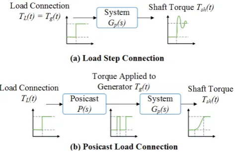
The solution of (17) was proposed in [7], [8] using the Posicast method. In Fig. 3(a), the transient response of the system after a step response is shown. While, in Fig. 3(b) the open loop Posicast compensator is used. Instead of using one single step excitation system, in Fig. 3(b) a series of step excitation signals are applied. By carefully choosing the excitation time and amplitude, the vibrations can be supressed.

Fig. 3. System diagram with and without Posicast compensator.

The Posicast compensator can be modelled as a series of delayed step connections as shown in (18), in which and represent the pth _{step connection value and the time of it.}

+ + ⋯ + + ⋯ + (18)

IV. STRATEGIES AND STABILITY ANALYSIS

In this section, a PMS that allows the cancelation of shaft vibrations due to electrical load transient is developed. The electrical loads of an aircraft are categorized into different types according to its operation characteristic. Different Posicast strategies will be applied according to the load type. A zero-pole root locus technique is used to explain the effect of the Posicast compensators on the overall system.

A. Aircraft Load Classification

The main loads in a MEA, given in [1], are shown in Table II. These loads can be separated into two groups: Time Critical and Time Non-critical Loads.

TABLE II.CLASSIFICATION OF LOADS ON AIRCRAFT SYSTEM

Time Critical Time Non-critical

Flight Control Surfaces (2-35kW) Fuel Pumps (10kW)

Landing Gear (5-70kW) Engine starting (200kW)

De-Icing (20kW) Cabin Air (4*70kW)

Time Critical Loads are the ones in which the connection time represents a crucial factor for its operation. For these loads is essential to have a precise connection time. An example is the case of the flight control surfaces or the landing gear, which cannot have a delay in their connection. On the other hand, Time Non-critical Loads are the ones for which an exact time connection is not a crucial factor for its operation. For example, the de-icing system and the air cabin can be connected and disconnected at any time during the flight. In particular, it was stated in [14], that the de-icing system must be part of the time on and off. This characteristic is the one that makes the de-icing system the perfect load to use on the PMS strategies, as it will be shown.

B. PMS Strategies

1)Time Non-critical Strategies

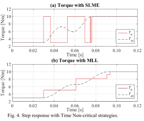
As there is no need of an exact connection time for a Time Non-critical Load, the PMS can apply the Posicast compensator directly to the load connection. For these cases, the Posicast based strategies Single Level Multi-edge Switching Loads (SLME) and Multi-level Loading (MLL) were introduced in [10]. SLME consists in connecting the load as a series of on/off pulses, as can be seen in (solid line) in Fig. 4 (a); while MLL, consists in connecting the load by a sequence of steps as shown in (solid line) in Fig. 4 (b).

To obtain the time instant and step values of the SLME and MLL strategies, the equations in (19) and (20) must be solved respectively. These equations are derived from (17) as presented in [10]. The subscript represents the natural frequency with which the equation is associated, and sub-index

, the number of the step connection.

The EMI system in this study has three non-zero natural frequencies ( = 17.46, 24.95, 334.01 ). In order to eliminate the vibrations, the SLME strategy will have 7 connection pulses . Moreover on the equation system = 0, and = ±1 for the odd and even step connections respectively. Therefore, the connection times − are the parameters that will be solved. On the other hand, MLL will have 4 connection steps , and the following constrains: = 0, and ∑ = 1. Hence, the values of the times − and the step values , , must be found.

of the strategies SLME and MLL allow suppression of the shaft vibrations due to electrical load connections.

cos( ) + ⋯ + cos

+ ⋯ + cos( ) = 0

sin( ) + ⋯ + sin

+ ⋯ + sin( ) = 0

(19)

cos( ) + ⋯ + cos

+ ⋯ + cos( ) = 0

sin( ) + ⋯ + sin

+ ⋯ + sin( ) = 0

(20)

Moreover, both strategies are applied in half of the periods of the natural frequencies, making the total loading time in the order of milliseconds. In addition, the SLME connection behaves as mechanical switches, which have a bounce in its connection. Radar and de-icing systems are examples of loads in which it can be applied. On the other hand, the MLL strategy is suggested for loads that do not need to be loaded to its full power at one single time instant. These loads can be multilevel converters fed drive systems or the ice protection systems.

Fig. 4. Step response with Time Non-critical strategies.

2) Time Critical Strategy

For Time Critical Loads, like flight control surfaces, to which a delay in the connection cannot be applied in order to avoid the vibrations produced by a step connection the PMS uses an auxiliary load. Auxiliary Loads are going to be Time Non-critical Loads that are already connected to the system, and to which a Posicast based strategy is going to be applied. The electrical power of the Time Non-critical Load must be higher than the one of the Time Critical Load being connected. An example of an auxiliary load is the de-icing system presented in [14] where is stated that the de-icing system is following an on-off-on pattern.

The strategy applied by the PMS to Time Critical Loads ( ) will consist in the pulsating connection and disconnection of an auxiliary load ( ) with the SLME strategy. Fig. 5(a) shows this approach. As can be seen, while the Time Critical Load ( in dashed line) is connected by step, the Auxiliary Load ( in dashed-dot line) is using the SLME method. In this

way, the total load applied on the generator ( = + ), shown in solid line in Fig. 5(a) and (b), is not a single step. This strategy will be called Multi-load Single Level Multi-edge Switching Loads (MSLME).

The equation system that needs to be solved to find the time connections of that allows eliminating the vibrations will include the connection time of and . As it was done for the Time Non-critical Loads, the equation system to find the step values and the time connections is derivate from (17) and shown in (21). For the system in study 6 connection pulses are going to be needed in order to supress the vibrations. Considering = 0 and the steps as a partial disconnection of the auxiliary load , which takes values = ± for the even and odd steps respectively, the variables that need to be solved are the times − and the value of the auxiliary load disconnection .

cos( ) + ⋯ + cos

+ cos( ) + cos( ) = 0

sin( ) + ⋯ + sin

+ sin( ) + sin( ) = 0

(21)

The system is solved in MATLAB with Opti Toolbox [15], and the system is tested in Simulink. Fig. 5 shows the results obtained for a Time Critical Load connection of 3Nm when the auxiliary load connected to the system is of 10Nm. As already stated in Fig. 5(a) the value of (dashed-dot line), (dashed line), and the total load applied to the generator (solid line) are shown. It is observed that, even though the critical load is connected as a step connection, the total torque applied to the generator is a series of pulses thanks to the Auxiliary Load. In Fig. 5(b) the total torque over the generator (solid line) and the shaft torque (dashed line) are presented. The total system transient shows the elimination of the vibrations compared to the step result of section II. C, which demonstrated the effectiveness of this loading pattern. This connection takes a maximum of half period of the system natural frequencies.

C. Root Locus Analysis

To understand the effect on the system of the introduced PMS strategies, zero-pole root locus of the system in each case is analysed.

The total transfer function of the system depends on the plant transfer function, , and the Posicast compensator transfer function, , as presented in (22). is obtained from the “A” matrix presented in section II.A, while is obtained from the Posicast representation given by (18), in which represents the step at a time . Thus, representing the time delays of the step connections by Padé of order 6, the transfer function is given as

( ) = ( ) ( ) (22)

Fig. 6 shows the poles of the system with the zeros added by the Posicast strategies. Fig. 6 (a) presents the poles (represented by x) of the plant while Fig.6 (b), (c) and (d) show the poles and zeros (represented by o) when the system is with the Posicast compensator. It can be seen, that the zeros from the Posicast compensator (added to the system by using the SLME, MLL, and MSLME methods) provides additional zeros which cancelled the poles in the original system. Thus the cancelled poles cannot be excited from input signals and thus suppress the mechanical vibrations in the system.

Fig. 6. Poles (shown by x) and zeros (shown by o) of the system.

V. PARAMETER IDENTIFICATION

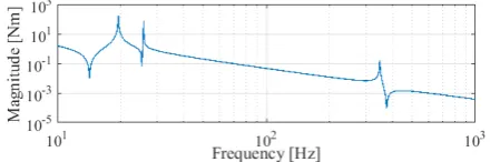
To identify the parameters of a real system, in particular the natural frequencies and damping ratios, the Fourier analysis to a step load response is done. In Fig. 7 is observed the Fourier transform obtained from the shaft response to a step load connection, which was presented in Fig. 2. It is observed that the frequencies of the system are 17.46, 24.95, and 334.01 Hz, which correspond to the frequency design values. Therefore, the Fourier analysis is a good identification system for EMI system.

Fig. 7. Fourier analysis of the vibration absorber case of the system in study.

VI. CONCLUSIONS

In new aircraft system due to higher power system EMI need to be analysed. This paper presented one of the effects of the EMI on aircraft systems, as well as a PMS that allows its solving.

The PMS consists of strategies that eliminate the vibrations produced on the generator shaft due to electrical load connections. It studies the cases of Time Critical and Time Non-critical Loads, and according to its characteristics applies one of the three Posicast based strategies: Single Level Multi-edge Switching Loads (SLME), Multi-level Loading (MLL), and Multi-load SLME (MSLME).

In order to eliminate the vibrations, the PMS uses strategies based on the timing of the load connection, for which the natural frequencies and damping ratio need to be know. For real systems, it was shown that Fourier analysis can be used for the identification of its values. Therefore, the PMS proposed presents a viable solution for the transient vibrations due to EMI.

REFERENCES

[1] P. W. Wheeler, J. C. Clare, A. Trentin, and S. Bozhko, “An overview of the more electrical aircraft,” Proc. Inst. Mech. Eng. Part G J. Aerosp. Eng., vol. 227, no. 4, pp. 578–585, Apr. 2013.

[2] T. Wu, S. Bozhko, G. Asher, P. Wheeler, and D. Thomas, “Fast Reduced Functional Models of Electromechanical Actuators for More-Electric Aircraft Power System Study,” in SAE Power Systems Conference, 2008, p. 12.

[3] C. Ahumada S., S. Garvey, T. Yang, and P. Wheeler, “Electric Load Impact over Shaft Connecting the Engine and Generator in More Electric Aircraft (MEA),” in SAE Technical Papers, in Press. [4] T. Feehally, I. Damian, and J. Apsley, “Analysis of

electro-mechanical interaction in aircraft generator systems,” IEEE Transactions on Industry Applications, vol. PP, no. 99. p. 1, 2016. [5] P. J. Norman, S. J. Galloway, G. M. Burt, D. R. Trainer, and M. Hirst,

“Transient analysis of the more-electric engine electrical power distribution network,” Power Electronics, Machines and Drives, 2008. PEMD 2008. 4th IET Conference on. pp. 681–685, 2008. [6] J. S. Joyce, T. Kulig, and D. Lambrecht, “Torsional Fatigue of

Turbine-Generator Shafts Caused by Different Electrical System Faults and Switching Operations,” Power Apparatus and Systems, IEEE Transactions on, vol. PAS-97, no. 5. pp. 1965–1977, 1978. [7] O. J. M. Smith, “Posicast Control of Damped Oscillatory Systems,”

Proceedings of the IRE, vol. 45, no. 9. pp. 1249–1255, 1957. [8] G. Tallman and O. Smith, “Analog study of dead-beat posicast

control,” IRE Transactions on Automatic Control, vol. 4, no. 1. pp. 14–21, 1958.

[9] C.-M. Ong, Dynamic Simulation of Electric Machinery: Using MATLAB/SIMULINK. Prentice Hall PTR, 1998.

[10] S. C. Ahumada, S. Garvey, T. Yang, P. Wheeler, and H. Morvan, “The importance of load pulse timing in aircraft generation,”

Electrical Machines and Systems (ICEMS), 2015 18th International Conference on. pp. 1339–1345, 2015.

[11] M. I. Friswell, J. E. T. Penny, S. D. Garvey, and A. W. Lees,

Dynamics of rotor machines. Cambridge University Press, 2010. [12] K. Veselić, Damped Oscillations of Linear Systems, 1st ed., vol.

2023. Berlin, Heidelberg: Springer Berlin Heidelberg, 2011. [13] C. W. de Silva, Vibration: Fundamentals and Practice, Second

Edition. CRC Press, 2011.

[14] E. W. Giloy, “An Electric Deicing System for Aircraft,” Transactions of the American Institute of Electrical Engineers, vol. 68, no. 2. pp. 1051–1057, 1949.

[15] J. Currie and D. I. Wilson, “OPTI: Lowering the Barrier Between Open Source Optimizers and the Industrial MATLAB User,” in