Loop oscillations in the corona

LOOP OSCILLATIONS IN THE CORONA

Lorna James

A Thesis Submitted for the Degree of MPhil

at the

University of St Andrews

2004

Full metadata for this item is available in

St Andrews Research Repository

at:

http://research-repository.st-andrews.ac.uk/

Please use this identifier to cite or link to this item:

http://hdl.handle.net/10023/12947

Loop Oscillations in the Corona

Loma James

-Lk/ 3a%'.AJ ' ' 'X'

y \

..

iJJ \ N /

A

Thesis submitted for the degree of Master of Philosophy

of the University of St Andrews

ProQuest Number: 10171059

All rights reserved

INFORMATION TO ALL USERS

The quality of this reproduction is dependent upon the quality of the copy submitted.

In the unlikely event that the author did not send a com plete manuscript and there are missing pages, these will be noted. Also, if material had to be removed,

a note will indicate the deletion.

uest

ProQuest 10171059

Published by ProQuest LLO (2017). Copyright of the Dissertation is held by the Author.

All rights reserved.

This work is protected against unauthorized copying under Title 17, United States C ode Microform Edition © ProQuest LLO.

ProQuest LLO.

789 East Eisenhower Parkway P.Q. Box 1346

Abstract

Magnetic loops in the Sun’s corona have been discovered to oscillate in a variety of modes. The oscillations are observed to exhibit strong damping. A number of theo­ ries have been put forward to explain the damping, including resonant absorption and phase mixing. Here we consider the modelling of loop oscillations, paying particular attention to two effects: gravity, and the addition of a chromospheric layer below the corona.

We develop an acoustic model of coronal loop oscillations and consider two ways of describing the effects of the gravitational stratification and the chromospheric lay­ ers, considering either two media separated by a discontinuous interface or a single medium with a sound speed that varies along the loop.

A dispersion relation for the two-layer isothermal atmosphere case is obtained and in­ vestigated numerically using a bisection code. On comparison with roots obtained for a single isothermal atmosphere, it was found that the effect of chromospheric footpoints on the period of a mode is slight.

However, the effect of gravity was found to be more notable, rising up to a twenty percent change in period when considering the longer observed loops. This result is of especial interest since gravity is often ignored by authors discussing loop oscillations.

Declaration

1. I, Lorna James, hereby certify that this thesis, which is approximately 16,000 words in length, has been written by me, that it is a record of work carried out by me and that it has not been submitted in any previous application for a higher degree.

d a te signature of candidate . ...

2. I was admitted as a research student in October 2001 and as a candidate for the degree of MPhil in July 2003; the higher study for which this is a record was carried out in the University of St Andrews between 2001 and 2004.

date ... signature of candidate .. ...

3. I hereby certify that the candidate has fulfilled the conditions of the Resolution and Regulations appropriate to the degree of MPhil in the University of St An­ drews and that the candidate is qualified to submit the thesis in application for that degree.

2 . i

date ; .y"( r.L .-frr.T. /. signature of supervisor

4. In submitting this thesis to the University of St Andrews I understand that I am giving permission for it to be made available for use in accordance with the regulations of the University Library for the time being in force, subject to any copyright vested in the work not being affected thereby. I also understand that the title and abstract will be published and that a copy of the work may be made and supplied to any bona fide library or reseaich worker.

Acknowledgements

Many thanks to my supervisor, Prof. Bernard Roberts, for helping me to finish this thesis and submit my Masters.

Thanks to all the friends in St Andrews and beyond who have always been there for me.

I gratefully acknowledge the love and support of my special honey, Francois-Xavier.

Finally a special thankyou must go to my family for the many supportive phone con­ versations throughout my postgraduate and undergraduate life.

Contents

1 O bservations o f loop oscillations 5

1.1 The S u n ... 5

1.2 How we observe... 7

1.3 Before T R A C E ... 8

1.4 After T R A C E ... 9

1.5 Damping ... 12

1.6 SUMER and slow w a v e s ... 14

2 M H D waves 16 2.1 MHD eq u atio n s... 16

2.2 Sound waves ... 17

2.3 Magnetic w a v e s... 19

2.4 Waves in a structured m e d iu m ... 23

2.5 Waves in a uniform m ed iu m ... 24

2.6 Waves at a magnetic in terface... 25

2.7 Waves in a magnetic s l a b ... 26

2.8 Waves in a magnetic flux tube ... 28

2.9 G r a v i t y ... 30

3 Coronal loop oscillation m od el 35 3.1 Coronal Loop m o d e l ...35

3.2 Case 1 - Isothermal atm o sp h ere...37

3.2.1 Dispersion re la tio n ... 37

3.2.2 An isolated m e d iu m ... 39

3.2.3 Shallow chromospheric la y e r... 40

3.2.4 Dimensionless dispersion re la tio n ... 43

3.3 Case 2 - Continuous sound s p e e d ...46

3.3.1 Confirming the Bessel re s u lt... 48

4 R esu lts 52

4.1 Effect of chromospheric l a y e r ... 52

4.1.1 Checking numerical m e th o d ... 52

4.1.2 Numerical re su lts ... : ... 54

4.2 Effect of g rav ity ... 56

4.3 Applying theory to SUMER d a t a ...60

5 C onclusion 65 5.1 Thesis summary ...65

5.2 The impact of a chromospheric l a y e r ...66

5.3 The impact of g r a v i t y ...66

5.4 Possible future w o r k ...66

A B ou ndary C ondition 67

B D im en sionless D ispersion R elation 70

C Solar Values 72

D Zeros of C ross-P rod ucts o f B essel F unctions 74

List of Figures

1.1 The layers of our Sun ... 5

1.2 The rise in tem perature above the solar s u rfa c e ... 6

1.3 Coronal loop observed by T R A C E ... 7

1.4 Spectrum of w avelengths... 7

1.5 Radio pulsations ... 8

1.6 Loop oscillations on 14 July 1998 ... 10

1.7 Damping of coronal lo o p ... 11

1.8 Histogram comparing TRACE and SUMER loops... 15

2.1 A travelling w a v e ... 18

2.2 Polar plots of magnetoacoustic w aves...21

2.3 Surface and body w a v e s ...22

2.4 Sausage and kink m o d e s...22

2.5 Equilibrium magnetic in te r fa c e ...25

2.6 Equilibrium magnetic s la b ...26

2.7 Dispersion plot for magnetic surface w aves...28

2.8 Wave modes in a magnetic cylinder... 29

3.1 Coronal loop m o d el... 35

3.2 Simplified coronal loop m o d e l... 36

3.3 Isolated s la b ... 39

3.4 Sketch of the dimensionless wave frequency for an isolated coro­ nal structure 45

3.5 Sketch of the period for an isolated coronal s tru c tu re ... 45

4.1 Dispersion plot for small h ...53

4.2 Dispersion diagram for small h ...54

4.3 Dispersion diagram for large h ...55

4.4 Impact of loop length on A rg ra v ity... 60

List of Tables

1.1 Properties of TRACE l o o p s ... 12

1.2 Properties of SUMER lo o p s ... 15

3.1 Bessel asymptotic s o lu tio n s ... 51

4.1 Comparison of wave frequency obtained numerically and analyt­ ically ...53

4.2 Effect of chromosphere on p e r io d ...56

4.3 Effect of gravity on p e rio d ... 59

4.4 SUMER waves compared to slow m o d e ... 61

Chapter 1

Observations of loop

oscillations

1.1 The Sun

Our Sun is a star like all the others in the night sky. One property that makes the Sun unique is its distance from us; it is one Astronomical Unit away, approx­ imately 1.5 X lO^^m (Priest 1982). The next closest star is Proxima Centauri at

a distance of 4.29 light years, which is 271000 times farther away from us than the Sun. The Sun therefore gives us a unique opportunity to study in depth the physics of a star.

Photosphere Chromosphere

onvec _Radiativo

Figure 1.1: The layers of the Sun. [1]

convection zone, energy is transm itted through overturning convective motions of the medium. These convective motions are observed at the solar surface as supergranules and granules.

The outer Sun consists of the photosphere, chromosphere and corona. The photosphere is thought of as the surface of the Sun as this is seen in normal light. Above the photosphere is the chromosphere. The corona is basically everything above the chromosphere spreading far out into space.

The corona is a very interesting medium with many puzzles still unan­ swered. A m ajor puzzle is that of its tem perature. The Sun’s tem perature gradually decreases from the core to the photosphere, dropping from 10^ K to 6000 K. But in the thin transition region between the chromosphere and the corona the tem perature rises abruptly to 2 x 10® K (see Figure 1.2).

1 Million

I

^ 100000

Photosphere Chromosphere Corona

I

I

1000

1000 1500

Height above convection zone (km)

500 2000 2500 3000

Figure 1.2: The rise in tem perature above the solar surface. [2]

Figure 1.3: A coronal loop photographed by TRACE on 12 September 2000. [3]

1.2 How we observe

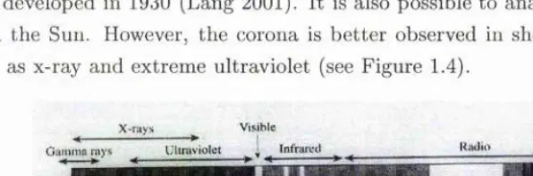
The corona is hard to observe from the E arth since the light from the photo­ sphere dominates. It can be viewed during eclipses when that light is blocked out by the Moon, and scientists have learnt to make their own artificial eclipses. Telescopes were modified to have a disk in the middle which would block out the main part of the Sun. Such instruments are called coronagraphs and were first developed in 1930 (Lang 2001). It is also possible to analyse radio signals from the Sun. However, the corona is better observed in shorter wavelengths such as x-ray and extreme ultraviolet (see Figure 1.4).

X-rays

Gamma rays

Visible L'lliaviolet i Infrared

10-^ 10" 10'-

Wavclciiglh (m)

Figure 1.4: The spectrum of wavelengths. (Lang 2001)

accelerated? SOHO has been successful in producing data for helioseismology, the study of the Sun’s interior by observing the oscillations of its surface. The m ajor instruments giving data for helioseismology are VIRGO, GOLF and MDI. VIRGO had the aim to determine the characteristics of long-wavelength global sound waves from irradiance variations (Frohlich 1995). GOLF had the aim to study the internal structure of the Sun by measuring the spectrum of global os­ cillations in low frequency ranges (Gabriel et al 1995). MDI provides scientists with magnetograms of the photosphere but it also detects modes of oscillation of the Sun and that data has been used to produce amazing spectrums of global oscillations (Scherrer et al 1995). Another im portant instrum ent on SOHO is SUMER (Solar Ultraviolet Measurements of Em itted Radiation) (Wilhelm et al 1995), a spectrometer (see section 1.6).

The spacecraft that has had the most impact on the study of oscillations of coronal loops is Transition Region And Coronal Explorer (TRACE). TRACE was launched in April 1998 and, with the help of filters to view different wave­ lengths, its aim was to study the connection between fine-scale magnetic fields and the associated plasma structures (Handy et al 1998). TRACE has high cadences, with a time-cadence of 10 seconds and a spatial resolution of 0.5 arc- seconds. This is much greater than SOHO which has a cadence of 30 seconds and a resolution of 2.5 arc-seconds.

1.3 Before TR A C E

Figure 1.5: Microphotometric tracing of radio pulsations observed on February 25, 1969, 09:55 UT, in the frequency range of i/ = 160 — 320 MHz at

the Utrecht radio observatory. Note that besides the fundamental mode of Pi « 3 s, there are also subharmonic pulse structures with periods of P2 ~ 1 s

visible. (Rosenberg 1970)

P = 0.5 — 5.0 seconds (see Figure 1.5) and was the first to put a name to them, calling them ‘radio pulsations’. It was not until later when more theoretical work was done (Roberts 1981a,b and Edwin and Roberts 1983) that a possible definition of oscillations observed by radio waves was suggested, Roberts, Edwin and Benz (1984) applied the theory of fast sausage MHD waves for a coronal plasma and used this to find the period.

Pfastsausage

where a is the loop radius, Ck is the mean Alfven speed and pQ,pe and Bq,Bq

are the density and magnetic field strength interior and exterior to the loop. Simply taking a — 0.2/i, where h is the loop height, and Ck = 1000 — 2000 kms“ \ typical values for the corona, equation (1.1) gives

P — 0.1 — 5.0 seconds.

This matched the range of periods observed by Rosenberg, so that a fast sausage mode seems to explain the observed periods.

1.4 A fter TR A C E

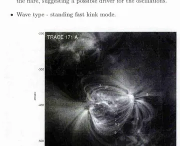
TR.ACE, with its high spatial resolution, has produced amazing images of coro­ nal loops (see Figure 1.3). Movies are produced showing actual spatial oscil­ lations of loops. The first papers detailing oscillating loops, and many other phenomena, were by Schrijver et al. (1999) and Aschwanden et al. (1999). They reported on oscillations in spatial displacements observed following a flare at 12:55 UT on July 14, 1998 (see Figure 1.6). They studied nine loops, including groups of loops. Many general properties of oscillating loops suggested by this initial study have been confirmed by further investigation:

• EUV loops - the oscillations are observed in EUV light, at a tem perature

of 2 X 10®K.

• Period length - The mean period for the loops in this study was P = 280 seconds, or around 5 minutes.

and the timing, suggested a link between the onset of the oscillations and the hare, suggesting a possible driver for the oscillations.

Wave type - standing fast kink mode.

Figure 1.6: TRACE 171 image recorded at flare initiation, 1998 July 14, 12:55:16 UT, is shown with a logarithmic grey scale. The most prominent

flare emission starts at location C\ and progresses toward position C3, straddling along the neutral line C\ — C3. The diagonal pattern across the

brightness maximum at C\ is a diffraction effect of the telescope. The analyzed loops are outlined by thin lines. Loop 4 and loops 6-9 show

pronounced oscillations. (Aschwanden et al. 1999)

The last item, the wave mode, was found by Aschwanden et al. (1999) on consideration of all of the theoretically predicted modes of oscillation as given in Edwin and Roberts (1983). For the fast kink mode, the period is given by Edwin and Roberts to be

P f a M .n k -

L

( j ° ^ ^\ )

where j is wave mode, is the phase speed, L is the loop length, po,e is the ion mass density and Bo,e is the magnetic field strength. On assuming po <C pe

of EUV loops, Aschwanden et al. found a mean period of Pfastkink = 123secs and a range of f = 0.57.8 minutes. Prom this conclusion, and on rejecting the possibilities of the fast sausage and slow modes, Aschwanden et al. concluded that the waves were fast kind modes. (See section 2.3 for a description of wave modes).

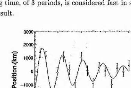
Independently, Nakariakov et al. (1999), also reported on the flare- oscillation event. They analysed a sequence of 88 images of active region

AR8270, beginning at 12:11 UT. The m ajor result from this study was the discovery of damping, shown in Figure 1.7. The damping time is found by fit­ ting an exponential, , to the oscillation curve which gives the decay time

Td. The oscillating loop was measured to have a period P — 256 seconds and a damping time Td = 870 seconds, corresponding to about 3 oscillation periods. This damping time, of 3 periods, is considered fast in solar terms and is a very interesting result.

3000p

âooq

1000

0

-1000

-2000

—3000

0 10 IS

Time (mln) 20

J

25

Figure 1.7: The tem poral evolution of the loop displacement calculated as an average coordinate of the loop position for four neighbouring perpendicular

cuts through the loop apex (diamonds), with error bars (± 0.5 pixel). The oscillation started at 13:13:51 UT on 14 July, 1998. The solid curve is the best

and gave a detailed discussion of these. The link between the flares and the oscillating loops seems to confirm the reason for excitation of the loops suggested by Aschwanden et al. (1999). However, the data is slightly biased as part of their data came from a survey of flares. Table 1.1 shows the periods and damping times found. The periods are nestled around the five minute band, so in general are longer than those observed by radio signals (where the periods are a few seconds). They found a variety of loop half-lengths, ranging from 36 — 291Mm, although the largest loop appears to be spurious for the period of oscillations corresponding to this loop is over six times larger than the average period when this loop is neglected. Accordingly, we take the range of loop half-lengths to be 36-203 Mm, giving loops of length 72-406 Mm.

Param eter Average Range Oscillation Period P 5.4 ± 2.3 min 2,3 - 10.8 min

Decay time 9.7 ± 6.4 min 3.2 - 20.8 min Number of periods 4.0 ± 1.8 - 1.3 - 8.7

Table 1.1: Properties of Coronal loop oscillations. (After Aschwanden et al. 2002)

1.5 D am ping

The reason for the strong damping is unknown although several theories have been put forward. These have been explored in some detail and a good review of possible processes involved in the damping is given in Roberts (2000).

Non-ideal effects, such as viscous and ohmic damping, optically thin ra­ diation and therm al conduction can dampen waves. However, studies of both unbounded uniform medium (e.g. Ibanez and Escalona 1993) and a slab geom­ etry (e.g. Laing and Edwin 1994) found the damping time to be at least 20 times the period, rising up to several hundred times. Thus, these effects are too small.

Wave leakage at the footpoints (De Pontieu et al. 2001) is too weak a damping force for standard chromospheric scale heights of the order A = 500km (Ofman 2002). However it could be an explanation if one takes a slightly larger scale height, say a factor of 2 bigger (Aschwanden et al. 2002).

cross-field gradients to build up, enhancing damping by viscosity or diffusivity. Resonant absorption is the process by which the global kink mode oscillation of a tube couples with Alfvénic oscillations. This means there is a transfer of energy from the global mode to small-scale oscillations resulting in a decay of the global mode. Resonant absorption has recently been reviewed by Erdélyi

(2001).

Both phase mixing and resonant absorption are discussed in a recent review by Roberts (2000) and shown to be possible. Roberts looked at the process of phase mixing of an Alfven wave. He considered an Alfven wave in an inhomogeneous plasma with Alfven speed ca{x), structured in x. This wave will propagate with transverse motions v{x,z,t)y:

V = u{t) sinkzt cos kzCA[x)t, (1.3)

where kz is the wave number and

u{t) = uq exp ~^kliy{t + ^ (c ^ )V ), (1.4)

where ?/ is the coefficient of kinematic viscosity.

Considering a uniform medium, so that = 0, a decay time Td is pro­ duced.

This produces a long decay time for a standing wave where kz — Ntt/L , where

N is the wave mode and L is the loop length. However in a magnetically structured plasma the later term in u{t) dominates giving a decay time of

Td 6

- I 1 /3

( 1.6 )

On the assumption of a spatially varying Alfven speed, on a scale of order

I — A/10, and taking a loop length of A = 10®km and an Alfven speed of

CA = 10®km s“ \ a decay time Td = 530s is obtained. This value is comparable with observed values and suggests that phase mixing or resonant absorption could be a viable reason for the strong damping of the oscillations.

phase mixing) is directly proportional to the length of the loop. There seems lit­ tle reason to accept this assumption of proportionality, unless more compelling observational support is forthcoming. The theoretically predicted damping rate in resonant absorption (see Ruderm an and Roberts 2002) is able to m atch the observational data for a reasonable range of the inhomogeneity scale I. For a tube of radius a, Ruderm an and Roberts (2002) find that I = 0.23a, which matches the Nakariakov et al. event. A more extensive study by Goossens et al.

(2002) supports this conclusion, producing a range of I = 0.15a to I = 0.5a. See also the discussion in Roberts (2002). A very recent analysis by Aschwanden

et al. (2003) offers further support for the resonant absorption idea but also points out that phase mixing remains a possibility.

1.6 SU M E R and slow waves

Recent studies by Wang et al. al (2002c; 2002a,b), a group from the Max-Planck Institute in Germany, have considered Doppler shift oscillations using data from the SUMER spectrometer on SOHO. They found evidence of oscillations in hot active region loops which are markedly different from those observed by TRACE. Indeed, there is no sign of these oscillations in the TRACE lines of 2 X 10®K; the oscillations are observed only in hot plasma greater than 6 x 10®K.

• The oscillations coincide with loops seen in hot soft X-ray, not. EUV, loops.

• Period - the SUMER oscillations have distinctly longer periods {P =

17min) than the TRACE transverse oscillations, although they have a similar decay rate.

• The excitation of the oscillations is unclear as, unlike TRACE data, few events are associated with flares.

• Wave type - slow mode.

The definition of the waves as a slow mode was confirmed by Ofman and Wang (2002). They used a 1-D MHD code to model the hot loops and concluded that the waves are slow mode magnetoacoustic standing waves.

Param eter Average Range Oscillation Period P 17.6 ± 5.4 min 7.1 - 31.1 min

Decay time 14.6 ± 7.0 min 5.7 - 36.8 min Number of periods 2.3 ± 0.7 1.5 - 5

Table 1.2: Properties of hot soft X-ray loop oscillations. (Wang et al. 2003)

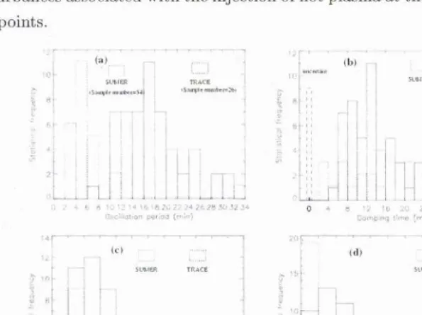
al. (2003) conclude that the excitation of these oscillations may be pressure disturbances associated with the injection of hot plasma at the oscillating loop’s footpoints.

(a)

n

. J u

jtj

!

c 10 ! 2 • 16 : b 20 22 26 5C> J 2 J CsciMoiton period (ru n )

nd,„..hJ J

2 0 AO 60 80 100 120 U O 160 180 2 0 0 2 2 0 7 40 Oopplcf s n J t arnp'itudO ( n r r /s )

(I»

RIMER TRACE

0 4 b 12 I t 2b 24 28 S .' i t

Oom p.ng dm e (m in)

ii\}

SLMER TRACE

8 12 "6 20 24 / b 32 36 4 0 44 Oisploccm cr* am plitude (Mm)

Figure 1.8: Distribution of the physical parameters of the 54 SUMER Doppler-shift oscillations (solid histograms), and distribution of the param eters of the 26 TRACE loop oscillations (dotted histograms) obtained by Aschwanden et al. (2002). a) Oscillation periods, b) Damping time. The

number of TRACE loop oscillations whose damping time could not be evaluated is represented with a dashed strip, c) Measured maximum Doppler

velocity amplitude for SUMER oscillations and the maximum transverse speed for TRACE oscillations, d) Derived displacement am plitude for SUMER oscillations, and the transverse motion amplitude for TRACE

Chapter 2

M HD waves

Before a discussion on magnetohydrodynamic (MHD) waves in the solar atmo­ sphere, it is necessary to consider some of the basic wave forms, their properties and how they relate to each other.

2.1

M H D equations

The solar atmosphere is a stratified and strongly structured magnetic medium. We use the equations of MHD to describe the wave motions that may occur. Taking velocity v, magnetic field B, pressure p, density p, gravity g, magnetic permeability p, and adiabatic index 7, we have:

• Equation of continuity

^ -I- div(pv) = 0. (2.1)

• Equation of motion

p ( ± + (v-Vv)) = - V p + i ( V X B) x B + p g . (2.2)

• Induction equation

— curl ( v X B ) , (2.3)

for an electrically ideal fluid.

• The solenoidal constraint from Maxwell’s equations,

• Energy equation

| + v . V p = ^ ( | + v . V p ) , (2.5)

for an adiabatic medium. • Perfect Gas L^w

P = ’^ p T , (2.6)

where k s is the Boltzmann constant, m is the mean particle mass and T is the tem perature.

2.2 Sound waves

In the absence of a magnetic field (B = 0) and gravity {g = 0) we obtain the hydrodynamic equations with which we can investigate sound waves. Consider a compressible fluid at rest with undisturbed uniform pressure po and density Po- Suppose that as a result of a small disturbance the pressure and density are changed so that

P = P o+ Pi, p = Po + Pi,

where pi < po and p\

po-Linearising the equation of continuity (2.1) and the equation of motion (2.2) respectively, by neglecting squares of small quantities, we obtain

4- podiv v '= 0, (2.7)

d'v

^^~dt ~ (2.8)

Linearising the energy equation (2.5) and the perfect gas law (2.6) gives

^ + v . V p „ = ^ ( ^ + v . V p o ) , (2.9)

Pi — ^ {pi'^0 + PqTi) , (2.10)

with the equilibrium state

We introduce the sound speed Cg,

1/2

Cs _{po )} (2.12)

Eliminating the pressure terms p\ and pq from equation (2,8) using equa­

tions (2.9) and (2.11) and using the vector identity

curl curl v = grad div v — V^v,

shows that v satisfies the 3-D wave equation,

(2.13)

Thus, the solution of the hydrodynamic equations is a sound wave w ith speed

C s .

W ithout loss of generality, consider the æ-component of velocity Vx- The general solution of (2.13) for Vx is

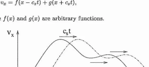
% = f{ x - Cst) + g{x + Cgt),

where f{x) and g{x) are arbitrary functions.

(2.14)

Figure 2.1: A wave of arbitrary shape travelling at speed Cg in the æ-direction. Consider Vx = f {x — ct). In any plane x ^constant, the velocity changes in time. However there exist co-ordinates x and t such that x — Csi—constant,

X —constant-t-Cg/ when Vx will have the same profile. This is illustrated in

Figure 2.1. A wave such as this which propagates at a certain speed is called a travelling wave. The opposite of a travelling wave is a standing wave, where the wave oscillates but does not propagate. A sound wave is also a longitudinal

particles. A wave where the particles oscillate in a direction perpendicular to the direction of the wave is called a transverse wave.

2.3 M agnetic waves

The presence of a magnetic field changes the situation. In an infinitely con­ ducting fluid, the fluid particles are ‘tied’ to the magnetic lines of force. So any attem pt to initiate a sound wave will result in variations in the magnetic field. In 1942 Hannes Alfven pointed out that, by analogy with the transverse vibrations of stretched strings, these variations will cause local compressions and rarefactions of the lines of force, ie the lines of force may oscillate (Alfven 1942). This is the simplest type of MHD wave, the so-called Alfvén wave.

Mathematically we need to consider the linearised forms of the equation of motion (2.2) and the induction equation (2.3). Write B = Bq + b, where Bq = (0,0, Bo) is the uniform background magnetic field and b is the perturbation

where |b| is small. Recall the vector identity,

(a • V )a = V ^ j - a x curia. or

(B . V )B = V Q jB A + curlB x B,

where B = |B| = Bq + 2B ■ b. Using this vector identity, the equation of motion (2.2) with g = 0 reduces to

We restrict attention here to motions that are incompressible, so that divv = 0. Then considering the divergence of this equation and recalling that div B = 0, we find that

,2 /

^ 7 +

Linearising the induction equation (2.3) using the vector identity

curl(a X b) = adiv b — bdiv a + (b • V )a — (a • V )b,

gives

Simply differentiating one of the equations (2.17) and (2.18) with respect to z and the other with respect to t shows that both b and v satisfy the wave equation

^ ( v , b ) = 4 ^ ( v , b ) , (2,19)

where ca is the Alfvén speed given by

n2

ca = — (2.2 0)

POf^Q

There are also motions with div v non-zero; these are the magnetoacoustic ’modes, found by considering how all the linearised equations interact. Taking

P = Po +Pi i P = Po + Pis B = Bo + b, as before, the linearised MHD equations are:

^ + (v-V)po + Po(V-v) = 0, (2.21)

S'Y 1

P O - ^ = -V p i + - (V X b) X Bo, (2.22)

^ = V X (v X B o ) , (2.23)

^ + v V p o = c ? ( | ^ + v V p o ) . (2.24)

Differentiating (2.2 2) with respect to t and substituting for ^ from (2.24)

and for from (2.23) gives:

p o ^ = C?V(V ■ v) + V X (V X (v X Bo)) x (2.25)

We consider a Fourier component

where k = {kx^ky,kz) is the wavenumber vector of magnitude |k| = & =

ky + Let the direction of propagation vector k be at an angle 6 to the equilibrium magnetic field Bq. Then equation (2.25) gives the dispersion

relation

- {c\ + cj)w^A;^ + cos^ 6> = 0, (2.26)

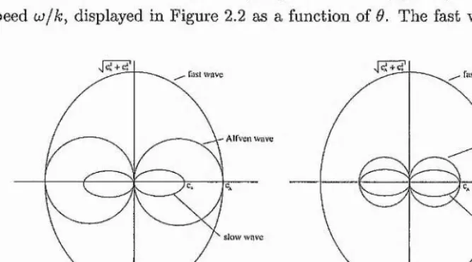
where 6 is the angle between k and Bq; dispersion relation 2.26 has two real roots for (four roots for oj). In general, including the Alfvén wave there are three distinct waves: the Alfvén wave is one,' and the other two are magne­ toacoustic waves which are called the fast and slow waves. The relative wave speeds of the solutions of equation (2.26) can be seen by polai’ plots of the phase speed w/&, displayed in Figure 2,2 as a function of 9. The fast wave speed c/

fast wave fasl wave

Alfven wave Atfvcn wave

slow wave slow wave

(a) CA > Cs (b ) CA < Cs

Figure 2.2: Polar plots of the three MHD wave speeds.

is both super-sonic and super-Alfvénic and is associated with the speed Cfast

which can be w ritten in terms of Cg and ca through (Roberts 1991)

^fast T (2.27)

The slow wave speed is both sub-sonic and sub-Alfvénic and is associated with the speed (or ct) which can be w ritten in terms of Cg and ca through

(Roberts 1991)

1

This speed generally arises in the modelling of waves in a flux tube and so is commonly called the tube speed.

Another property of waves to consider is the shape of the waves. For waves propagating in non-uniform media, say in a flux-tube or across an interface, either surface or body waves can arise (see Figure 2.3). The surface wave is located predominant at boundaries, whilst body waves exist throughout.

(a) Surface wave (b) Body wave

Figure 2.3: Waves profiles across a flux tube or slab (After Roberts 1981a,b; Edwin and Roberts 1983)

Also, for a magnetic slab or tube these modes may be geometrically clas­ sified as sausage or kink modes (see Figure 2.4).

(a) Sausage mode (b) Kink mode

Figure 2.4: Modes of oscillation of a magnetic flux tube

(or travelling) waves in which the energy is transferred by means of vibrations, like waves on a string.

2.4 W aves in a structured m edium

Consider a basic state in which there is a magnetic field of strength aligned with the z-axis in a Cartesian co-ordinate system. Let po, Vo and Bq all vary in a direction perpendicular to the applied magnetic field. W ith an equilibrium condition of pressure balance, we have a basic plasma state of the form

d ( B ^ \

Po = Pq{x), Pq - po{x), — f po + “ ) = 0. (2.29)

Suppose that as a result of a small disturbance the pressure, density and mag­ netic field are changed so that p = Po + Pi, p — Po+Pi > B = B o + b , where

Pi Po, Pi -C Po, |Bo| |b|. Linearising the equations of continuity, motion, induction and energy equations (2.1)-(2.5), with p = 0, results in

^ + div(pov) = 0,

P^~ô7_ut “ (p^ "i— Bo • b j -I— (Bo • V )b H— (b • V)Bq,_{p J p p} ^ = curl(v X Bo), V • b = 0,

~ -}- V • Vpo = cl -f V • Vpo^ , (2.30)

where Cg = {'ypoix) jpq{x))^1'^ is the local sound speed (a function of x). Using

the variables

V = d iv v , r = PT = P + -B o • b, (2.31)

ox p

the linearised equations (2.30) yield three partial differential equations (see, for example, Roberts 1981a)

Po dx + 4 ) ^ - Poc^r) , (2.32a)

Po ^2/ = ^ (po (cg + c3i) A - poc^r), (2.32b)

differ-ential equation by taking Fourier components. Writing

'Ox ~ Vxix) exp i(tvt + kyy + kzz),

the governing differential equation is (Roberts 1981a)

= po(x)(klcl^(x) - w^)%, (2.33)

d ( PQ{x){klc\{x) - W^) dv^ \ _ , w, 2^2 / \ , ,2,

dx \ rin?{x) + k"^ dx

where

2 _ {hlcl{x) uj‘^){klc\{x)

-(cg(:r) + c2(:z;))(A:2c2(a;)-w2)'

the quantity introduced in the above, may be positive or negative.

Solutions of this equation are not straightforward. In particular, there exists continuous spectra of solutions connected with the singularities at uP" =

kl(P^{x) and up = kl(^{x). Two special cases most frequently analysed are the magnetic interface and the magnetic flux tube. However, the simplest case to consider first is when po, ca and Cg are all constants, corresponding to a uniform

unbounded atmosphere.

2.5 W aves in a uniform m edium

For a uniform medium, equation (2.33) reduces to

{k^pA ~ oP) ^ — 0- (2.35)

This equation yields the Alfvén wave, uP — with the form of Vx{x) arbi­ trary (and determined by initial conditions). On taking a Fourier component

Vx oc exp{ikxx), the differential operator in equation (2.35) yields the magne­ toacoustic waves,

rrP + k l + /Sy = 0; (2.36)

that is

+ P k l c l c \ - uj‘^P {cl + c'a) = 0,

where = k^. + k^ + k^.

this implies uP/k^ lies between Cy and the smaller of Cg and corresponding to a slow wave, or above the larger of Cg and c^, corresponding to the fast wave.

2.6 W aves at a m agnetic interface

B q P o _{B e P e}

x=0

Figure 2.5: A magnetic interface æ=0 separating a plasma with density po and field strength Bq in æ < 0 from a plasma with density pe and field strength Bg

in rr > 0.

A medium with an interface across which the physical properties change sharply can support surface waves. Consider an interface where the magnetic field changes discontinuously from a constant Bq to a constant Bg, so that

Ba(x) = ^ (2.37)

I^Bg, x > 0, as shown in Figure 2.5.

For a uniform medium, and ignoring Alfvén waves by setting Vy ~ Çi and

ky = 0, equation (2.33) reduces (in æ < 0) to

^ - VP?V^ = 0, (2.38)

where

here Cgo is the sound speed and cao is the Alfvén speed in x < 0. In the region æ > 0, = TTie and generally the ‘0’ subscripts are replaced by ‘e’ subscripts. Thus the differential equation (2.38) has a simple exponential solution,

%=(%) = = < O' (2.40)

Assuming that Vx{x) —>■ 0 as |æ| —> oo requires that mo, mg > 0. A condition of continuous velocity at a; = 0 is satisfied by taking ao = ae.

A second boundary condition is that of continuous total pressure at the interface. To apply this, we need an equation relating Vx and p r, namely

rrir dx (2.41)

with a similar expression applying for a: > 0 with ‘e ’subscripts. Using (2.41) yields the dispersion relation (Roberts 1981a)

Poikl^AQ - w'^)me + pe{PzPle ~2^2 = 0. (2.42)

This is the dispersion relation governing magnetoacoustic surface waves on a single interface. Rewriting (2.42),

'AO W'■Al

'Ae

-mope

mePo (2.43)

implies the left-hand side of the fraction mush be negative, since mo, mg > 0. For this to be true w/A^ must lie between the Alfvén speeds of the two media. It is found that in general there are two surface waves, the slow and fast waves (Roberts 1981a).

2.7 W aves in a m agnetic slab

Flux tubes are an im portant consideration for the solar atmosphere. A first approximation to a flux tube is a magnetic slab, which is mathematically easier to discuss than the cylindrical geometry of a flux tube. The magnetic flux tube is discussed separately (see Section 2.8).

k

Be Pc Pc

Bo

Po Po Pe Pc

Be

-Xo Xo

Mathematically, the description of the equilibrium state is:

PoM,Po(a;),Bo(a;) = I i < o, (2.44) [pe,Pe,Bg, |rc| > æo.

The magnetic slab is very similar to the magnetic interface, but with two boundaries at which the physical properties change sharply. Mathematically, the only difference is the equilibrium state, which is more bounded. Conse­ quently the flow i)x is described by the solution of the differential equation (2.38) with 0 as |a:| oo:

%(a;) = <

Q,^gme(a: æ < —Xq,

CKO cosh mox -f /3q sinh mox, |z| < zo, (2.45) z > æo,

where cxg, qq, /^e, &re constants and mo,e are given as in Equation (2.39). It is necessary that mg > 0 (to satisfy Vx —> 0 as |rc| —> oo), but ttIq may be positive or negative (so mo may be positive or imaginary).

To consider odd solutions take ao = 0, and for even solutions take /?o — 0. Applying continuous boundary conditions at æ = ±a;o for velocity and pressure, as in the case of the single interface, gives a series of relationships for the constants in equation (2.45). Ensuring a non-trivial solution determines the dispersion relation (Edwin and Roberts 1982),

Pe{klc\^ - w^) TTto^o + PoiklcAo ~ w^)mg = 0, (2.46)

where ‘tan h ’ corresponds to the odd solution and so is called the sausage mode, and ‘coth’ corresponds to the even solution and so is called the kink mode. As noted earlier, mg is taken to be positive, whereas m^ may be positive or negative.

For the special case of an incompressible fluid, mo and mg tend to giving

.2 , _ 2 } tan h l coth J Pocjio + PeCjie { } k^XQ

(2.47)

k'û f tan h l

Relating the magnetic slab to a flux tube, so that it resembles a coronal loop, consider a slender slab. Slender implies looking at the propagation of waves whose wavelength in much greater than the width of the slab, i.e. kzXQ >C 1. So taking tanhAî^a^o ^ kzXQ and cothA-^xo 1/kzXQ^ equation (2.47) reduces to

UJ klc\Q{l 4- P e /m ( 4 e /4 o " l)^za;o), for the sausage mode,

k lc \^{l + po/pe(c^o/c^g - l)A:^æo)j for the kink mode. (2.48) These results are displayed in a dispersion diagram (see Figure 2.7), which also shows the behaviour for general kzXQ,

3

2

<

1

oL

0.0 0.5 1.0 1.5 2.0

kxQ

Figure 2.7: The phase speed ukz as of a function of kzXQ for magnetic surface waves in an incompressible medium with c^o < c/ie- A full curve represents

the sausage mode and a dashed curve the kink mode. (Note: k = kz.)

For a more complete description of the solutions of Equation (2.46), see Edwin and Roberts (1982, 1983).

2.8 W aves in a m agnetic flux tu b e

A better model of a flux tube can be obtained by using a cylindrical system instead of cartesian co-ordinates. The equilibrium setup is the same as for a magnetic slab except that the interface is r = a instead of x — ±a:o- Analogous equations to Equations (2.32) are found which can be reduced to an ordinary differential equation by taking Fourier components. Writing

the governing differential equation for R{r) is

d?R 1 dR

d>p2 dr rriQ -f- ^ ) iî = 0. (2.50)

This is a Bessel equation. Taking a bounded solution at r = 0 and no radial propagation of energy in r > a, there is a simple Bessel solution,

R{r) = {

In{mor), m l > 0

^ 0 S r < a

Jn{nor), nl = -m § > 0 (2.51)

A i Knimev), r > a,

where v4o and A \ are constants and 7^,, and Kn are Bessel functions of order n (Abramowitz and Stegun 1964). As with the magnetic slab, taking continuous velocity and pressure at the interface r = a yields a dispersion relation.

sausage

waves

10 20 30 40 ka

Figure 2.8: The phase-speeds u /k z of body modes under coronal conditions

{cAe^CA > Cge, Cgo), according to Edwin and Roberts (1983). (Note: k =

VAe = C /le , = C /l-)

Considering < 0, the dispersion relation is (Edwin and Roberts 1983)

, 2 \ „ _{+ po{k^c\,}

-Kn{mea) 0. (2.52)

Figure 2.8 illustrates the behaviour of waves under coronal conditions, i.e. when caciCao > Cae, CgQ. Edwin and Roberts discovered that in such cir­

2.9 G ravity

The model we investigate looks at two new effects, one of which is the influence of gravity. It is a basic problem to consider the acoustic equations (i.e. the MHD equations with B = 0) and including the stratification effect of uniform gravity g = (0,0,g). The effect of gravity seriously complicates any discussion of magnetohydrodynamics. Here, we take a first step in this investigation by considering what happens to acoustic waves in the absence of a magnetic field. We may expect that in the presence of a magnetic field, slow waves will behave rather similarly to sound waves.

In the absence of a magnetic field, but with gravity present, the governing system of equations is now

^ + div(pv) = 0, (2.53)

P T (v • V v)^ = - Vp + pg, (2.54)

2

(

— + V . Vp = Cg + V • V pJ , (2.55)

p = ^ p T . (2.56)

To examine the equilibrium state of this system, consider w hat happens when V = 0 and = 0. The momentum equation (2.54) reduces to

—Vpo + Po p — 0,

that is,

^ = pop- (2.57)

The z-axis has been aligned with the direction of gravity, pointing downwards. The perfect gas law (2.56) provides a relationship between po and po,

Po === — Poffb- _m (2.58) We consider Tq to be a function of 2: only, i.e. Tq = T q [ z ) for some arbitrary

sub-stitiiting P q { z ) — into equation (2.57) we obtain

dpo mg

Po,

- d p o = - ^ d z . (2.59) Po KgTo

Thus

Po = Po(0) = exp . (2.60)

Introducing Aq, the equilibrium pressure scale height, defined by

Ao(.) = M M d = f l , (2.61)

mg POP

gives

Po(^) =Po(0) expn(z), n { z )= ir-r^ - (2.62)

Jq Ao(2:j

Equation (2.62) gives the distribution of equilibrium pressure po(^) in terms of the pressure po(0) at the arbitrary reference point % = 0 and the pressure scale height Ao(z).

Linearising the system by taking

P = Po(^) + p i(a;,z,^), P = Po(4 + Pi(a:,z,^),

where pi <C po, Pi < Po, and taking

V = (væ, 0,112),

we produce the following set of linearised hydrodynamic equations:

+ Po^ + VzPq = 0, (2,63)

P O ^ =_{dt dx ’} (2.64)

dpi

dt + gpoVz — Cg + ii%pA . (2.66)

Differentiating equation (2.65) with respect to t gives

We can substitute for ^ from equation (2.63) to obtain

We can then substitute ^ in terms of po and Vz only, by considering equation

(2.66):

V j ~ 9 PoVz

= (-P 0 V - Dzpo) + C^HzPo - p Po llz

= -CgpoV - gpoVz^ (2.68)

Substituting this result into equation (2.67) reduces the equation to one con­ taining only the variables po and Vz and their derivatives:

d ‘^Vz <9 r 2 A 1 A /

l-CgPoA - ppo iizj - PPoA - puzPo

= C g P o ^ + A [cIp'q -h po(C g)'] -I- p p o ^ + g vzP o - ppo A - gvzp'o

2 ^A .

<?sp'a + P o { l9 — ^

Po

<9nz

.

On writing A = we have reduced the hydrodynamic equations to a single second order partial differential equation for Vz-,

Following Rae and Roberts (1982), we write

- 1/2

Q = py^CgVz, or Vz = Q —---■ (2.70)

Cg

The new differential components are:

and

dvz _{P ô '/'} Q

Cs dz dz

1/2

_

<

, -1/2

P ô '/'

^ H - O d Cg oz dz

1

■

P ô '/' a q Cg dz

P ô '/' a q

■

0 _ 7P0

Po

1^ 1 1

- oQt--- ÔT7T— POP,

_-3/2_/

dz 2 (7Po)^/^Po

9 ^ ^2 '

Po = Pop,

PO CgPO

7

In a similar fashion, we may obtain an expression for the second derivative of

Vz with respect to z.

d‘^1 _Po1/2

dz^ dz'^ P ô '/'Cs cj dz19 dQ 3 Po 4 Cg \Cg / / 7 P V ^ l Po^^^7 P P o ^2 Cg Po Substituting these expressions into the second order partial differential equation (2.69) leads to an ordinary differential equation in Q, The coefficient of is

- 1/2

Po _{7P + 7PPo}- 1/2 _{= 0.}

The coefficient of Q is given by

3 Po 7^P^ _{IP o ^ ^ ^ P P o + 7P -lPo^^^7P} 4 Cg c^ 2 Cg c^ Po 2 Cg cg

Cg _4 cg37P = _Cg '1 TP _{_4 cg}

_

Cg [2 _^g

2po

2^ ' ,2\/>

4 cl

2^21

(cg)^ = 7P - c:2 A

Thus, overall our equation for Q is

§ - ? g + n^e = o. (2.71)

where

(2.V2)

Chapter 3

Coronal loop oscillation m odel

3.1 Coronal Loop m odel

W ith this model of a coronal loop we investigate the importance of two effects: gravity, and the addition of a chromospheric layer below the corona. Consider a coronal loop of half-length L with its footpoints of extent h embedded in the chromosphere (see Figure 3.1).

Corona

h \ \ Chromosphere

Figure 3.1: Coronal loop of half-length L with chromospheric footpoints of extent h.

Assuming the loop is symmetric about its apex means that only half the loop need be considered. It also simplifies the geometry of the situation so that a cartesian co-ordinate system may be used instead of a cylindrical system. The half loop is straightened out with the %-axis taken along the loop. The apex of the loop is taken to be at ^ = 0 (see Figure 3.2).

To investigate oscillations in such a loop, we consider sound waves propa­ gating vertically in a stratified atmosphere where magnetic effects are ignored. The stratification comes from the consideration of uniform gravity g = (0,0, p), aligned with the z-axis. To investigate the role of the two layers, corona and chromosphere, the sound speed is taken to be a function of z. This function,

Top of Loop

Base of Loop

Figure 3.2: Symmetrical coronal loop model aligned with the z-axis, with apex at z = 0. Gravity is aligned with the z-axis.

first is a step function

Cg ; Z ^

L z <i L -\- h.) (3.1)

where Cc denotes the sound speed in the corona and Cp is the value of the sound speed in the chromosphere/photosphere. The second case considers a continuous variation in sound speed,

Cs(z) = co(l - (3.2)

the sound speed decreases (at a steady rate determined by a) from a value cq at z = 0 down through the corona and into the chromosphere.

This setup leads us to consider the linearised hydrodynamic model. As detailed in section 2.9, this model leads to the Klein-Gordon equation for Q,

namely.

dt^ — c„

where

Here a dash ' denotes differentiation with respect to z.

(3.3)

(3,4)

We note that in the special case of zero gravity, we recover pure sound waves (section 2.2); with = 0, the Klein-Gordon equation (3.4) reduces to

which is the one dimensional wave equation with propagation speed Cg.

Returning to the Klein-Gordon equation (3.4), with Q. ^ 0 and taking a Fourier component in i, Q oc where u is the wave frequency, we find that (3.4) reduces to the ordinary differential equation,

, 7.2

dz^

where

-{-A;4z)Q = 0, (3.7)

L < z < L + h.

3.2 Case 1 - Isotherm al atm osphere

Taking the step function form of the sound speed (equation (3.1)) is equiva­ lent to considering the corona and chromosphere each as distinct isothermal atmospheres. Under isothermal conditions the sound speed is constant and reduces to

« ' = i

Thus we obtain the cut-off frequency Q = 'yg/2cs first considered by Lamb (1909, 1932).

3 .2 .1 D isp e r sio n r e la tio n

In these circumstances a trigonometrical solution of the ordinary differential equation (3.7) exists, namely

A i cos kcZ -h B \ sin 0 < z < L,

Q ~ ^ (3.10)

A2 cos kpZ + B2 sin kpZ, L < z < L + h,

where A i, A2, Bi and B2 are constants and k^p are given by equation (3.8).

Since there are four constants (Ai, A2, B i and B2), four boundary con­

at the loop footpoint z ~ L h.

The condition = 0 at the loop apex is chosen for convenience; we are assuming that the oscillations have a node at the summit of the loop. Alterna­ tively, we may consider that = 0 at the loop summit. The condition = 0

dJi z ~ L -\-h means that there is no vertical motion at the loop footpoint; this condition is chosen to reflect the line-tying effect of the dense chromosphere on any motions generated within the corona. The equilibrium density po(z) varies exponentially but since Q = py^CgVzi the requirement that Vz = 0 at z = 0 and

z = L h means that

Q = 0 at z = 0 and z = L + h, (3.11)

The model must be consistent across the boundary between the corona and the chromospheric base. The velocity, must be continuous at the inter­ face z = L, In view of the relation Cg = 7Po/ Po (equation 2.12), giving

and the fact th at the equilibrium pressure o î p q{z) is continuous, continuity of

Vz implies

Q is continuous across z — L. (3.12)

Our fourth boundary condition is found by considering the integration of the differential equation (3.7) over a small neighbourhood oî z = L. The details of this calculation are given in Appendix A, and lead to the condition that

~ - is continuous across z = L\ (3.13)

dz 2Aq

here Ao (z) is the pressure scale height related to the sound speed by

Cg = ?gAo. (3.14)

The boundary conditions (3.11) at z = 0 and z = L + h reduce Q to

0 < z < L , (3,15)

Ki z = L, the two boundary conditions (3.12) and (3.13) give:

B \ sinkcL = Bg sin (—/%),

1 1

k^Bi cos kcL — —-T—B \ sinkcL — kpB2 cos kp{^—/i) — —-r—Bg sin (—/i).

2tIxQ 2A.p

The condition for a non-zero solution of these two equations for B \ and Bg is th at the determ inant of the coefficients must be zero:

s'm kr.L

kr cos krL _2Ac

sin kph

sin kr.L —kpcos k j i —_P'" ôx- sin _{2 A.} knh = 0. (3.16)

Expansion of the determ inant (3.16) results in the required dispersion relation for a two-layer system stratified by gravity,

2^ r ) sin/cph, - kp sin kcL cos kp h

-— kcSinkphcoskcL = 0. (3.17)

The wavenumbers kc and kp are defined in equation (3.8).

3 .2 .2 A n iso la te d m ed iu m

To understand the dispersion relation (3.17), we can check that when taking the limits h —)• 0 or B —)• 0 the expected result is obtained. The expected result is found by considering a solution of the ordinary differential equation (3.7) in an infinitely wide, isolated slab of height L when k is constant, so that the chromospheric layer is ignored (see Figure 3.3).

Figure 3.3: A coronal region of extent B, bounded at z = 0 and z = L.

Again the differential equation (3.7) has a trigonometrical solution, namely,

Q = Acos kcZ -\- Bsin kcZ^

used. Thus imposing Vz — Q = 0 a t z = 0 reduces Q to

Q = B sin kcZ.

Imposing Q = 0 at z = L gives

sin = 0. (3.18)

Thus,

kc = — , n = 1,2,3,... (3.19)

Expanding kc in terms of w, using the coronal part of equation (3.8), gives

+ (3.20)

Now consider the full dispersion relation (3.17) under the limit —> 0, implying that sin kph -> 0 and cos kph -> 1. The reduced dispersion relation is

sinA:cB = 0. (3.21)

Thus we recover kcL — mr,

A similar solution is found when considering propagation of sound waves in a purely chromospheric layer, obtained by taking the limit B —> 0. In this case the dispersion relation (3.17) reduces to

sin kph — 0. • (3.22)

Thus kph = tttt; using the chromospheric part of equation (3.8) leads to the result

^

3 .2 .3 S h a llo w ch ro m o sp h eric layer

dispersion relation may be expanded:

s'm kph « kph [l - Oikph"^)] ,

cos kph % 1 - 0{kph?‘).

Using these expressions, the general dispersion relation (3.17) reduces to

— I —— — ——j kph sink^L — kpsink^L —■ kph k^ cos k^L — 0. (3.24) 2 \ Ac Ap J

dispersion relation can be rewritten in the form This reduced

sin kcL = ef {kcL) (3.25)

where e = kph <C 1. To achieve this we divide equation (3.24) by kp. It is useful to restrict the occurrences of kc to the combination /zgB, so we also multiply the equation by L. Thus,

” ( -J— ~ j sin _{2 \ Ac Ap /} kcL — kcL cos kcL , _J (3.26)

sinkcL — ^ kph

so that

1 / 1 1

\

sin kcL — -—- kcL cos kcL.

kpL (3.27)

Since e is small, we consider the limit e —)• 0. This reduces the situation to simply sinArcB = 0, or kcL = mv, with n = 1,2,.... Since we are looking at

sin kcL = ef{kcL), where e is small, we may write

kcL — Th'K ”{~ £ Cfi^ (3.28)

for some constants

Cn-By calculating sin(n7r + eC^) and cos(n7r + e(7n), an expression for f{kcL) in terms of Cn can be found:

sin(n7r + eCn) = sinnTr cos eCn + cos mr sineCn

= 0 X coseCn + (-1)"«C „(1 - 0(t'^CD)

« {—l)^eCn

cos(n7T + e C n ) — cosnTT coseCn — sin n-TT coseCn

= ( - l ) ’^(l - O(e^C^) - O x coscCn

pe (-1 )" .

(3.29)

Substituting (3.29) and (3.30) into f{kcL) (equation 3.27) gives

f{nir + = (3.31)

By substituting this expression for f{kcL) into equation (3.26) we obtain Cn,

sin(n7r + e C n ) = e /( n 7 T + e C n ) ,

1 / 1 1

(-l)"€C n = e _{2kp y Ag Ay}

n7re(“ l)"'

k p L

( —1 )”' € Cn

kpL (n7T + e C n ) ( - l ) ’

to first order. Hence, n7T

C n — (3.32)

We now have a solution, kcL, of the dispersion relation for wave propagation in the limiting case kph <C 1, namely

k c L = 717T + eCn,

, , h

= n7T I 1 — — (3.33)

Since k^ — (w^ - Og)/cg, this leads to the solution

^ ( W ) " = (3.34)

that is,

L2 (3.35)

3 .2 .4 D im e n s io n le s s d is p e r s io n r e la tio n

For numerical treatm ent of the full dispersion relation we write it in dimension- less form. This is easily achieved by multiplying the equation by Ac:

1 — ^ j sin kcL sin kph — kpAc sin kcL cos

kph->/

— kcAc sin kph cos kcL — 0. (3.36)

2 V Ap

The wave frequency u enters through the wavenumbers kc and kp defined in equation (3.8). We rewrite the dispersion relation so that w is more explicit. Set

to — — , (3.37)

a dimensionless measure of the frequency w. It is convenient to express kp Ac, kcAc, kcL and kph in terms of w and the param eters

As shown in Appendix B, the dimensionless dispersion relation describing wave propagation in a two-layer system stratified by gravity is

1 \ 1/2 / a2 / 1 \ \ 1/2

(1 - r) sin ( -J- (ü7^ - l) j sin ( — (

1/2 /g2 \ 1/2 ^ l \ \ l/2

I — W I I sin 1 (cj^ — l) I cos I ( w'"

2 V 4 J \ 4 r \ r

(

% ( w ' - l ) )

\ 4 r \ r / / \ 4 / \ 4 r \ r

1/2 / /2 / l \ \ l / 2 / ,2 \ l /2

(3.39) The three new param eters r, s, and / have meaning in term s of the model. The constant r shows the relation between the corona and the chromospheric layer, using as a measure the relative squared sound speeds, and Cp (or, equivalently, the pressure scale heights Ag and Ap). The param eter ( is a measure of the chromospheric extent. Finally, s is a measure of the length of the loop and consequently varies from loop to loop.

sound speeds (see Appendix C for the details) obtaining

Ac % 5 X lO'^ km, Ap « 500 km (3.40)

and

c,c ~ 152 km s , Cp « 15 km s . (3.41)

Using these values we can calculate a value for the fraction r,

Ap 1.4 X lO^m 1 y ^ ’ ■ = Â ; = 5 X W m “

3ÔÔ-The extent of the chromosphere is very small compared to the radius of the Sun, but the actual value is unclear. Values ranging from 1000 km [2] to 2500 km (Lang 2001), or even up to 10000 km (Golub and Pasachoff 2001) are suggested. However, since the pressure scale height in the corona is of the order 10‘^km, this tells us that generally /3 <C 1.

The average loop length observed by TRACE in the corona is 110 Mm (Aschwanden et ai 2002). This gives an average value of s of about 10. In general we consider short loops to have s <C 1 and long loops to have s %$> 1. We can use this definition of ‘short’ and ‘long’ to analyse further the dispersion relation for wave propagation in an isolated coronal atmosphere (section 3.2.2). We found the dispersion relation to be

.2^2

that is.

In terms of the dimensionless variables w and s,

4n^

= 1 + (3.43)

For a short (s 0) loop, oo; for a long (a — oo ) loop, —> 1, i.e.

w % flc‘ (3.44)

L (see Figure 3.5). The period r of an oscillation lies below 27t/Üc

Figure 3.4: Sketch of the dimensionless wave frequency w(= oj/Q.c) against

s — L /k c for an isolated coronal structure, showing a cut-off frequency

Qc-T/K

2n

I

Figure 3.5: Sketch of the period r{— 2?r/w) against dimensionless loop length

27r/ric-3.3 Case 2 - C ontinuous sound speed

We return to the Klein-Gordon Equation

where

In section 3.2 we took the sound speed to be a step function w ith Cg taking different constant values in the coronal and chromospheric layers. Here we consider the continuous function

Cs = co(l - z > 0, (3.45)

where a (&0) is a constant so that the sound speed squared decreases from a value = Cq at the loop apex {z — 0), through the corona and into the chromospheric layer, at a constant rate a. W ith this form of the sound speed,

becomes

Taking a Fourier component in t, so that Q oc exp icjt, reduces the Klein-Gordon equation from a partial differential equation to an ordinary differential equation, namely

+ (3.47)

dz"^

V c2(z)

The presence of the combination (1 — az), in both P^(z) and c^(z), suggests a suitable change of variable. We write

u = 1 ~ az. (3.48)

In order to make this change of variable we need to find the differential opera­ tors:

d \ 2

d d d

dz du

d? d d (