Effective design and simulation of surface based lattice structures featuring volume fraction and cell type grading

(1)

Contents lists available atScienceDirect

Materials and Design

j o u r n a l h o m e p a g e : w w w . e l s e v i e r . c o m / l o c a t e / m a t d e s

Effective design and simulation of surface-based lattice structures

featuring volume fraction and cell type grading

I. Maskery

a,

_*

_{, A.O. Aremu}

a

_{, L. Parry}

b

_{, R.D. Wildman}

a

_{, C.J. Tuck}

a

_{, I.A. Ashcroft}

a a_{Centre for Additive Manufacturing, Faculty of Engineering, University of Nottingham, Nottingham NG8 1BB, UK}

b_{Added Scientiﬁc Ltd., Nottingham Science Park, Nottingham NG7 2RH, UK}

H I G H L I G H T S

• Surface-based lattice structures were designed and examined with ﬁnite element analysis to determine their elastic moduli.

• The moduli were found along three loading directions for each lattice, and these were correlated with their volume fractions.

• A factor of three difference was found between the moduli of the least stiff and most stiff lattice types.

• The determined modulus-volume

fraction relationships accurately predict the moduli of graded lattice structures.

• We demonstrate a design approach for hybrid lattices which identiﬁes and corrects regions of low structural connectivity.

G R A P H I C A L A B S T R A C T

A R T I C L E I N F O

Article history:

Received 30 April 2018

Received in revised form 25 May 2018 Accepted 27 May 2018

Available online xxxx

Keywords:

Additive manufacturing Lattice structure Homogenisation Functional grading

A B S T R A C T

In this paper we present a numerical investigation into surface-based lattice structures with the aim of facilitating their design for additive manufacturing. We give the surface equations for these structures and show how they can be used to tailor their volume fractions. Finite element analysis is used to investigate the effect of cell type, orientation and volume fraction on the elastic moduli of the lattice structures, giving rise to a valuable set of numerical parameters which can be used to design a lattice to provide a specified stiffness. We find the I-WP lattice in the [001] orientation provides the highest stiffness along a single load-ing direction, but the diamond lattice may be more suitable for cases where lower mechanical anisotropy is important. Our stiffness models enable the construction of a powerful numerical tool for predicting the per-formance of graded structures. We highlight a particular problem which can arise when two lattice types are hybridised; an aberration leading to structural weakening and high stress concentrations. We put for-ward a novel solution to this problem and demonstrate its usage. The methods and results detailed in this paper enable the efficient design of lattice structures functionally graded by volume fraction and cell type.

*Corresponding author.

E-mail address:[email protected](I. Maskery).

1. Introduction

The ﬁeld of lattice structure design is now well established, thanks to a great extent to the emerging capabilities of additive

https://doi.org/10.1016/j.matdes.2018.05.058

(2)

manufacturing (AM) or 3D printing. Lattices are seen as a potential replacement for solid volumes, providing beneﬁts such as weight-reduction and decreased part production time. Other properties of these structures that have attracted attention are their energy absorption under compressive and dynamic loading [1-5], their facil-ity to act as heat exchangers [6,7], their applications in orthopaedic implants[8]and their potential to reduce noise and vibration trans-mission [9-11]. In each of these areas, the scope to use lattices to provide highly tailored properties is extensive, not least because AM processes enable their production in materials ranging from biocom-patible polymers [12,13] to high strength metal alloys [14,15].

Lattices can be considered to be a subset of the more general cate-gory of cellular solids, which includes naturally occurring structures such as honeycomb, cancellous bone and sponge, but also synthetic materials such as polymer and metal foams. Gibson and Ashby pro-vided a range of useful results relating the characteristics of cellular solids (density, pore size, etc.) and their physical properties[16]. Of these results, the most important from the perspective of structural design is the relationship between the relative elastic modulus of a cellular structure and its volume fraction:

E∗=C1q∗n, (1)

whereE∗is given by

E∗=Elatt.

Esol.

, (2)

andElatt.andEsol.are the elastic moduli of the lattice structure and

the constituent material, respectively. Similarly,

q∗=qlatt.

qsol.

, (3)

whereqlatt.andqsol.are the densities of the lattice structure and the

constituent materials, respectively.q∗is variously referred to as rela-tive density or volume fraction; in this paper we will adopt the latter convention.q∗takes values from 0 to 1, where 1 represents a fully solid structure. The prefactorC1in Eq. (1) was given by Gibson, Ashby

et al. as a range of values from 0.1 to 4.0, whilen∼2 when defor-mation occurs by bending of the cellular struts or walls [16,17]. Our previous work[18]and that of others [19,20] has indicated thatn

may be closer to unity when the lattice deformation is stretching-rather than bending-dominated.

The reason Eq. (1) is of such signiﬁcance to structural design is that it indicates a straightforward means by which the modulus, or stiffness, of any structure comprising a lattice may be tailored by modifying its volume fraction. Once C1 andn are established for

a given type of lattice, it may thereafter be treated as a homoge-neous porous solid, the stiffness of which can be quite easily varied using AM; from very low (depending on the manufacturing pre-cision of the AM process in question) up to the stiffness of the constituent material. Moreover, these homogeneous material mod-els play an important role in linking lattice structures with topology optimisation (TO).

TO is used to provide the optimal distribution of material for a structure to fulﬁl a given load case, be it mechanical [21-24], thermal[25], or, as in a recent example, vibrational [10]. But an unpenalised TO solution, which prescribes material densities lying between void and solid, can only be manufactured through the use of lattice structures [22,24]. This necessitates material-property relationships such as Eq. (1), which correlate a lattice structure’s response to its volume fraction, but there have been relatively few reports of these in the literature [26-30].

ParametersC1 andnof Eq. (1) will vary depending on the

lat-tice cell type and its orientation with respect to an applied load. In

this paper, we present numerical results forC1andnfor a range of cell types and loading directions. Prior to this, inSections 2.1–2.3, we demonstrate the design principles for a family of lattice structures based on periodic surface equations and establish a robust simula-tion protocol to determine their elastic moduli using ﬁnite element analysis (FEA). InSection 3.2we apply our determined homogeneous material models to cases in which the volume fraction (Section 3.2.1) and cell type (Section 3.2.2) of a lattice structure is varied throughout the part, providing a method for predicting their resulting stiffnesses.

2. Methodology

2.1. Lattice structure design

The lattice cell types examined here are based on periodic surface equations. Five of the cell types are based on triply periodic minimal surfaces (TPMS), a special class of surface that has a mean curvature of zero at every point. These include the primitive and diamond sur-faces discovered by Schwarz[31], and the gyroid, I-WP and O,C-TO surfaces of Schoen[32]. The sixth lattice type examined is a close analogue of the strut-based structure known as body-centred-cubic (BCC).

Before we present the surface equations used to generate the lat-tice structures, we ﬁrst introduce some terms relating to their design.

kiare the lattice function periodicities, deﬁned by

ki= 2pni, (4)

wherei =x,y,zandniare the numbers of cell repetitions in each of

those directions.

A shorthand notation for sine and cosine functions is deﬁned, such that

Si= sin

kii

Li

, (5)

and

Ci= cos

ki i Li

, (6)

again withi = x,y,z, andLibeing the absolute sizes of the lattice

structure in those dimensions.

Primitive (P), gyroid (G), diamond (D), I-WP (I) and O,C-TO (O) lattice structures with arbitrary numbers of cells and volume frac-tions can be created by determining the U = 0 isosurface of the corresponding TPMS equations. Within the ﬁeld of differential geometry, these are often given using the Enneper-Weierstrass rep-resentation, but they may also be approximated using Fourier series expansions [33-35]. For the purpose of designing, simulating and fabricating lattice structures based on TPMS, these approximations provide reasonable descriptions of their shape and, being real func-tions expressed in a Cartesian frame, are generally simpler to express and implement.

There are several sources for the series approximations to the primitive, gyroid, diamond, and I-WP surfaces [34-37], though they sometimes differ in the number of Fourier expansion terms they include. The inclusion of more terms brings the generated surface closer to the ideal TPMS with zero mean curvature. Here we use the level surface approximations given by Wohlgemuth et al. [35,37]. These are

UP=Cx+Cy+Cz−t, (7a)

(3)

UD=SxSySz+SxCyCz+CxSyCz+CxCySz−t, (7c)

UI=CxCy+CyCz+CzCx−t, (7d)

whereSx,y,zandCx,y,zare deﬁned in Eqs. (5) and (6), respectively, and

tis an arbitrary parameter used to control the volume fraction of the resulting lattice cell.

An approximation to the O,C-TO surface can be constructed from the terms describing the primitive and I-WP surfaces; for this we use[37]

UO= 4

(

CxCy+CyCz+CzCx

)

−3

(

Cx+Cy+Cz

)

−t

.

(8)

TheU = 0 isosurface is treated as a boundary separating solid and void regions of a 3D structure. We deﬁne regions whereU≤0 to be solid and regions whereU

>

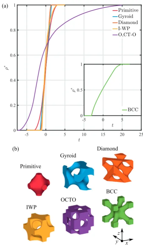
0 to be void. Varying the param-etertshifts the position of the solid-void boundary, creating larger or smaller solid regions, thus allowing us to control the solid volume fraction of the lattice,q∗. By correlatingq∗andtfor each cell type, we can use Eqs. (7a)–(7d) and (8) to generate lattices with a predefined volume fraction.Fig. 1(a) showsq∗(t) curves for the lattice cell types examined in this work, while the unit cells are presented inFig. 1(b). To design a lattice structure with a predefined volume fraction actu-ally requirest(q∗) rather thanq∗(t), but this is trivial once the two parameters are correlated with reasonable accuracy. A noteworthy feature of the unit cells shown inFig. 1(b) is that those whose sur-face equations contain only even trigonometric functions (i.e. cosine terms) exhibit both reflection and rotation symmetry in their princi-pal axes, whereas those whose equations also contain odd functions (i.e. sine terms) do not. The latter category contains the gyroid and diamond cell types.

To the ﬁve TPMS cell types above, we add another structure, the body-centred-cubic (BCC). The BCC cell type is generally constructed by forming a three dimensional cross from straight struts [38,39], but here we use a periodic function to deﬁne an isosurface instead, in the same way that the TPMS structures are generated. The result, as illustrated inFig. 1(b), is a close approximation of the conventional strut-based structure. In fact, there are advantages to creating the BCC structure in this way. Firstly, intersections between struts are smooth curves rather than sharp corners, helping to reduce stress concentrations in these areas when the structure is subject to a load. Secondly, this method ensures the volume fraction can be made to vary smoothly throughout a latticed component, or even within a single unit cell, in precisely the same way that the volume fraction of the TPMS structures are controlled.

For the BCC structure, we must provide a new shorthand nota-tion;

C2i= cos

2ki i Li

, (9)

then we can deﬁne the isosurface;

UBCC=C2x+C2y+C2z

. . .

−2

(

CxCy+CyCz+CzCx

)

−t, (10)

withtonce again providing the means to control the volume fraction. The curve representingq∗(t) for the BCC cell type is shown in the inset toFig. 1(a).

2.2. Finite element mesh construction

We have described the general methodology for the production of hexahedral ﬁnite element (FE) meshes based on surface equations in a previous work[18]. Once thet(q∗) relationship for a given cell type

-5 0 5 10 15 20 25

0 0.2 0.4 0.6 0.8 1

-5 0 5

0 0.5 1

Primitive

x y

z Gyroid

Diamond

IWP

OCTO

BCC (a)

[image:3.595.311.540.53.443.2]

(b)

Fig. 1. (a) shows the dependence of the volume fraction (q∗) on the surface equation parameter (t) for lattice cell types examined in this work. The curve for the BCC lattice is shown in the inset, as this cell type is not part of the family of triply periodic minimal surfaces. (b) shows the examined lattice cells withq∗= 0.3.

is known, the corresponding surface equation is used to generate the 3DUﬁeld, which is based on the designer’s choice of volume fraction, cell size and cell tessellations. TheU = 0 isosurface is found and deﬁned as a boundary between solid and void phases. A hexahedral mesh for the solid elements of the structure is then obtained using the underlying Cartesian coordinate grid to specify each element’s corner nodes.

Each lattice structure and associated FE mesh was created using software developed for this purpose at the University of Nottingham. The software has the working titlethe Functional Lattice Package, or FLatt Pack, and is available for trial use upon request from the cor-responding author. Regarding the computational requirements for mesh generation, using a desktop PC with a 3.7 GHz processor, the FE mesh representing a 4× 4 × 4 diamond lattice with a total of 3.2 million elements was generated in around 50 s, with peak mem-ory usage of 2.3 GB. The equivalent 5 _× 5 _× 5 diamond lattice, with around 6.3 million elements, was generated in 90 s with peak memory usage of 4.3 GB.

2.3. Elastic modulus determination

(4)

All nodes on top plane displaced by u = L/100

x y

z (Abaqus ZSYMM

boundary codition) L

z Bottom plane

elements fixed inz L

Area, A = L

[image:4.595.320.551.55.281.2]

2

Fig. 2. A representative hexahedral mesh (of a gyroid TPMS lattice comprising 2×2×2 cells) used for FE structural analysis.

France. All elements were linear, reduced-integration solid elements; typeC3D8R, following the Abaqus labelling scheme.

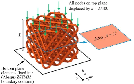
The lattice models were subjected to compressive displacements at the nodes of their top planes equivalent to 1% of the height of each structure, as illustrated inFig. 2. TheZSYMMboundary condition was applied to the elements on the top and bottom surfaces of each lattice model. This constrained these elements to translation in thexyplane only and rotation around thezaxis only.

The elastic modulus of each lattice structure was found from

Elatt.= FL

Au, (11)

whereFis the total reaction force at the top surface of the structure (a requested output from the FEA solver),Lis original height of the lattice,Ais the cross-sectional area of the lattice domain anduis the displacement of the top surface in the loading direction, which here is always equal toL

/

100. To ensure the results presented here are generally applicable for structures composed of a range of materials with differing elastic moduli, we used Eq. (2) to obtainE∗for each of the examined lattice models.

Throughout this investigation we assigned an elastic modulus of 1.8 GPa to the solid elements in our FE models. This was obtained from measurements of stress-strain curves of EOS PA2200 (nylon 12) dog-bone specimens made by selective laser sintering (SLS). We chose this elastic modulus because we have previously investigated lattice structures made by this method in this material [2,18] and it is quite commonly used in AM research. However, because we have used an entirely elastic approximation in our FE analysis, and because we have chosen to present the normalised elastic modulus,

E∗, throughout this work, the exact numerical value of the element modulus does not have a major bearing on our results or conclusions.

2.4. Finite element mesh convergence and lattice cell tessellation

Here we present a preliminary investigation into the numerical convergence of elastic moduli obtained from lattice structure FEA. We address an outstanding question in lattice simulation: how many unit cells must be tessellated in a structure for it to take on the behaviour of a homogeneous porous material? In answering this, we are able to use a reliable modelling approach to investigate other important aspects of lattice performance in the following sections.

In this investigation into mesh convergence we have consid-ered the relative elastic modulus evaluated along thezaxis, or the

1 × 1 × 1

2 × 2 × 2

3 × 3 × 3

4 × 4 × 4

5 × 5 × 5

x

y

z

Fig. 3. Diamond lattice structures comprising 1×1×1 to 5×5×5 unit cells with volume fraction,q∗= 0.3.

crystallographic [001] direction, of each lattice structure. This is represented asE∗_[001].

Fig. 3shows a range of diamond lattice structures with cell tessel-lations ranging from 1×1×1 to 5×5×5. Their volume fraction was set at 0.3, which was achieved using Eq. (7c) withtequal to₋0.4824. Hexahedral FE meshes with varying element sizes were constructed using the method outlined inSection 2.2and analysed according to Section 2.3. TheE_[001]∗ results for these diamond lattice structures are given inFig. 4.

Fig. 4(b) provides a clearer picture of the trends inFig. 4(a) by normalising the number of elements in each FE model by the number of lattice cells it contains; i.e. the number of elements in the 5×5×5

103 104 105 106 107

0 40 80

0 2 4 6 8 10

104 0

[image:4.595.51.287.56.204.2]

40 80

[image:4.595.323.550.469.708.2]

(5)

model is divided by 125 and so on. Thus, total mesh sizes which range from around 600 to 6,000,000 elements for the 1×1×1 to 5×5×5 lattice models can be expressed as between around 600 and 90,000 elements per unit cell.

We found that mesh sizes of around 50,000 elements per unit cell were suﬃcient to reduce the FE discretisation errors to insigniﬁ-cant levels. This is in good agreement with the work of Montazerian et al.[29], who examined FE mesh convergence for elastic modulus in several TPMS unit cells. Montazerian et al. determined a power law describing the percentage change in the FE result for a given number of elements in the unit cell model. This allows us to predict the num-ber of elements per unit cell required for a 1% change in the relative elastic modulus based on Montazerian et al.’s data; it is∼64,000.

In addition to FE mesh convergence behaviour, fromFig. 4it can also be seen that diamond lattice structures with fewer cells have the lowest moduli. InFig. 5we presentE_[001]∗ for the diamond lattice models shown inFig. 3. Accompanying the data is a ﬁt obtained with the exponential function

E∗=aexp(−bm) +E∗_∞, (12)

wheremis the lattice order, denoting the number of cell repetitions in the lattice model in each direction (i.e.m _× m _× mcell repeti-tions), andaandbare scaling factors.E∗_∞provides the upper bound of the relative elastic modulus as the number of cells in the lattice approaches inﬁnity. For the diamond lattice withq∗ = 0

.

3, loaded in the [001] direction, E_∞∗ was found to be (60

.

9±0

.

2) × 10−3_.

This value is important, as it represents the relative elastic modu-lus that would be assigned to this particular lattice structure if it were to be approximated as a homogeneous porous solid, or contin-uous medium. Such an approximation is a necessary step in efforts to combine TO algorithms with lattice structure design, as discussed inSection 1.

Fig. 5shows that the converged modulus of the 4 × 4× 4 cell diamond lattice was just 0

.

4%below the value ofE∗_∞. Our results therefore indicate that, for the purpose of elastic modulus determi-nation, there is no beneﬁt to modelling cubic lattice structures with greater than 43_{or 5}3_{cells, while the disadvantage of modelling only a}

single unit cell is that it may underestimate the modulus by over 15%. With this in mind, all the following results in this report concern-ing lattice cell type, cell orientation, volume fraction and functional grading, were obtained using lattice structures with the 4×4×4 cell conﬁguration. This provides the additional beneﬁt of reduced com-putational cost in the FE simulations compared with larger lattice models.

The incrementally increasing modulus of Fig. 5 is due to the diminishing effect of those cells at the boundaries of the structures.

1 2 3 4 5

[image:5.595.304.554.56.297.2]

50 54 58 62

Fig. 5. Evolution of relative elastic modulus along the cellular [001] direction with increasing number of diamond lattice unit cells withq∗= 0.3.

1 × 1 × 1

3 × 3 × 3

5 × 5 × 5

Lattice

cells

z-displacement

von Mises stress

x z

(b)

(a)

Fig. 6.Evolution of thez-displacement (a) and von Mises stress distributions (b) with increasing numbers of diamond unit cells withq∗= 0.3. These results were obtained using the boundary conditions illustrated inFig. 2.

With larger numbers of cells in the lattice, smaller proportions of them are situated at the boundaries and their contribution to the stiffness of the whole structure is reduced. This leads to the devel-opment of homogeneity in the structural deformation and stress distribution, thus providing a more accurate description of cell defor-mation as if it were part of a homogeneous porous solid. This effect is illustrated inFig. 6, which shows the evolution of thez -displacement and von Mises stress distributions for a range of lattice cell tessellations.

0 2 4 6 8 10

104 0

50 100 150 200 250

[image:5.595.312.540.467.691.2]

0 50 100 150

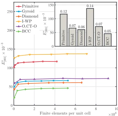
[image:5.595.44.275.558.718.2]

(6)

Using the above result concerning the number of unit cells to be tessellated to approximate a homogeneous porous solid, we turn our attention to the various TPMS lattice types introduced inSection 2.1.

E∗_[001] for primitive, gyroid, diamond, I-WP, O,C-TO and BCC lattice structures with 4×4×4 cells and volume fraction equal to 0.3 are shown inFig. 7. As inFig. 4(b), the number of elements in each model is normalised by the number of unit cells it contains, which in this case is 64 for every structure.

Fig. 7shows that the lattice cell geometry has a large effect on the relative elastic modulus. This has signiﬁcant implications for lattice design strategy. For example,E∗_[001]for the I-WP lattice structure is close to three times greater than that of the BCC structure with the same volume fraction. This would guide the designer of an AM com-ponent to select an I-WP lattice over a BCC lattice if their requirement was to maximise stiffness in one direction. This result is simpliﬁed in the inset toFig. 7, where the elastic modulus along the cellular [001] direction of each lattice type is compared.

3. Results

Having addressed the issues of FE mesh resolution and lattice cell tessellations inSection 2.4, our main results are organised into two sections. In the ﬁrst, we extend our elastic moduli analysis to include different lattice orientations and volume fractions. This yields a suc-cinct set of numerical results relating to the Gibson-Ashby scaling law of Eq. (1). Such results form a crucial part of any homogenisation approach to lattice design, enabling the development of combined TO-lattice design methods of the kind outlined inSection 1.

Secondly, we lay out our ﬁndings concerning lattice functional grading, where the volume fraction and cell type are varied through-out the structure. We demonstrate how the Gibson-Ashby scaling laws can be used to approximate the stiffness of arbitrarily graded lattices structures, and we highlight one approach to the problem of reduced strut thickness that can arise when one cell type transitions into another.

3.1. Cell type, orientation and volume fraction

In this section we apply the results fromSection 2.4 concern-ing cell tessellation and FE mesh convergence to the examination of relative elastic modulus for different lattice cell types, orienta-tions and volume fracorienta-tions. Each lattice structure examined here is a 4×4×4 arrangement of unit cells, with each cell containing∼50,000 elements in the FE model.

Lattice structures with volume fractions from 0.2 to 0.5 were obtained using Eqs. (7a)–(7d), (8) and (10), and theq∗–trelationships presented inFig. 1. To obtain relative elastic moduli along the [111] and [011] directions for each structure, a rotation matrix of the form

R(h) =

cos(h) −sin(h) sin(h) cos(h)

, (13)

was applied to the Cartesian coordinate system prior to the imple-mentation of the TPMS equations. To rotate a lattice structure to provide the [011] direction for loading in FEA, the rotation matrix was applied in theyzplane usingh = p

/

2. For the [111] direction, thep

/

2 rotation was applied in theyzplane followed by a rota-tion of 35

.

26◦in thexzplane. Rotated lattice structure models for FE simulation are illustrated inFig. 8.

Fig. 9shows theE∗(q∗) curves for three of the examined lattice types (for brevity we have chosen to display only the curves relat-ing to the primitive, diamond and BCC lattices). TheE∗(q∗) data were ﬁtted with a modiﬁed form of Eq. (1); this was

E∗(d) =C1(d)q∗n(d)+E∗0(d), (14)

x y

z

[001]

[111] _[011]

[001] loading [111] loading [011] loading

Nodes on top plane displaced by L/100

L

[image:6.595.313.560.56.277.2]

Diamond unit cell

Fig. 8. [001], [111] and [011] orientations of the lattice structures with respect to the applied compressive load.

wheredindicates that these properties are directionally dependent, that is, they vary according to the orientation of the applied dis-placement with respect the internal axes of the lattice cell. TheE∗₀(d) term accounts for systematic uncertainties in the determination of

E∗by the FE method employed here, and provides a necessary offset fromE∗ = 0 in cases where the cell geometry prohibits structural connectivity at low volume fractions.

This aspect of lattice structure design applies to all cell types, TPMS or otherwise, to some extent, though in general it only inhibits the design of very low volume fraction structures. The effect is more pronounced when there is a large disparity between the thinnest and

0 0.1 0.2 0.3

0.15 0.25 0.35 0.45 0.55

0 0.1 0.2 0.3

0 0.1 0.2

0.3 Diamond Primitive

[image:6.595.317.557.458.699.2]

BCC

(7)

= 0.24

*

= 0.22

*

= 0.20

*

= 0.18

*

Decreasing volume fraction

[image:7.595.315.542.53.286.2]

Termination

of structural

connectivity

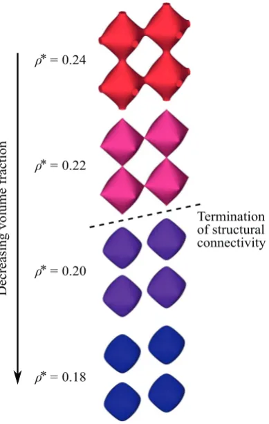
Fig. 10. A 1×2×2 lattice of primitive cells with volume fraction from 0.18 to 0.24. The structure becomes unconnected, and therefore non-load-bearing, when the volume fraction is reduced below around 0.22.

thickest structural features in the cell geometry. In these cases, when the volume fraction is lowered below a certain threshold, which will be different for all cell types, the thinnest features degrade entirely, leaving unconnected solid sections. The decomposition of the prim-itive lattice structure into isolated regions at low volume fraction has previously been observed by Yang et al.[40]An example of this behaviour can be seen inFig. 10, which shows a small primitive lat-tice withq∗ = 0

.

18–0.24. It is clear fromFig. 10that belowq∗∼

0

.

22 the primitive lattice lacks structural connectivity and therefore cannot be load-bearing. This explains the intersection of theE∗(q∗) curves for this lattice structure with the abscissa axis inFig. 9at aroundq∗= 0

.

2–0.24.

This connectivity issue precluded the possibility of determining

E∗ (q∗ = 0

.

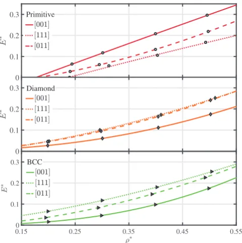
2) for the primitive lattice structure in each of the three cell orientations. Instead, the lowest volume fraction examined for the primitive lattice was 0.24. The O,C-TO unit cell is similarly restricted to volume fractions above 0.24, so the lowest volume fraction examined for this lattice was 0.25.

TheE∗(q∗) curves inFig. 9demonstrate that the orientation of lat-tice cells with respect to the applied displacement has a signiﬁcant

0.2

0.3

0.4

0.5

[image:7.595.63.258.57.364.2]

0

0.1

0.2

0.3

Fig. 11. E∗(q∗) resulting from the Gibson-Ashby factors given inTable 1. The stiffest and most compliant cases atq∗= 0.3 are highlighted.

effect on the relative elastic modulus. For example, atq∗ = 0

.

3,

E∗_[001] for the primitive lattice structure is almost twice as large as

E∗_[111]. Another interesting feature is that, for the diamond structure, theE∗_[111](q∗) andE∗_[011](q∗) curves are almost identical, and both rep-resent much higher moduli than theE∗_[001](q∗) curve.Table 1contains the Eq. (14) ﬁtting results for all six of the examined TPMS lattice structures for the [100], [111] and [011] cell orientations.

TheE∗(q∗) curves for every lattice cell type and loading direction examined in this work are presented together inFig. 11. We have highlighted the two cases which represent the stiffest and most com-pliant responses to compressive loading at a volume fraction of 0.3; these are the I-WP lattice in the [001] orientation and the BCC lattice in the [001] orientation, respectively. There is approximately a factor of three difference in the elastic moduli of these conﬁgurations. The remaining curves ofFig. 11serve as a clear illustration of the range of elastic moduli that can be achieved through appropriate selection of lattice cell type, cell orientation and volume fraction.

3.2. Lattice functional grading

In this section we explore two interesting aspects of lattice structure design; volume fraction grading and cell type grading, or hybridisation. Both may be used to facilitate functional grading, that is, the variation of a particular property, often but not necessarily mechanical, throughout a component. This is one way to provide the most materially-eﬃcient solution for a given loading condition, such as when unpenalised topology optimisation results are used as

Table 1

Numerical constants derived by applying Eq. (14) to the relative elastic moduli of the lattice structures.

[001] [111] [011]

C1 n E0∗ C1 n E∗0 C1 n E∗0

Primitive 0.92 1.0 −0.172 0.65 0.8 −0.198 0.90 1.8 −0.043 Gyroid 1.02 2.4 0.002 0.78 1.6 −0.004 0.86 1.9 −0.003 Diamond 0.75 2.1 0.003 0.77 1.6 −0.013 0.83 1.8 −0.001 I-WP 0.76 1.6 0.032 0.99 1.9 −0.044 1.16 2.3 −0.002 O,C-TO 1.22 1.9 −0.056 0.91 1.3 −0.126 1.00 1.4 −0.113

[image:7.595.31.553.659.744.2]

(8)

a guide for material layout [22,23]. Alternatively, functional grad-ing can provide novel behaviour, such as layer-by-layer structural collapse [2,41] and tailorable impactor deceleration under dynamic loading[42].

3.2.1. Volume fraction grading

Volume fraction grading is achieved with a simple adjustment to the surface equations introduced inSection 2.1. To allow the vari-ation of the volume fraction throughout the lattice, we replace the formerly single-valuedtin Eqs. (7a)–(7d), (8) and (10) with a new, spatially-dependent parameter,t(x,y,z). This has the same role ast, in that it controls the position of the boundary between solid and void phases of the structure, and we can apply the same relationships presented inFig. 1to control the volume fraction.

Taking, for example, Eq. (7c), which provides the isosurface for the diamond lattice, we create a new surface equation of the form

UD=SxSySz+SxCyCz+CxSyCz

. . .

+CxCySz−t(x,y,z)

.

(15)

t(x,y,z) is now an arbitrarily deﬁned spatial distribution, with its value at any point in space determined by the correspondingt(q∗) relationship for the diamond lattice.

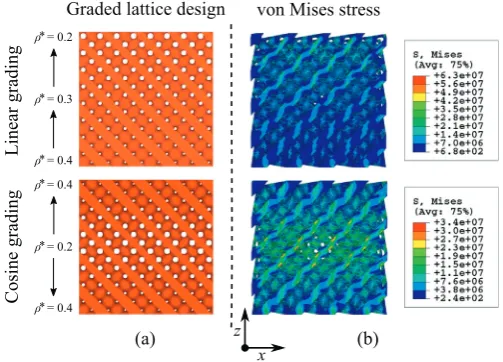
InFig. 12we illustrate how this can be used to generate novel graded structures.Fig. 12(a) shows two diamond lattice structures with different types of volume fraction grading. In the ﬁrst example, the grading is speciﬁed by a linear function of the lattice height, with

q∗ = 0

.

4 at the base andq∗= 0

.

2 at the top of the structure. In the second example, a single oscillation of the cosine function is used; the oscillation has a meanq∗ = 0

.

3 and a magnitudeq∗ = 0

.

1. Formally, and deﬁning the structure’s height to be 1, these are given by

q∗_lingrad(z) = 0

.

4−0

.

2z, (16)

and

[image:8.595.42.294.518.699.2] [image:8.595.322.550.552.718.2]

q∗_cosgrad(z) = 0

.

3 + 0

.

1 cos(2pz)

.

(17)

Fig. 12(b) shows the von Mises stress distributions in these graded structures when a compressive displacement is applied in the z

Linear grading

von Mises stress

x

z

_(b)

(a)

Graded lattice design

Cosine grading

ρ*= 0.4

ρ*= 0.2

ρ*= 0.3

ρ*= 0.4

ρ*= 0.2

Fig. 12. Diamond lattice structures with linear volume fraction grading (above) and cosine volume fraction grading (below). (a) shows the material layout, while (b) shows the resulting von Mises stress distributions when the structures are subject to a compressive load.

direction to their top surfaces - the same boundary condition shown inFig. 2and used throughoutSections 2.4and3.1. The regions of the graded lattice structures with the lowest volume fraction are seen to develop the highest stresses. The cellular struts or members in these regions are likely to buckle or yield at lower net strains compared to those in higher volume fraction regions, leading to premature failure of the whole structure. In comparison, the stresses in the 3×3×3 and 5 _× 5 _× 5 structures ofFig. 6, which have the same average volume fraction as those inFig. 12(b), are well distributed, which is more likely to provide the predictable deformation behaviour of cellular solids.

Before examining the elastic moduli of the examples inFig. 12, we introduce a relevant result concerning the calculation of total stiff-ness,ktot, of a graded structure. For a series arrangement ofnsprings

we have

1

ktot = n

i=1

1

ki

, (18)

where ki is the stiffness of each spring. Applying this to a struc-ture composed ofnmaterials with moduli,Ei, stacked in the same

direction as an applied load, we obtain

1

Etot=

1

n n

i=1

1

Ei

, (19)

for the total elastic modulus of the system. This assumes the cross-sectional area,A, remains constant throughout the loading direction and the thickness of each material isL

/

n. This case is illustrated in Fig. 13, in which we include theq∗andE∗nomenclature to highlight that these results may be applied to graded lattice structures.

Assuming a continuous elastic modulus variation along the load-ing direction, which here isz, rather than a series of discrete slices, we can use an integral form of Eq. (19):

1

E∗_tot= L

0

1

E∗₍_z₎dz, (20)

whereE∗(z) is the distribution of the lattice structure’s relative elas-tic modulus alongz. For the graded structures shown inFig. 12we do not explicitly knowE∗(z), and this will be true in general, but we knowq∗(z) and can ﬁndE∗(q∗) from Eq. (14) and the numerically

Area, A

L

L/n

Cell type 1, *1, E1* Cell type n, *n, E*n

Material 1, E1 Material n, En

Applied load

(9)

determined factors in Table 1. Therefore, a more useful form of Eq. (20) for lattice structures is

1

E∗_tot = L

0

1

C1q∗₍_z₎n₊_E∗ 0

dz

.

(21)

To calculate solutions for the linear and cosine graded example structures ofFig. 12we can substitute Eqs. (16) and (17) forq∗(z), and use the numerical results inTable 1. For the diamond structures shown inFig. 12, we then have

1

E∗_lingrad = 1

0

1

0

.

75(0

.

4₋0

.

2z)2.1_{+ 0}

_.

₀₀₃dz, (22)

and

1

E∗_cosgrad = 1

0

1

0

.

75

(

0

.

3 + 0

.

1 cos(2pz)

)

2.1+ 0

.

003dz, (23)

for the linear and cosine graded lattices, respectively. Note that the integral limit is 1, as deﬁned for the simpliﬁcation of the volume fraction grading, i.e. Eqs. (16) and (17).

The numerical solutions for the relative elastic moduli of these structures are provided in Table 2, where the results obtained directly from FE models of the graded structures are also given. The results are in extremely good agreement, with the values pre-dicted from the integration method underestimating the FE moduli by just a few percent. This demonstrates that the elastic moduli of graded volume fraction lattices can be accurately predicted from prior knowledge of their spatial volume fraction distributions and

E∗(q∗) relationships.

[image:9.595.314.541.58.220.2]

Furthermore, if the spatial volume fraction distribution is not known or is not expressible in an explicit form (such as Eqs. (16) and (17) used above), a general numeric summation with suﬃcient terms,n, could provide a reasonable approximation of the elastic modulus by applying Eq. (19). When the linearly graded structure of Fig. 12is approximated as having just three lattice layers withq∗n=

0

.

2, 0.3 and 0.4, the resulting relative elastic modulus is 48

.

0×10−3_,

which is 14% less than the FE result. The discrepancy decreases to 10% when the numerical summation uses ﬁve terms instead of three.

3.2.2. Cell type grading, or hybridisation

We can make use of two or more of the surface equations from Section 2.1 to create lattice structures in which one cell type transitions into another. These have come to be known as multi-morphology, or hybrid lattice structures [43,44]. The transi-tion between cell types may be abrupt ‘step’ changes, or may be more broad, taking place over length scales of one or more unit cells. The second case will give rise to cell hybridisation, where the mor-phology of intermediate cells lies between those of the two known cell types. The width of the transition region, and the amount of cell hybridisation, is deﬁned by the choice of weighting distribution used to allocate cell types to different regions of the lattice structure. Such multi-morphology cellular structures based on TPMS equations have previously been designed and fabricated by Yoo and Kim [43],

0 0.2 0.4 0.6 0.8 1

Lattice type 1

Lattice type 2

[image:9.595.33.283.189.275.2]

Hybrid region

Fig. 14.The cell type weighting distribution for a hybrid of two lattice types may be described by the sigmoid function with variable transition width.

and Yang et al.[44], with the latter authors describing the general methods underlying their design.

In the simplest case, where we consider grading between just two cell types, we have

Uhyb=aU1+ (1−a)U2, (24)

whereais the cell type weighting distribution, andU1andU2are

any functions describing lattice solid-void boundaries, such as those in Eqs. (7a)–(7d), (8) and (10). Using these, we can determine the

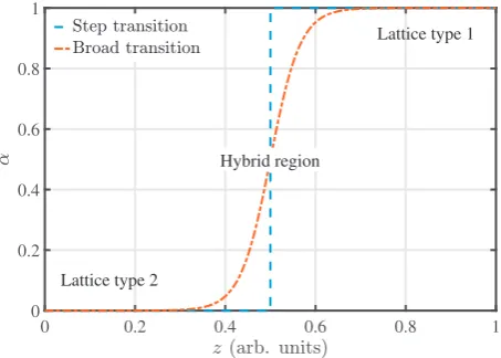
Uhyb = 0 isosurface to construct the resulting hybrid lattice.ais

a spatial function that varies between 0 and 1, with the sigmoid function being identiﬁed by Yang et al.[44]as a convenient and eﬃ-cient example. It is capable of describing step transitions between lattice types, as well as broad transitions of arbitrary width; see, for example,Fig. 14, in which the sigmoid function along a single direc-tion is presented. The three dimensional form of the sigmoid funcdirec-tion is

a(x,y,z) = 1

1 +e−kG(x,y,z), (25)

withG(x,y,z) being a spatial coordinate set describing the shape of the boundary between lattice regions andkdeﬁning the transition width. The transition between lattice regions occurs atG(x,y,z) = 0, so simple cases of planar transitions can be achieved quite readily by, for example, subtracting an intermediate value from all coordi-nates in eitherx,yorz.ktakes values greater than zero, with larger values of kproviding more narrow transition regions. Whenk is extremely large compared to the dimensions of the lattice structure, the sigmoid function closely approximates a step transition.

InFig. 15we present two example hybrid structures, where the transition between regions of different lattice type is achieved with a sigmoid function ofzonly. With respect to Eq. (25), this is achieved by choosingG(x,y,z) = 0 to be a ﬂat plane at mid-height in the structure. In both cases, the volume fraction is set to 0.3 everywhere. These illustrate two outcomes of hybrid lattice design to which we wish to draw attention. InFig. 15(a), where the diamond cell type

Table 2

Relative elastic moduli of graded volume fraction diamond lattice structures.

E∗from graded FE model×10−3 _E∗_from_E∗₍_q_∗_{) integration}_×₁₀−3 _{Diff. (%)}

Linear grading (q∗= 0.2–0.4) 55.9 53.8 −4

[image:9.595.31.554.709.745.2]

(10)

Gyroid region

Diamond region Step transition

(a)

x y

z Gyroid region

Primitive region Hybrid region (b)

[image:10.595.46.292.56.272.2]

Front view

Fig. 15. Diamond-gyroid hybrid lattice with a step boundary (a) and primitive-gyroid hybrid lattice with a broader transition (b). Both are achieved using a sigmoid function ofz.

undergoes a step transition into the gyroid cell type, we ﬁnd the material distribution in thezdirection to be fairly continuous; that is, there is no signiﬁcant discontinuity of load-bearing material from the base of the structure to its top. We can apply Eq. (19) and the results fromTable 2to approximate the relative elastic modulus of this hybrid structure, withEi being the moduli of the diamond and

gyroid lattices. We obtain a relative elastic modulus of 61

.

0×10−3_,

which is in excellent agreement with the result from the FE model. These numerical results are given inTable 3.

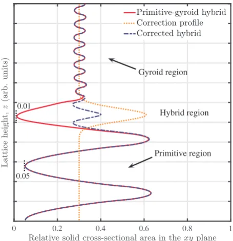
Conversely, for the primitive-gyroid hybrid lattice shown in Fig. 15(b), the volume fraction of the hybrid region is severely dimin-ished compared to the rest of the structure. This is shown more clearly in thexzandyzplanar views ofFig. 16, and also in the analy-sis of the hybrid structure’s solid cross-sectional area in thexyplane inFig. 17.

InFig. 17we see that the periodic variation of the primitive lattice region’s solid cross-sectional area is between 5% and 63% of the area of the structure. In the hybrid region, this is reduced to just 1%, con-stituting a relative reduction in load-bearing area of around 80%. This region will therefore be signiﬁcantly less stiff, and will be subject to considerably higher stress, than the adjoining regions. This is a con-sequence of the hybridisation between primitive and gyroid cells in this layout, and results in structural weakening at the transition.

The effect of the reduced load-bearing area in the hybridised region becomes apparent when we apply the elastic modulus sum-mation approach introduced above. Eq. (19) predicts the relative elastic modulus of the primitive-gyroid hybrid to be 80

.

5 × 10−3_,

but this is over 25% higher than the elastic modulus of that structure determined from the corresponding FE model. The elastic modulus is overestimated by Eq. (19) because it does not account for the low volume fraction transition region.

Uncorrected G-P hybrid Corrected G-P hybrid

Front view

Side view

Thickenned hybrid region to avoid structural weak points.

[image:10.595.321.548.57.262.2]

z x,y

Fig. 16. Planar views of the primitive-gyroid hybrid lattice. On the left is the original structure with its weakened central section. On the right is the same hybrid structure following the application of a volume fraction correction step.

To counteract this undesirable effect of cell hybridisation, we propose a new design approach in which the volume fraction of a hybrid lattice is analysed and ‘corrected’ in the transition region. This approach incorporates spatial volume fraction control, as introduced inSection 3.2.1, as a tool to avoid structural weak points, and produce a hybrid lattice design which can be more accurately modelled with Eq. (19). This approach is outlined generally inFig. 18, which includes references to other ﬁgures in which each step of the approach is illustrated.

In the simple case of the primitive-gyroid hybrid structure in Figs. 15(b) and16, in which the cell transition occurs in thez direc-tion only, our volume fracdirec-tion correcdirec-tion approach can be applied quite easily. First, the primitive-gyroid hybrid is generated using a target volume fraction which is 0.3 everywhere. Next, we examine the solid cross-sectional area of the lattice in thexyplane (seeFig. 17) and identify a region where this is far lower than elsewhere. The solid cross-sectional areas are ﬁt with a Gaussian function of the lattice height (z). We then create a new volume fraction distribution for the whole structure based on this Gaussian function, but with its mag-nitude inverted; inFig. 17this can be seen as a peak centred around the mid-height, with a maximum value just over 0.6. In 3D, this new volume fraction distribution,q∗corr(x,y,z), is equal to 0.3 almost

every-where, but it features a band, or sheet, of higher volume fraction at mid-height in the structure.

In the ﬁnal step the primitive-gyroid hybrid lattice is re-generated using q∗corr(x,y,z). The effect, as shown inFig. 16, is to

thicken the cell struts in the hybrid region, providing a more uniform transition between the primitive and gyroid lattice types.

[image:10.595.40.573.694.744.2]

The volume fraction correction process has a marked impact on the mechanical performance of the primitive-gyroid hybrid lattice compared to its original form. First, the hybrid region is no longer

Table 3

Relative moduli of primitive (P)-gyroid (G) lattice and diamond (D)-gyroid (G) hybrid structures.

E∗from hybrid FE model×10−3 _E∗_from_E∗

icell summation×10−3 Diff. (%)

D-G hybrid lattice (step transition) 61.1 61.0 <1

P-G hybrid lattice 63.6 80.5 27

(11)

0 0.2 0.4 0.6 0.8 1

Hybrid region Gyroid region

Primitive region 0.01

[image:11.595.44.272.56.292.2]

0.05

Fig. 17. The cross-sectional load bearing area of the primitive-gyroid hybrid structure before and after volume fraction correction. (For interpretation of the references to color in this ﬁgure legend, the reader is referred to the web version of this article.)

associated with low stiffness and high stress. This is clear from the von Mises stress distributions presented inFig. 19. Second, the rela-tive elastic modulus of the corrected hybrid structure is more accu-rately described by the summation method of Eq. (19). The results given inTable 3show that Eq. (19) nowunderestimates the elastic modulus obtained from the FE model, and by a much smaller margin than for the uncorrected hybrid. In the context of lattice structure design, this is a more preferable situation, and the discrepancy could be reduced further by using a more sophisticated correction function than the single Gaussian peak used in this example. Furthermore, the four step procedure ofFig. 18could be modiﬁed into an iterative loop, whereq∗corris redeﬁned asq∗and passed back to step 1. This

has the potential to virtually eliminate the discrepancy between the target stiffness and the actual stiffness of the hybrid structure.

Analyse the hybrid structure to identify regions of unusually low volume fraction.

2

Generate hybrid lattice with

t( ) for each cell type.*

1

*

Create a corrected volume fraction distribution, , with increased volume fraction in regions identified in step 2.

corr

3

with t( ) for each cell type. Generate a corrected hybrid lattice

*

corr

4

see Figure 15

see Figure 17 (red solid line)

see Figure 17 (orange dotted line)

see Figures 16 and 19

Fig. 18. Proposed approach for the design of hybrid lattice structures. This includes analysis and correction steps which identify and eliminate structurally weak lattice regions. On the right are indicated the ﬁgures in this paper which these steps are illustrated.

x

z

(a)

(b)

Fig. 19.Planar views of the von Mises stress distributions for the primitive-gyroid hybrid structure. (a) shows the original hybrid, while (b) shows the structure following the application of a volume fraction correction step.

4. Discussion

We present results inSection 3.1 that are highly valuable to designers of lattice structures. These are the Gibson-Ashby coeffi-cients relating relative modulus and volume fraction for a range of surface-based cell types. As demonstrated inSection 2.4, these results are based on robust, converged modelling which accounts for FEA mesh convergence and lattice homogenisation, i.e. mod-elling a sufficient number of cell tessellations. Our FEA model based on a single unit cell yielded a stiffness 16%lower than an upper bound representing the homogeneous, semi-infinite case. This indi-cates that future studies should not rely on the analysis of a single unit cell if they aim to determine useful material models or design rules.

Such results concerning the increase in mechanical properties of AM fabricated cellular structures with decreasing cell size have pre-viously been reported by Yan et al.[45]and Bose et al.[46]. However, those studies did not focus on the issue of mechanical property con-vergence with cell tessellations, so their ﬁndings in this regard can not be used in the development of general lattice design rules.

Fig. 9andTable 1show how the Gibson-Ashby exponent,n, varies according to cell type and orientation with respect to the applied load. Our previous work[18]and that of others [19,20] has indicated thatnclose to unity represents stretching-dominated elastic defor-mation in this type of lattice structure, whilencloser to 2 and above represents bending-dominated behaviour. It is therefore interesting to examineTable 1and note the wide range of mechanical responses one might expect from the examined lattice structures and loading orientations. For example, we expect the primitive lattice to exhibit stretching-dominated deformation behaviour when loaded along the [001] direction, but be more prone to bending when loaded along [011]. This is supported by a consideration of the primitive cell’s geometry, with its connecting members being aligned along001 directions.

[image:11.595.302.553.59.240.2] [image:11.595.46.271.544.703.2]

(12)

also possesses large mechanical anisotropy between its [001], [111] and [011] cellular orientations, with the difference in stiffness along [001] and [111] being a factor of 2.5 atq∗ = 0

.

3, so this may not be the best cell type for cases including the possibility of off-axis loading. Our analysis indicates that the diamond lattice type has the lowest overall mechanical anisotropy.

Regarding the functional grading examined inSection 3.2, a few points are worthy of additional discussion. First, we presented only simple examples of lattice volume fraction grading. We did so in order that they serve as straightforward test cases for the modulus summation and integration methods of Eqs. (19) and (20), respec-tively. These equations were able to accurately predict the moduli of the graded structures, a result which may be profoundly useful in future AM lattice design. Eq. (19) or (20) can be used in con-junction with the Gibson-Ashby parameters ofTable 1to design a graded lattice structure to meet a particular stiffness requirement in any of the001,111or110loading directions, while also exhibit-ing a predictable and tailorable collapse process. For example, it has previously been shown that linearly graded BCC lattices undergo sequential layer collapse when loaded along the grading direction [2,41], with the advantage of larger compressive energy absorption compared to non-graded equivalent structures. Our ﬁndings indicate a means to achieve the same sequential collapse, but with an initial stiffness which is chosen to satisfy a given load condition.

InSection 3.2.2we proposed a new design approach enabling the construction of multi-morphology hybrid lattice structures which uniquely avoids an undesirable consequence of cell hybridisation. Speciﬁcally, depending on the choice of lattice types and the width of the transition between them, cell hybridisation can create regions of extremely low volume fraction. These will be much less stiff than the surrounding regions, leading the structure to under-perform in load-bearing applications. They will also experience much higher stress, and are therefore likely to fail prematurely. In our hybrid lattice design approach, such regions are identiﬁed and their vol-ume fractions corrected, so that the resulting structure behaves more predictably.

We demonstrated our approach with a fairly simple example; see Figs. 16,17and19. In cases where the transition between lattice types is not governed by a simple spatial function along one direc-tion, or when more than two lattice types are hybridised in the ﬁnal structure, our volume fraction correction approach will be more dif-ﬁcult to implement, but it will be fundamentally the same as that laid out inFig. 18. A general solution would use a three dimensional volume fraction analysis, with the resultingq∗corr(x,y,z) potentially

requiring a large number of perturbations from the originalq∗(x,y,z) to eliminate the structural weak points. Even so, since lattice struc-ture design is by necessity conducted using computers, algorithms to determineq∗corr(x,y,z) for arbitrary lattice hybridisation cases could

be developed quite straightforwardly.

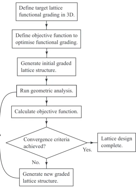
Our general approach for functionally graded lattice design is set out inFig. 20. This incorporates an objective function, the purpose of which, much like within topology optimisation, is to check whether the material distribution of the structure is consistent with the spec-iﬁed functional grading. If it is not, the hybrid correction ofFig. 18, or its 3D equivalent, will be used to iteratively modify the lattice design. Once the objective function is satisﬁed to within a given tol-erance, the process is complete and the resulting structure can be taken to the next step of the design process; be it embedding in a larger component, or fabrication using an AM process.

5. Conclusions

We have investigated a range of surface-based lattice structures relevant to additive manufacturing and 3D printing. We developed a robust ﬁnite element model to determine their elastic moduli along

Define target lattice functional grading in 3D.

Define objective function to optimise functional grading.

Generate initial graded lattice structure.

Run geometric analysis.

Calculate objective function.

Lattice design complete.

Generate new graded lattice structure.

Convergence criteria achieved?

Yes.

[image:12.595.326.551.54.368.2]

No.

Fig. 20. Proposed general approach to functionally graded lattice structure design.

three loading directions, then used this model to determine useful numerical relationships between their moduli and volume fractions. The cell geometry was found to play a signiﬁcant role in deter-mining the elastic modulus, accounting for up to a factor of three difference between the stiffest lattice and the most compliant. The orientation of the lattice cells with respect to the applied load was also found to be important, but the effect was less pronounced, accounting for a factor of up to 2.5, depending on the lattice cell.

The I-WP lattice, loaded in the [001] direction, was found to be the stiffest structure across most of the range of volume fraction from 0.2 to 0.5. We can therefore recommend this lattice type be used for any application where the principal consideration is maximal stiffness along one direction. In cases where the stiffness in several loading directions are considered simultaneously, the mechanical anisotropy of the lattice cell becomes more important, and the diamond lattice, which we found to possess the lowest overall anisotropy between the [001], [111] and [011] loading directions, would be a more suitable choice.

(13)

Acknowledgments

This work was supported by the Engineering and Physical Sciences Research Council [grant number EP/P027261/1] and also by Innovate UK [project number 102665]. Thanks to Mark East, Mark Hardy and Joe White, technicians of the Centre for Additive Manufacturing.

References

[1] I. Maskery, N.T. Aboulkhair, A.O. Aremu, C.J. Tuck, I.A. Ashcroft, Compressive failure modes and energy absorption in additively manufactured double gyroid lattices, Addit. Manuf. 16 (2017) 24–29.

[2] I. Maskery, A. Hussey, A. Panesar, A. Aremu, C. Tuck, I. Ashcroft, R. Hague, An investigation into reinforced and functionally graded lattice structures, J. Cell. Plast. 53 (2) (2017) 151–165.

[3] J. Brennan-Craddock, D. Brackett, R. Wildman, R. Hague, The design of impact absorbing structures for additive manufacture, J. Phys.: Conf. Ser. 382 (1) (2012) 012042.

[4] R.E. Winter, M. Cotton, E.J. Harris, J.R. Maw, D.J. Chapman, D.E. Eakins, G. McShane, Plate-impact loading of cellular structures formed by selective laser melting, Model. Simul. Mater. Sc. 22 (2014) 025021.

[5] R.A.W. Mines, S. Tsopanos, Y. Shen, R. Hasan, S.T. McKown, Drop weight impact behaviour of sandwich panels with metallic micro lattice cores, Int. J. Impact Eng. 60 (2013) 120–132.

[6] M. Wong, I. Owen, C.J. Sutcliffe, A. Puri, Convective heat transfer and pressure losses across novel heat sinks fabricated by selective laser melting, Int. J. Heat Mass. Tran. 52 (1) (2009) 281–288.

[7] K.L. Kirsch, K.A. Thole, Pressure loss and heat transfer performance for addi-tively and conventionally manufactured pin ﬁn arrays, Int. J. Heat Mass. Tran. 108 (2017) 2502–2513.

[8] S.L. Sing, J. An, W.Y. Yeong, F.E. Wiria, Laser and electron-beam powder-bed additive manufacturing of metallic implants: a review on processes, materials and designs, J. Orthop. Res. 34 (3) (2016) 369–385.

[9] K.H. Matlack, A. Bauhofer, S. Krödel, A. Palermo, C. Daraio, Compos-ite 3D-printed metastructures for low-frequency and broadband vibration absorption, P. Natl. Acad. Sci. USA 113 (30) (2016) 8386–8390.

[10] X. Wang, P. Zhang, S. Ludwick, E. Belski, A.C. To, Natural frequency optimization of 3D printed variable-density honeycomb structure via a homogenization-based approach, Addit. Manuf. 20 (2018) 189–198.

[11] D.W. Abueidda, I. Jasiuk, N.A. Sobh, Acoustic band gaps and elastic stiffness of PMMA cellular solids based on triply periodic minimal surfaces, Mater. Des. 145 (2018) 20–27.

[12] L.R. Hart, S. Li, C. Sturgess, R. Wildman, J.R. Jones, W. Hayes, 3D printing of biocompatible supramolecular polymers and their composites, ACS Appl. Mater. Inter. 8 (5) (2016) 3115–3122. PMID: 26766139.

[13] H.N. Chia, B.M. Wu, Recent advances in 3D printing of biomaterials, J. Biol. Eng. 9 (1) (Mar 2015) 4.

[14] N.T. Aboulkhair, N.M. Everitt, I. Maskery, I. Ashcroft, C. Tuck, Selective laser melting of aluminum alloys, MRS Bull. 42 (4) (2017) 311–319.

[15] S. Gorsse, C. Hutchinson, M. Gouné, R. Banerjee, Additive manufacturing of metals: a brief review of the characteristic microstructures and properties of steels, Ti-6Al-4V and high-entropy alloys, Sci. Technol. Adv. Mat. 18 (1) (2017) 584–610. PMID: 28970868.

[16] L.J. Gibson, M.J. Ashby, Cellular Solids: Structure and Properties, Cambridge University Press. 1997.

[17] M.F. Ashby, A.G. Evans, N.A. Fleck, L.J. Gibson, L.W. Hutchinson, H.G. Wadley, Metal Foam: A Design Guide, Butterworth-Heinemann. 2000.

[18] I. Maskery, L. Sturm, A.O. Aremu, A. Panesar, C.B. Williams, C.J. Tuck, R.D. Wildman, I.A. Ashcroft, R.J.M. Hague, Insights into the mechanical properties of several triply periodic minimal surface lattice structures made by polymer additive manufacturing, Polymer (2017)

[19] X. Zheng, H. Lee, T.H. Weisgraber, M. Shusteff, J. DeOtte, E.B. Duoss, J.D. Kuntz, M.M. Biener, Q. Ge, J.A. Jackson, S.O. Kucheyev, N.X. Fang, C.M. Spadaccini, Ultralight, ultrastiff mechanical metamaterials, Science 344 (6190) (2014) 1373–1377.

[20] V.S. Deshpande, N.A. Fleck, M.F. Ashby, Effective properties of the octet-truss lattice material, J. Mech. Phys. Sol 49 (8) (2001) 1747–1769.

[21] A.G. Evans, J.W. Hutchinson, N.A. Fleck, M.F. Ashby, H.N.G. Wadley, The topological design of multifunctional cellular metals, Prog. Mater. Sci. 46 (2001) 309–327.

[22] D.J. Brackett, I.A. Ashcroft, R.D. Wildman, R.J.M. Hague, An error diffusion based method to generate functionally graded cellular structures, Comput. Struct. 138 (0) (2014) 102–111.

[23] L. Cheng, P. Zhang, J. Toman, Y. Yu, E. Biyikli, M. Kirca, M. Chmielus, A. To, Eﬃcient design-optimization of variable-density hexagonal cellular structure by additive manufacturing: theory and validation, J. Manuf. Sci. Eng. 137 (2015) 021004–021012.

[24] A. Panesar, M. Abdi, D. Hickman, I. Ashcroft, Strategies for functionally graded lattice structures derived using topology optimisation for additive manufacturing, Addit. Manuf. 19 (2018) 81–94.

[25] B. Wang, G.D. Cheng, Design of cellular structures for optimum eﬃciency of heat dissipation, Struct. Multidisc. Optim. 30 (2005) 447–458.

[26] C. Yan, L. Hao, A. Hussein, P. Young, Ti-6Al-4V triply periodic minimal surface structures for bone implants fabricated via selective laser melting, J. Mech. Behav. Biomed. Mater. 51 (2015) 61–73.

[27] D.W. Abueidda, M. Bakir, R.K.A. Al-Rub, J.S. Bergstrm, N.A. Sobh, I. Jasiuk, Mechanical properties of 3D printed polymeric cellular materials with triply periodic minimal surface architectures, Mater. Design 122 (2017) 255–267.

[28] D.W. Abueidda, R.K.A. Al-Rub, A.S. Dalaq, D.-W. Lee, K.A. Khan, I. Jasiuk, Effective conductivities and elastic moduli of novel foams with triply periodic minimal surfaces, Mech. Mater 95 (2016) 102–115.

[29] H. Montazerian, E. Davoodi, M. Asadi-Eydivand, J. Kadkhodapour, M. Solati-Hashjin, Porous scaffold internal architecture design based on minimal surfaces: a compromise between permeability and elastic properties, Mater. Design 126 (2017) 98–114.

[30] O. Al-Ketan, R. Rowshan, R.K.A. Al-Rub, Topology-mechanical property relationship of 3D printed strut, skeletal, and sheet based periodic metallic cellular materials, Addit. Manuf. 19 (2018) 167–183.

[31] H. Schwarz, Gesammelte Mathematische Abhandlungen, vol. 1 & 2. Springer, Berlin, 1885.

[32] A.H. Schoen, Inﬁnite periodic minimal surfaces without self-intersections, NASA Technical Report TN D-5541, Tech. Rep., Washington, D.C. 1970.

[33] J. Klinowski, A. Mackay, H. Terrones, Curved surfaces in chemical structure, Philos. Trans. Roy. Soc. London A 354 (1715) (1996) 1975–1987.

[34] P.J.F. Gandy, S. Bardhan, A.L. Mackay, J. Klinowski, Nodal surface approxima-tions to the P, G, D and I-WP triply periodic minimal surfaces, Chem. Phys. Lett. 336 (3) (2001) 187–195.

[35] M. Wohlgemuth, N. Yufa, J. Hoffman, E.L. Thomas, Triply periodic bicontinu-ous cubic microdomain morphologies by symmetries, Macromolecules 34 (17) (2001) 6083–6089.

[36] D.-J. Yoo, Computer-aided porous scaffold design for tissue engineering using triply periodic minimal surfaces, Int. J. Precis. Eng. Mat. 12 (1) (Feb 2011) 61–71.

[37] D. Hoffman, J. Hoffman, M. Weber, M. Trazet, M. Wohlgemuth, E. Boix, M. Callahan, E. Thayer, F. Wei., Table of Surfaces Jan 2005,http://www.msri.org/ publications/sgp/jim/papers/morphbysymmetry/table/index.htmlaccessed 1-June-2017.

[38] M. Smith, Z. Guan, W.J. Cantwell, Finite element modelling of the compressive response of lattice structures manufactured using the selective laser melting technique, Int. J. Mech. Sci. 67 (2013) 28–41.

[39] K. Ushijima, W.J. Cantrell, R.A.W. Mines, S. Tsopanos, M. Smith, An investiga-tion into the compressive properties of stainless steel micro-lattice structures, J. Sandw. Struct. Mat. 13 (2011) 303–329.

[40] N. Yang, L. Gao, K. Zhou, Simple method to generate and fabricate stochastic porous scaffolds, Mat. Sci. Eng. C 56 (Supplement C) (2015) 444–450.

[41] I. Maskery, N.T. Aboulkhair, A.O. Aremu, C.J. Tuck, I.A. Ashcroft, R.D. Wildman, R.J.M. Hague, A mechanical property evaluation of graded density Al-Si10-Mg lattice structures manufactured by selective laser melting, Mat. Sci. Eng. A-Struct. 670 (2016) 264–274.

[42] L. Cui, S. Kiernan, M.D. Gilchrist, Designing the energy absorption capacity of functionally graded foam materials, Mat. Sci. Eng. A-Struct. 507 (1) (2009) 215–225.

[43] D.-J. Yoo, K.-H. Kim, An advanced multi-morphology porous scaffold design method using volumetric distance ﬁeld and beta growth function, Int. J. Precis. Eng. Mat. 16 (9) (2015) 2021–2032.

[44] N. Yang, Z. Quan, D. Zhang, Y. Tian, Multi-morphology transition hybridization CAD design of minimal surface porous structures for use in tissue engineering, Comput. Aided Des. 56 (2014) 11–21.

[45] C. Yan, L. Hao, A. Hussein, S.L. Bubb, P. Young, D. Raymont, Evaluation of light-weight AlSi10Mg periodic cellular lattice structures fabricated via direct metal laser sintering, J. Mater. Process Tech. 214 (2014) 856–864.