Identification of single-input–single-output quantum linear systems
Matthew Levitt*and M˘ad˘alin Gut¸˘a
School of Mathematical Sciences, University of Nottingham, University Park, NG7 2RD Nottingham, United Kingdom (Received 3 October 2016; published 22 March 2017)
The purpose of this paper is to investigate system identification for single-input–single-output general (active or passive) quantum linear systems. For a given input we address the following questions: (1) Which parameters can be identified by measuring the output? (2) How can we construct a system realization from sufficient input-output data? We show that for time-dependent inputs, the systems which cannot be distinguished are related by symplectic transformations acting on the space of system modes. This complements a previous result of Gut¸˘a and Yamamoto [IEEE Trans. Autom. Control61,921(2016)] for passive linear systems. In the regime of stationary quantum noise input, the output is completely determined by the power spectrum. We define the notion of global minimality for a given power spectrum, and characterize globally minimal systems as those with a fully mixed stationary state. We show that in the case of systems with a cascade realization, the power spectrum completely fixes the transfer function, so the system can be identified up to a symplectic transformation. We give a method for constructing a globally minimal subsystem direct from the power spectrum. Restricting to passive systems the analysis simplifies so that identifiability may be completely understood from the eigenvalues of a particular system matrix.
DOI:10.1103/PhysRevA.95.033825
I. INTRODUCTION
We are currently witnessing the beginning of a quantum technological revolution aimed at harnessing features that are unique to the quantum world such as coherence, entanglement, and uncertainty, for practical applications in metrology, com-putation, information transmission, and cryptography [1,2]. The high sensitivity and limited controllability of quantum dynamics has stimulated the development of theoretical and experimental techniques at the overlap between quantum physics and “classical” control engineering, such as quantum filtering [3,4], feedback control [5–8], network theory [9–12], and linear systems theory [12–22].
In particular, there has been a rapid growth in the study of quantum linear systems (QLSs), with many applications, e.g., quantum optics, optomechanical systems, quantum memories, entanglement generation, electrodynamical systems and cavity QED systems [3,7,23–31].
System identification theory [32–36] lies at the interface between control theory and statistical inference, and deals with the estimation of unknown parameters of dynamical systems and processes from input-output data. The integration of control and identification techniques plays an important role, e.g., in adaptive control [37]. The identification of linear systems is by now a well developed subject in classical systems theory [32–34,38–45], but has not been fully explored in the quantum domain [17,46].
This paper deals with the problem of identifying unknown dynamical parameters ofquantum linear systems(QLSs). A QLS is a continuous variables open system with modesa= (a1, . . . ,an)T, which has a quadratic Hamiltonian, and couples
linearly to Bosonic input channelsB(t)=(B1(t), . . . ,Bm(t))T
representing the environmental degrees of freedom in the time domain. The system and environment modes satisfy the
commutation relations
[a,a†]=1n, [b(t),b(s)†]=δ(t−s)1m,
whereb(t)= dBdt(t) is the infinitesimal annihilation operator at timet. The joint dynamics is completely characterized by the triple (S,C,) consisting of a 2m×2mscattering matrixS, a 2m×2n system-input coupling matrix C, and a 2n×2n Hamiltonian matrix . Since each system or channel mode has two coordinates corresponding to creation and annihilation operators, all matrices have a 2×2 block structure, and it is convenient to use the “doubled-up” conventions introduced in [16], as detailed in Sec.II. The data (S,C,) fix the joint unitary dynamics U(t) obtained as a solution of a quantum stochastic differential equation [47]; due to the quadratic interactions, the evolved modesa(t) :=U(t)†aU(t) and output fieldsBout(t)=:=U(t)†B(t)U(t) are linear transformations of
the original degrees of freedom.
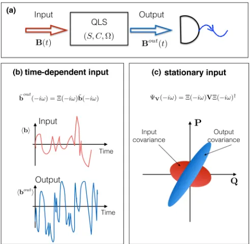
In a nutshell, system identification deals with the estimation of dynamical parameters of input-output systems from data obtained by performing measurements on the output fields. We distinguish two contrasting approaches to the identification of linear systems, which we illustrate in Fig. 1. In the first approach, one probes the system with a knowntime-dependent
input signal (e.g., coherent state), then uses the output measurement data to compute an estimator of the unknown dynamical parameter. In the Laplace domain, the input and output fields are related by a linear transformation given by the 2m×2mtransfer function(s):
˘
bout(s)=(s) ˘b(s), (1)
FIG. 1. (a) System identification problem: find parameters (S,C,) of a linear input-output system by measuring output. (b) Time-dependent scenario: in frequency domain, input and output are related by the transfer function (−iω) which depends on (S,C,). (c) Stationary scenario:power spectrumdescribes output covariance which is quadratic with respect to(−iω).
transfer function cannot be distinguished. Therefore, the basic identifiability problem is to find the equivalence classes of systems with the same transfer function.
In [17,46] this problem was analyzed for the special class ofpassivequantum linear systems (PQLSs) and it was shown thatminimalequivalent systems are related byn×nunitary
transformations acting on the space of annihilation modesa. By definition a QLS is minimal if no lower dimensional system has the same transfer function, which in the passive case is equivalent to the system being either observable, controllable, or Hurwitz stable [17]. In Sec.IIIwe answer the identifiability question for the case of general (not necessarily passive) QLSs; we show that the equivalence classes are determined by
symplectictransformations acting on the doubled-up space of canonical variables ˘a. It is worth noting that while in the clas-sical setup equivalent linear systems are related bysimilarity
transformations, in both quantum scenarios described above the transformations are more restrictive due to the unitary nature of the dynamics.
In the second approach, the input fields are prepared in a stationary in time, pure Gaussian state with independent increments (squeezed vacuum noise), which is completely characterized by the covariance matrixV =V(N,M) and the associated quantum Ito rule [16],
dB(t)dB(t)† dB(t)dB(t)T
dB#(t)dB(t)† dB#(t)dB(t)T
=
NT +1 M M† N
dt:=V dt.
If the system is minimal and Hurwitz stable, the dynamics exhibits an initial transience period after which it reaches stationarity and the output is in a stationary Gaussian state, whose covariance in the frequency domain is given by the
power spectrum
V(−iω)=(−iω)V (−iω)†.
Since the power spectrum depends quadratically on the transfer function, the parameters which are identifiable in the stationary scenario will also be identifiable in the time-dependent one. Our goal is to understand to what extent the converse is also true. First, we note that for a given minimal system there may exist lower dimensional systems with the same power spectrum. To understand this, consider the system’s stationary state and note that it can be uniquely written as a tensor product between a pure and a mixed Gaussian state (cf. the symplectic decomposition). In Theorem2we show that restricting the system to the mixed component leaves the power spectrum unchanged. Furthermore, the pure component is passive, which ties in with previous results of [23]. Conversely, if the stationary state is fully mixed, there exists no smaller dimensional system with the same power spectrum. Such systems will be calledglobally minimal, and can be seen as the analog of minimal systems for the stationary setting.
One of the main results is Theorem 3 which shows that for “generic” globally minimal single-input–single-output (SISO) systems which admit a cascade representation, the power spectrumV(s) determines the transfer function(s)
uniquely, and therefore the time-dependent and time-stationary identifiability problems are equivalent. It is interesting to note that this equivalence is a consequence of unitarity and purity of the input state, and does not hold for generic classical linear systems [38,41].
The paper is structured as follows. In Sec. IIwe review the setup of input-output QLSs, and their associated transfer function. We discuss in greater detail the two identifiability approaches mentioned above. In Sec. III we study the identifiability of QLSs in the time-dependent input setting. In Theorem 1 we show that the equivalence classes of input-output systems with the same transfer function are given by symplectic transformations of the system’s modes. We further show how a physical realization can be constructed from the system’s transfer function. In Sec.IVwe analyze the identifiability of QLSs in a stationary Gaussian noise input setting. We introduce the notion of global minimality for systems with minimal dimension for a given power spectrum, and show that a system is globally minimal if and only if it has a fully mixed stationary state, cf. Theorem2. In Sec.V
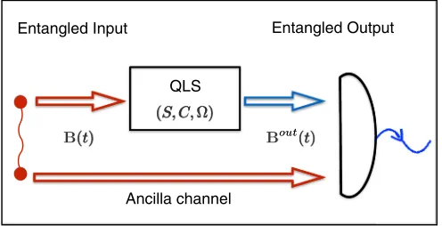
we analyze the structure of the power spectrum identifiability classes, and show that the power spectrum determines the transfer function uniquely, for a large class of SISO systems, cf. Theorem3. Finally, we show that using an additional input channel with an appropriately chosen entangled input ensures that the system is always globally minimal.
A. Preliminaries and notation
We use the following notations: “Tr” and “Det” denote the trace and determinant of a matrix, respectively. For a matrix X=(Xij) the symbolsX#=(Xij∗),X
T =(X
[image:2.608.49.295.69.309.2]represent the complex conjugation, transpose, and adjoint matrix respectively, where “*” indicates complex conjugation. We also use the doubled-up notation ˘X:=[XT,(X#)T]T and
(A,B) :=[A,B;B#,A#]. For example, we may write the transformationY =AX+BX# indoubled-upform as ˘Y = (A,B) ˘X. For a matrix Z∈R2n×2m define Z =J
mZ†Jn,
whereJn=[1n,0; 0,−1n]. Spec(X) is the set of all distinct
eigenvalues of X. A similar notation is used for matrices of operators. We use “1” to represent the identity matrix or operator. δj k is Kronecker δ and δ(t) is Dirac δ. The
commutator is denoted by [·,·].
Definition 1. A matrixS∈C2m×2mis said to beunitary
if it is invertible and satisfies
SS=SS=12m.
If additionally, S is of the formS=(S−,S+) for some S−,S+∈Rm×mthen we say that it issymplectic. Such matrices
form a group called thesymplectic group[16,48].
II. QUANTUM LINEAR SYSTEMS
In this section we briefly review the QLS theory, high-lighting along the way results that will be relevant for this paper. We refer to [26] for a more detailed discussion on the input-output formalism, and to the review papers [12,14,47,49] for the theory of linear systems.
A. Time-domain representation
A linear input-output quantum system is defined as a continuous variables (cv) system coupled to a Bosonic environ-ment, such that their joint evolution is linear in all canonical variables. The system is described by the column vector of annihilation operators,a:=[a1,a2, . . . ,an]T, representing the
ncv modes. Together with their respective creation operators a#:=[a#1,a#2, . . . ,a#n]
T
they satisfy the canonical commutation relations (CCRs) [ai,a∗j]=δij1.We denote byH:=L2(Rn)
the Hilbert space of the system carrying the standard repre-sentation of thenmodes. The environment is modelled bym bosonic fields, calledinput channels, whose fundamental vari-ables are the fieldsB(t) :=[B1(t),B2(t), . . . ,Bm(t)]T, where
t∈Rrepresents time. The fields satisfy the CCR
[Bi(t),B#j(s)]=min{t,s}δij1. (2)
Equivalently, this can be written as [bi(t),bj#(s)]=δ(t−
s)δij1, where bi(t) are the infinitesimal (white noise)
an-nihilation operators formally defined as bi(t) :=dBi(t)/dt
[14]. The operators can be defined in a standard fashion on the Fock space F =F(L2(R)⊗Cm) [4]. For most of the
paper we consider the scenario where the input is prepared in a pure, stationary in time, mean-zero, Gaussian state
with independent increments characterized by the covariance matrix
dB(t)dB(t)† dB(t)dB(t)T
dB#(t)dB(t)† dB#(t)dB(t)T
=
NT +1 M
M† N
dt
:=V(N,M)dt, (3)
where the brackets denote a quantum expectation. Note that N =N†,M=MT, andV 0, which ensures that the state
does not violate the uncertainty principle. The state’s purity can be characterized in terms of the symplectic eigenval-ues of V, as will be discussed in Sec. IV. In particular, N =M=0 corresponds to the vacuum state, while pure squeezed states for single-input–single-output (SISO) systems (i.e., m=1) satisfy |M|2=N(N+1). More generally, we
consider a nonstationary scenario where the input state has time-dependent meanB(t), e.g., a coherent state with time-dependent amplitude. For more details on Gaussian states see [50,51].
The dynamics of a general input-output system is deter-mined by the system’s Hamiltonian and its coupling to the environment. In the Markov approximation, the joint unitary evolution of system and environment is described by the (interaction picture) unitary U(t) on the joint space H⊗F, which is the solution of the quantum stochastic differential equation [4,26,47,49,52]
dU(t) :=U(t+dt)−U(t)
= −iHdt+LdB(t)†−L†dB(t)−12L†Ldt U(t), (4)
with initial condition U(0)=I. Here, H and L are system operators describing the system Hamiltonian and coupling to the fields; dBi(t),dB#i(t) are increments of fundamental
quantum stochastic processes describing the creation and annihilation operators in the input channels.
For the special case of linearsystems, the coupling and Hamiltonian operators are of the form
L=C−a+C+a#,
H=a†−a+12aT†+a+12a†+a#,
for m×n matrices C−,C+ and n×n matrices −,+ satisfying−=†−and+=T+.
As shown below, this ensures that all canonical variables evolve linearly in time. Indeed, let a(t) and Bout(t) be the
Heisenberg evolved system and output variables
a(t) :=U(t)†aU(t), Bout(t) :=U(t)†B(t)U(t). (5)
By using the QSDE (4) and the Ito rules (3) one can obtain the following Ito-form quantum stochastic differential equation of the QLS in the doubled-up notation [16]
da˘(t)=Aa˘(t)dt−CdB˘(t), (6)
dB˘out(t)=Ca˘(t)dt+dB˘(t), (7)
where a˘:=(aT,a#T)T, C:=(C
−,C+), and A:=
(A−,A+)= −12CC−iJnwith=(−,+) and
A∓:= −12(C−†C∓−C+TC±#)−i∓.
It is important to note that not all choices ofAandCmay be physically realizable as open quantum systems [15].
B. Controllability and observability
By taking the expectation with respect to the initial joint system state of Eqs. (6) we obtain the following classical linear system:
da˘(t) =Aa˘(t)dt−CdB˘(t), (8)
dB˘out(t) =Ca˘(t)dt+dB˘(t). (9)
Definition 2. The quantum linear system (6) is said to be Hurwitz stable (respectively controllable, observable) if the corresponding classical system (8) is Hurwitz stable (respectively controllable, observable).
In general, for a quantum linear system observability and controllability are equivalent [21]. A system possessing one (and hence both) of these properties is called minimal. Checking minimality comes down to verifying that the rank of the following observability matrix is 2n:
O=[CT,(CJn)T, . . . ,[C(Jn)2n−1]T]T,
where=(−,+). In the case of passive systems Hurwitz stability is further equivalent to minimality of the system [17,46]. However for active systems, although the statement [Hurwitz ⇒ minimal] is true [23], the converse statement ([minimal⇒Hurwitz]) is not necessarily so. We see this by means of a counterexample.
Example 1. Consider a general one-mode SISO QLS, which is parametrized by=(ω−,ω+) andC =(c−,c+). The system is Hurwitz stable (i.e., the eigenvalues ofAhave a strictly negative real part) if and only if
(1)|c−|>|c+|and|ω−||ω+|, or (2)|ω+|>|ω−|and|ω+|2− |ω
−|2< 12(|c−|2− |c+|2). A system is nonminimal if and only if the following matrix has rank less than 2:
C CJn
=
⎡ ⎢ ⎢ ⎢ ⎣
c− c+
c+# c
−#
c−ω−−c+ω+# c−ω+−c+ω−
c+#ω
−−c−#ω+# c+#ω+−c−#ω−
⎤ ⎥ ⎥ ⎥ ⎦.
Clearly it is possible for a system to be {minimal} ∩ {Hurwitz} or {nonminimal} ∩ {non-Hurwitz}. Further, for a counterexample to the statement [minimal ⇒ Hurwitz] consider for example|c+|>|c−|withω+=ω−.
In light of the previous example, we make the physical assumption that all systems considered throughout this paper are Hurwitz (hence minimal).
C. Frequency-domain representation
For linear systems it is often useful to switch from the time domain dynamics described above to the frequency domain picture. Recall that the Laplace transform of a generic process x(t) is defined by
x(s) :=L[x](s)= ∞
−∞
e−stx(t)dt, (10)
wheres∈C. In the Laplace domain the input and output fields are related as follows [8]:
˘
bout(s)=(s) ˘b(s), (11)
where(s) is thetransfer function matrixof the system
(s)= {1m−C(s1n−A)−1C} =
−(s) +(s)
+(s#)#
−(s#)#
.
(12) In particular, the frequency domain input-output relation is
˘
bout(−iω)=(−iω) ˘b(−iω).
The corresponding commutation relations are [b(−iω),b(−iω)#]=iδ(ω−ω)1, and similarly for the output modes [53]. As a consequence, the transfer matrix (−iω) is symplectic for all frequenciesω[16].
More generally one may allow for static scattering (imple-mented by passive optical components such as beamsplitters) or static squeezing processes to act on the interacting field before interacting with the system. The corresponding transfer function is obtained by multiplying the transfer function (12) with the scattering or squeezing symplectic matrixS on the right [16].
In the case of passive systems, +(s)≡0 and so the doubled-up notation is no longer necessary; the input-output relation becomes [8,46]
bout(s)=(s)b(s), (13)
where the transfer function is given by
(s)= {1m−C−(s1n−A−)−1C†−}S, (14)
which is unitary for alls= −iω∈iR. In the case of passive systems we write the triple determining the evolution as (S,C−,−), where the scattering matrixSis unitary.
Finally, we note that while the transfer function is uniquely determined by the triple (S,C,), the converse statement is not true, as discussed in detail in the next section.
III. TRANSFER FUNCTION IDENTIFIABILITY A. Identifiability classes
We now consider the following general question: which dynamical parameters of a QLS can be identified by observing the output fields for appropriately chosen input states? This is the quantum analog of the classical system identification problem addressed in [39–41]. The input-output relation (11) shows that the experimenter can at most identify the transfer function(s) of the system. Systems which have the same transfer function are calledequivalentand belong to the same
equivalence class.
Before answering this question for general QLSs we discuss the case of passive QLSs considered in [46]. The transfer function in Eq. (13) can be identified by sending a coherent input signal of a given frequencyωand known amplitudeα(ω), and measuring the output state, which is a coherent state of the same frequency and amplitude(−iω)α(ω).
that at frequencies far from the internal frequencies of the system, the input-output is dominated by the scattering and/or squeezing between the input fields. Our first main result is to extend this result to general (active) linear systems.
Theorem 1. Let (S,C,) and (S,C,) be two minimal and stable QLSs. Then they have the same transfer function if and only if there exists a symplectic matrixT such that
Jn=T JnT, C=CT S=S. (15)
Proof. First, using the same argument as above, the scat-tering and/or squeezing matricesSandSmust be equal.
It is known [32] that two minimal classical linear systems
dx(t)=Ax(t)dt+Bu(t)dt, dy(t)=Cx(t)dt+Du(t)dt
and
dx(t)=Ax(t)dt+Bu(t)dt, dy(t)=Cx(t)dt+Du(t)dt
for inputu(t), outputy(t), and system statex(t) have the same transfer function if and only if
A=T AT−1, B=T B, C=CT−1, D=D
for some invertible matrix T. Hence, for our setup C(s1−A)−1C =C(s1−A)−1Cif and only if there exists
an invertible matrixT such that
A=T AT−1, C=T C, C=CT−1.
Note that at this stage T is not assumed to be symplectic. The second and third conditions implyC=C(TT), which further implies that [TT ,CC]=0. Now by earlier definitions A= −12CC−iJ
n, so that the second and third conditions
applied to the first condition imply that Jn=T JnT−1.
Next, using this and the observation (Jn)=Jnit follows
that [TT ,Jn]=0.
Now,C(Jn)k=C(TT)(Jn)k=C(Jn)k(TT) which
means that the minimality matrix O satisfies O=OTT.
Because the system is minimal O must be full rank, hence TT =1.
Finally, it remains to show that the matrixT generating the equivalence class is of the form
T =
T1 T2
T#
2 T1#
.
To see this, observe thatCAk, CAk must be of the of this doubled-up form for k∈ {0,1,2, . . .}. Writing CAk, CAk,
andT as (P(k) Q(k) Q#
(k) P(#k)
), (P(k) Q(k) Q#
(k) P(k#)
) andT =(T1 T2
T3 T4), and using
the above result,CAk=CAkT, it follows that
P(k)T1†−T4T +Q(k)T3T −T2† =0
and
Q(k)# T1†−T4T +P(k)# T3T −T2† =0.
Hence
O
T1†−T4T
T3T −T2†
=0
and so using the fact thatO is full rank gives the required
result.
Therefore, without any additional information, we can at most identify the equivalence class of systems related by a symplectic transformation (on the system). Note that the above transformation of the system matrices is equivalent to a change of coordinates ˘a→Ta˘in Eq. (6).
B. Identification method
Suppose that we have constructed the transfer function from the input-output data, using for instance one of the techniques of [32] and [54].
Here we a outline a method to construct a system realization directly from the transfer function, for a general SISO quantum linear system. The realization is obtained indirectly by first finding a nonphysical realization and then constructing a physical one from this by applying a criterion developed in [21]. The construction follows similar lines to the method described in [17,46] for passive systems.
Let (A0,B0,C0) be a triple of doubled-up matrices which
constitute a minimal realization of(s), i.e.,
(s)=1+C0(sI−A0)−1B0. (16)
For example, in Appendix A such a realization is found for an n-mode minimal SISO system, with matrices (A,C), possessing 2n distinct poles each with a nonzero imaginary part. Any other realization of the transfer function can be generated via a similarity transformation
A=T A0T−1 B=T B0 C =C0T−1. (17)
The problem here is that in general these matrices may not describe a genuine quantum system in the sense that from a givenA,B,Cone cannot reconstruct the pair (,C). Our goal is to find a special transformationT mapping (A0,B0,C0) to a
triple (A,B,C) that does represent a genuine quantum system. Such triples are characterized by the following physical realizability conditions[21]:
A+A+CC=0 and B= −C. (18)
Therefore, substituting (17) into the left equation of (18) one finds
(T†J T)A0+A†0(T†J T)+C0†J C0=0, (19)
where the matricesJ here are of appropriate dimensions. Next, because the system is assumed to be stable it follows from [43, Lemma 3.18] that Eq. (19) is equivalent to
TT =J(T†J T)= ∞
0
J(C0eA0t)†J(C0eA0t)dt. (20)
We now need to use a result from [19], which is a sort of singular value decomposition for symplectic matrices. We state the result in a slightly different way here.
Lemma 1. LetN2n×2nbe a complex, invertible, doubled-up
matrix and letN =NN.
(1) Assume that all eigenvalues of N are semisimple [55]. Then there exists a symplectic matrix W such that N =WN Wˆ where ˆN =(Nˆ1 Nˆ2
ˆ N#
2 Nˆ1#
) with
ˆ
N1 =diag
λ+1, . . . ,λ+r
1,λ
−
1, . . . ,λ−r2,μ112, . . . ,μr312 ,
ˆ
N2 =diag
Hereλ+i >0,λ−i <0 andλci :=μi+iνi(withμi,νi ∈Rνi>0)
are the eigenvalues of N. The matrixσ =(0i −0i) is one of the Pauli matrices and12is the identity.
(2) There exists another symplectic matrix V such that N =VN W¯ where ¯N is the factorization of ˆN ( ˆN =N¯N¯) given by ¯N =(N¯1 N¯2
¯ N#
2 N¯1#
) with
¯
N1=diag
λ+1, . . . ,
λ+r1,0, . . . ,0,α112, . . . ,αr312
¯
N2=diag0, . . . ,0,
|λ−1|, . . . ,λ−r2,−β1σ, . . . ,−βr3σ .
The coefficientsαi andβi are determined fromμiandνi via
(i) Ifμi 0, thenαi= √μicoshxi,βi = √μisinhxi, with
xi =12sinh−1μν.
(ii) If μi 0, then αi = √
|μi|sinhxi,βi = √
|μi|coshxi,
withxi = 12sinh−1|μν|.
(iii) Ifμi =0, thenαi =βi =
νi 2.
The lemma can be extended beyond the semisimple assumption, but since the latter holds for generic matrices [19], it suffices for our purposes.
We can therefore use Lemma1 together with Eq. (20) in order to write the “physical” T as T =VT W¯ , where W
and ¯T can be computed as in the lemma above, and V is a symplectic matrix. However, since the QLS equivalence classes are characterized by symplectic transformation, this means thatT0=T W¯ transforms (A0,B0,C0) to the matrices
of a quantum systems satisfying the realizability conditions. Finally, we can solve to find the set of physical parameters (,C), which are given in terms of (A0,B0,C0), as
C=C0WT¯−1,
=iT W¯ A0WT¯−1+12
¯
T −1WC0C0WT¯−1 .
Remark 1. Note that, by assumption,(s) is the transfer function of a QLS. Since the original triple (A0,B0,C0)
is minimal, this implies that there exists a nonsingular T satisfying (20), so the right side of (20) is nonsingular, which eventually leads to a nonsingular transformationT computed using Lemma1.
Remark 2. The proof also holds for Multiple-input-multiple-output (MIMO) systems provided that one can find a minimal doubled-up (nonphysical) realization beforehand.
C. Cascade realization of QLS
Recently, a synthesis result has been established showing that the transfer function of a “generic” QLS has a pure cascade realization [18]. Translated to our setting, this means that given an-mode QLS (C,), one can construct an equivalent system (i.e., with the same transfer function) which is a series product of single mode systems. The result holds for a large class of systems characterized by the fact that the matrix A admits a certain symplectic Schur decomposition, which holds for a dense, open subset of the relevant set of matrices.
Assuming that such a cascade is possible, the transfer function is an n-mode product of single mode transfer
functions, which are given by
i(s)=
i−(s) i+(s)
i+(s#)# i−(s#)#
.
Further, we can stipulate that the coupling to the field is of the formC =(C−,0), with each element ofC− being real and positive. Indeed, since the system is assumed to be stable, there exists a local symplectic transformation on each mode so that coupling is purely passive. The point of this requirement is that it fixes all the parameters, so that under these restrictions each equivalence class from Sec.IIIcontains exactly one element. Note that the Hamiltonian may still have both active and passive parts. Therefore, each one mode system in the series product is characterized by three parameters,ci,i−∈Rwith
ci=0, and i+∈C. Ifi+=0 then the mode is passive.
Actually, it is more convenient for us here to reparametrize the coefficients so that
i−(s)=
s2−x2
i −yi2+2ixiθi
(s+xi+yi)(s+xi−yi)
,
i+(s)=
−2ixieiφi
y2
i +θi2
(s+xi+yi)(s+xi−yi)
,
where xi= 12c2i, yi=
|i+|2−2i−, θi=i−, and φi =
arg(i+). Therefore, from the properties of the individual
i±(s), one finds that−(s) and+(s) can be written as
−(s)=
n
i=1
(s−λi)(s+λi)
(s+xi+yi)(s+xi−yi)
, (21)
+(s)=γ
j
i=1(s−γi)(s+γi)
n
i=1(s+xi+yi)(s+xi−yi)
, (22)
withγ ,γi,λi ∈C,xi ∈R, andyieither real or imaginary, while
jis some number between 1 andn−1. In particular, the poles are either in real pairs or in complex-conjugate pairs.
Furthermore, there is a possibility that some of the poles and zeros may cancel in (21) and (22), and as a result some of these poles and zeros could be fictitious (see proof of Theorem3later where this becomes important).
For passive systems such a cascade realization is always possible [13,21] and each single mode system is passive. We show how this may be done in the following example.
Example 2. Consider a SISO PQLS (C,) and let z1,z2, . . . ,zmbe the eigenvalues ofA= −i−12C†C. Then
the transfer function is given by
(s)=Det(s−A
#)
Det(s−A)
=s−z#1
s−z1 ×
s−z# 2
s−z2 × · · · ×
s−z# 1
s−z1
.
Now, comparing each term in the product with the transfer function of a SISO system of one mode, i.e.,
(s)= s+i−
1 2|c|2
s+i+1
2|c|2
,
i = −Im(zi) and 1/2|ci|2= −Re(zi). This realization of the
transfer function is a cascade of optical cavities. Furthermore, we note that the order of the elements in the series product is irrelevant; in fact a differing order can be achieved by a change of basis on the system space (see Sec.III).
In actual fact this result enables us to find a system realization directly from the transfer function, thus offering a parallel strategy to the realization method in Sec.III Bfor passive systems. Note that a similar brute-force approach for finding a cascade realization of a general SISO system is also possible. However, the active case is more involved than the passive case, as the transfer function is characterized by two quantities, −(s) and +(s), rather than just one. For this reason and also that Sec.III Bindeed already offers a viable realization anyway, we do not discuss the result here.
IV. POWER SPECTRUM SYSTEM IDENTIFICATION Until now we addressed the system identification problem from atime-dependentinput perspective. We are now going to change viewpoint and consider a setting where the input fields arestationary(quantum noise) but may have a nontrivial covariance matrix (squeezing). In this case the characterization of the equivalence classes boils down to finding which systems have the same power spectrum, a problem which is well understood in the classical setting [41] but has not been addressed in the quantum domain.
The input state is “squeezed quantum noise,” i.e., a zero-mean, pure Gaussian state with time-independent increments, which is completely characterized by its covariance matrix V =V(M,N), cf. Eq. (3). In the frequency domain the state can be seen as a continuous tensor product over frequency modes of squeezed states with covarianceV(M,N). Since we deal with a linear system, the input-output map consists of applying a (frequency dependent) unitary Bogoliubov trans-formation whose linear symplectic action on the frequency modes is given by the transfer function
˘
bout(−iω)=(−iω) ˘b(−iω).
Consequently, the output state is a Gaussian state consisting of independent frequency modes with covariance matrix
b˘out(−iω) ˘bout(−iω)† =
V(−iω)δ(ω−ω),
where V(−iω) is the restriction to the imaginary axis of
thepower spectral density(or power spectrum) defined in the Laplace domain by
V(s)=(s)V (−s#)†. (23)
Our goal is to find which system parameters are identifiable in the stationary regime where the quantum input has a given covariance matrix V. Since in this case the output is uniquely defined by its power spectrumV(s) this reduces to
identifying the equivalence class of systems with a given power spectrum. Moreover, since the power spectrum depends on the system parameters via the transfer function, it is clear that one can identify “at most as much as” in the time-dependent setting discussed in Sec.III. In other words the corresponding equivalence classes are at least as large as those described by symplectic transformations (15).
In the analogous classical problem, the power spectrum can also be computed from the output correlations. The spectral factorization problem [42] is tasked with finding a transfer function from the power spectrum. There are known algorithms [42,44] to do this. From the latter, one then finds a system realization (i.e., matrices governing the system dynamics) for the given transfer function [32]. The problem is that the map from power spectrum to transfer functions is nonunique, and each factorization could lead to system realizations of differing dimension. For this reason, the concept ofglobal minimalitywas introduced in [39] to select the transfer function with smallest system dimension. This raises the following question: Is global minimality sufficient to uniquely identify the transfer function from the power spectrum? The answer is in general negative [56], as discussed in [38,41] (see also Lemma 2 and Corollary 1 in [45] for a nice review). Our aim is to address these questions in the quantum case. In the following section we define an analogous notion of global minimality, and characterize globally minimal systems in terms of their stationary state. Afterwards we show that for SISO systems which admit a cascade realization the power spectrum and transfer function identification problems are equivalent.
Global minimality
As discussed earlier, in the time-dependent setting it is meaningful to restrict the attention to minimal systems, as they provide the lowest dimensional realizations which are consistent with a given input-output behavior. In the stationary setting however, it may happen that a minimal system can have the same power spectrum as a lower dimensional system. For instance if the input is the vacuum and the system is passive then the stationary output is also vacuum and the power spectrum is trivial, i.e., the same as that of a zero-dimensional system. We therefore need to introduce a more restrictive minimality concept, as the stationary regime (power spectrum) counterpart of time-dependent (transfer function) minimality. The results of this section are valid for general MIMO systems and do not assume the existence of a cascade realisation.
Definition 3. A systemG=(S,C,) is said to beglobally minimal for input covariance V if there exists no lower dimensional system with the same power spectrum V. We
call (G,V) aglobally minimal pair.
Before stating the main result of this section we briefly review some symplectic diagonalization results which will be used in the proof. Consider ak-modes cv system with canonical coordinates ˘cand a zero-mean Gaussian state with covariance matrixV := c˘c˘†. Any change of canonical coordinates which preserves the commutation relations is of the form ˘c→c˘= Sc˘whereSis a symplectic transformationS, cf. Definition1. In the basis ˘c, the state has covariance matrix V=SV S†. In particular there exists a symplectic transformation such that the modescare independent of each other, and each of them is in a vacuum or a thermal state, i.e.,Vi:= c˘ic˘i† =(ni+1 0
0 ni)
where ni is the mean photon number. We call ˘ca canonical
basis, and the elements of the ordered sequencen1· · ·nk
thesymplectic eigenvaluesofV. The latter give information about the state’s purity: if allni=0 the state is pure, if all
ni >0 the state is fully mixed. More generally, we can separate
the pure and mixed modes and writec=(cTp,c T m)
T
This procedure can be applied to the m input modes b, with covariance V(N,M). Since the input is assumed to be pure, we haveSinV(N,M)Sin† =VvacwhereSinis a symplectic
transformation andVvacis the vacuum covariance matrix. The
interpretation is that any pure squeezed state looks like the vacuum when an appropriate symplectic “change of basis” is performed on the original modes.
Similarly, we can apply the above procedure to the stationary state of the system. Its covariance matrix P is the solution of the Lyapunov equation
AP +P A†+CV(C)†=0. (24)
By an appropriate symplectic transformation we can change to a canonical basis ˘a=Ssysa˘ such thataT =(aT
p,aTm). The
system matrices are nowA=SsysASsys ,C=CSsys . Note that
this transformation is of the form prescribed by Theorem 1, but the interpretation here is that we are dealing with the same system seen in a different basis, rather than a different system with the same transfer function.
By combining the two symplectic transformations we see that any linear system with pure input can be alternatively described as a system with vacuum input and a canonical basis of creation and annihilation operators.
The following theorem links global minimality with the purity of the stationary state of the system.
Theorem 2. Let G:=(S,C,) be a QLS with pure
squeezed input of covarianceV =V(M,N).
(1) The system is globally minimal if and only if the (Gaussian) stationary state with covariance P satisfying the Lyapunov equation (24) is fully mixed.
(2) A nonglobally minimal system is the series product of its restriction to the pure component and the mixed component. (3) The reduction to the mixed component is globally minimal and has the same power spectrum as the original system.
Proof. Let us prove the result first in the caseS=1. First, perform a change of system and field coordinates as described above, so that the input is in the vacuum state, while the system modes decompose into its “pure” and “mixed” parts aT =(aT
p,aTm). Note that this transformation will alter
the coupling and Hamiltonian matrices accordingly, but we still denote them andC to simplify notations. Therefore, in this basis the stationary state of the system is given by the covariance
P =
R+1 0
0 R
, R =
0 0
0 Rm
and satisfies the Lyapunov equation (24).
(⇒) We show that if the system has a pure component, then it is globally reducible. Let us writeA±andC±as block matrices according to the pure-mixed splitting,
A±=
App± Apm±
Amp± Amm±
, C±=(C±p,C±m),
so that the Lyapunov equation (24) can be seen as a system of 16 block matrix equations. Taking the (1,1) and (1,3) blocks, which correspond to theapa†pandapapcomponents of the
stationary state, one obtains
A−pp+App−†+C−p†C−p =0, (25)
AppT+ −C−p†C+p =0. (26)
SinceApp− = −ipp− −1/2(C−p†C−p−C+pTC+p#), Eq. (25) im-plies thatCpT+ C+p#=0, henceC+p =0. Therefore, using this fact in Eq. (26) givesApp+ =0, hencepp+ =0. These two tell us that the pure part contains only passive terms.
Consider now the (1,2) and (2,3) blocks, which correspond to theapa†mandamapcomponents of the stationary state.
From this, we get
Apm− (Rm+1)+A pm†
− +C−p†C−m=0, (27)
(Rm+1)A pmT
+ =0. (28)
Since Apm− +Apm− †+C−p†Cm
− =0, and Rm is invertible,
Eq. (27) implies Apm− =0. Similarly, Eq. (28) implies that Apm+ =0.
Let Gp:=(1,pp,Cp) be the system consisting of the
pure modes, withpp =(pp− ,0) andCp =(C−p,0). Let Gm
:=(1,mm,Cm) be the system consisting of the mixed modes withmm=(mm
− ,mm+ ) andCm=(C−m,C+m). We
can now show that the original system is the series product (concatenation) of the pure and mixed restrictions,
G=GmGp
.
Indeed, using the fact thatC+p =pp+ =Apm− =Apm+ =0, one can check that the series product has required matrices [9]
Cseries=C˜p+C˜m=C
and
series=˜pp+˜mm+Im
˜ CmC˜p
where the “tilde” notation stands for block matrices where only one block is nonzero, e.g., ˜Cp =(Cp,0), and Im
X:=
(X−X)/2i.
Now, let p,m(s) denote the transfer functions of Gp,m;
since the transfer function of a series product is the product of the transfer functions, we have (s)=m(s)·p(s). Furthermore, since Gp is passive and the input is vacuum,
we haveVp(s)=p(s)V p(−s#)†=V so that
V(s)=(s)V (−s#)†=m(s)V m(−s#)†
which means that the original system was globally reducible (not minimal).
together with the output at a long time 2T, and split the output into two blocks:A corresponding to an initial time interval [0,T] and B corresponding to [T ,2T]. If the system starts in a pure Gaussian state, then the S+A+B state is also pure. By ergodicity, at timeT the system’s state is close to the stationary state with symplectic rankdm. At this point the
system and output blockAare in a pure state so by appealing to the “Gaussian Schmidt decomposition” [57] we find that the state of the blockAhas the same symplectic eigenvalues (and rankdm) as that of the system. In the interval [T ,2T]
the outputAis only shifted without changing its state, but the correlations betweenAandSdecay. Therefore the jointS+A state is close to a product state and has symplectic rank 2dm.
On the other hand we can apply the Schmidt decomposition argument to the pure bipartite system consisting ofS+Aand Bto find that the symplectic rank ofBis 2dm. By ergodicity,
B is close to the stationary state in the limit of large times, which proves the assertion.
To extend the result toS=1, instead perform the change of field coordinatesV →SinSbV(SinSb)†at the beginning. The
proof for this case then follows as above because in this basis
S=1.
This result enables one to check global minimality by computing the symplectic eigenvalues of the stationary state. If all eigenvalues are nonzero, then the state is fully mixed and the system is globally minimal. We emphasize that the argument relies crucially on the fact that the input is a pure state. For mixed input states and in particular classical inputs, the stationary state may be fully mixed while the system is nonglobally minimal.
The next step is to find out which parameters of a globally minimal system can be identified from the power spectrum.
V. COMPARISON OF POWER SPECTRUM AND TRANSFER FUNCTION IDENTIFIABILITY
A. Power spectrum identifiability result
The main result of this section is the following theorem which shows that two globally minimal SISO systems have the same power spectrum if and only if they have the same transfer function, and in particular are related by a symplectic transformation as described in Theorem1.
Theorem 3. Let (C1,1) and (C2,2) be two globally
minimal SISO systems for fixed pure input with covariance V(N,M), which are assumed to be generic in the sense of [18]. Then
1(s)=2(s) for alls ⇔ 1(s)=2(s) for alls.
Proof. Recall that the power spectrum of a system (C,) is given by(s)V (−s#)†. Therefore, if
1(s)=2(s) then
1(s)=2(s). We will now prove the converse.
WritingV asS0(01 00)S†0 for some symplectic matrix S0,
we express the power spectrum as S0˜i(s)Vvac˜i(−s#)†S0†,
where ˜(s) is the transfer function of the system (1,S0C,) andVvacis the vacuum input. AsS0is assumed to be known,
the original problem reduces to proving the same statement for systems with vacuum input. In this case the power spectrum is
given by
−(s)−(−s#)# −(s)+(−s)
+(s#)#
−(−s#)# +(s#)#+(−s)
. (29)
The transfer function is completely characterized by the elements in the top row of its matrix, i.e.,−(s) and+(s). Also,−(s) and+(s) must be of the the form (21) and (22). Our first observation is that−(s) and+(s) in (21) and (22) cannot contain poles and zeros in the following arrangement: −(s) has a factor like
(s−λ#
i)(s+λ#i)
(s−λ#i)(s−λi)
=(s+λ#i)
(s−λi)
(30)
and+(s) contains a factor like
(s−λi)(s+λi)
(s−λ#
i)(s−λi)
= (s+λi)
(s−λ# i)
. (31)
For if this were the case and assuming that this could be done k times, then our original system could be decomposed as a cascade (series product) of two systems.
(i) The first system is ak-mode passive system with transfer function
(1)(s)=
(1)−(s) 0
0 (1)−(s#)#
, (32)
where
(1)−(s)=
k
i=1
(s+λ# i)
(s−λi)
, (1)−(s#)#=
k
i=1
(s+λi)
(s−λ# i)
.
Note that by Example2it is physical.
(ii) The second system has n−k modes and transfer function
(2)(s)=
(2)−(s) (2)+(s)
(2)+(s#)# (2)
−(s#)#
, (33)
where
(2)−(s)=−(s)
k
i=1
(s+μ# i)
(s−μi)
,
(2)+(s)=+(s)
k
i=1
(s+μi)
(s−μ# i)
.
It can be shown that there exists a minimal physical quantum system with this transfer function (see AppendixB).
Since(1)(s) is passive,
(1)(s)Vvac(1)(−s#)†=Vvac
and hence thisk-mode system is not visible from the power spectrum, while the power spectrum is the same as that of the lower dimensional system (2)(s). Therefore we have a
contradiction to global minimality.
of−(s) and+(s) from the three quantities:
−(s)−(−s#)#, (34)
−(s)+(−s), (35)
+(s#)#+(−s). (36)
First, all poles of−(s) and+(s) may be identified from the power spectrum. Indeed, due to stability, each pole in (34)–(36) can be assigned unambiguously to either−(s) or +(−s). However, cancellations between zeros and poles of the two terms in the product may lead to some transfer function poles not being identifiable, so we need to show that this is not possible. Suppose that a poleλof −(s) is not visible from the power spectrum. This implies the following:
(i) from (34),λis a zero of−(−s#)#[equivalently−λ#is
a zero of−(s)], and
(ii) from (35),λis a zero of+(−s) [equivalently−λis a zero of+(s)].
We consider two separate cases: λnonreal or real. Ifλis nonreal then from the symmetries of the poles and zeros in (21) and (22),−(s) will contain a term like
(s−λ#)(s+λ#) (s−λ#)(s−λ) =
(s+λ#)
(s−λ) (37)
and+(s) will contain a term like
(s−λ)(s+λ) (s−λ#)(s−λ) =
(s+λ)
(s−λ#). (38)
By the argument above, the system is nonglobally minimal as there will be a mode of the system that is nonvisible in the power spectrum. Therefore all nonreal poles of−(s) may be identified.
A similar argument ensures that all poles of +(s) are visible in the power spectrum.
Ifλis real, we show that−(s) and+(s) will have terms of the form (37) and (38) and the result will follow. Indeed sinceλis a pole of−(s), the denominator of (21) must have a second root atλsince the first cancels with the term (s−λ) which comes together with (s+λ) in the numerator. But then, +(s) must also have a pole atλsince otherwise|−(−iω)|2− |+(−iω)|2 =1 could not hold. A similar argument holds for a real pole of+.
Therefore we conclude that all poles of±(s) can be identi-fied from the power spectrum, and we focus next on the zeros. Unlike the case of poles, it is not clear whether a given zero in any of these plots belongs to the factor on the left or the factor on the right in each of these equation [i.e., to−(s) or −(−s#)#in (34), etc.].
Since the poles of−(s) and+(s) may be different due to cancellations in (21) and (22), it is convenient here to add in “fictitious” zeros into the plots (34)–(36) so that−(s) and +(s) have the same poles. Note that these fictitious poles and zeros would have been present in (21) and (22) before simpli-fication. From this point onwards, the zeros in (34)–(36) will refer to this augmented list which includes the additional zeros.
Real zeros. In general the real zeros of−(s) and+(s) come in pairs±λ[see Eqs. (21) and (22)], unless a pole and zero (or more than one) cancel on the negative real line. Our
task here is to distinguish these two cases from plots (34)–(36). −(s) has either (i) zeros at±λ, or (ii) a zero atλ >0 but not at−λ.
In case (i) (34) will have a double zero at each±λ, whereas in case (ii) (34) will have a single zero at±λ. We need to be careful here in discriminating cases (i) and (ii) on the basis of the zeros of (34). For example, a double zero atλin (34) could be a result of one case (i) or two cases (ii) in−(s). More generally, we could have annth order zero atλand as a result even more degeneracy is possible. A similar problem arises for the zeros of+(s) in (36).
Our first observation here is that it is not possible for both −(s) and+(s) to have zeros at±λ(takingλ >0 without loss of generality). If this were possible then by using the sym-plectic condition|−(−iω)|2− |
+(−iω)|2 =1 and the fact
that we are assuming that −(s) and +(s) have the same poles tells us that−(s) and+(s) must both have had double poles at−λ. The upshot is that−(s) and +(s) will have terms of the form (30) and (31), which is a contradiction.
Now, suppose (34) has nzeros at λ >0 and (36) has m zeros atλ >0. Then we know that−(s) must haven−2p zeros at−λandn+2p zeros atλ. Also,+(s) must have m−2q zeros at−λ and m+2q zeros at λ. The goal here is to findpandq because if these are known then it is clear that there must be
n−p
2 (
m−q
2 ) type (i) zeros andp (q) type (ii) zeros in −(s)
[+(s)].
By the observation above it is clear that either p=n or q =m. Also, in (35) there will be n+m+2p−q zeros atλ and
n+m+q−p
2 zeros at −λ. Hence q−p is known at this stage.
Finally, it is fairly easy to convince ourselves that if p=n but one concludes thatq =m(or vice versa) and using the value ofq−pleads to a contradiction. Hencepandqcan be determined uniquely. For example, ifn=2,m=5,q =2, and p=3 so thatq =nandq−p= −1. Then assuming wrongly thatp=5 and usingq−p= −1 it follows thatq =4 and so nmust be 6, which is incorrect.
Having successfully identified all real zeros, we now show how to identify the zeros of−(s) and+(s) away from the real axis.
Complex (nonreal) zeros.Comparing the zeros of (34) with those of (35) we find two cases in which the zeros can be assigned directly.
(i) Case 1: Letzbe a zero of (34) that is not a zero of (35). Thenzmust be a zero of−(−s#)#. Hence−z# is a zero of
−(s).
(ii) Case 2: Letwbe a zero of (35) that is not a zero of (34). Thenwmust be a zero of+(−s)#. Hence−wis a zero of +(s).
The question now is whether this procedure enables one to identify all zeros. Suppose that there is a zero v that is common to both of these plots. Then−v#must also be a zero
of (34). Now, if−v#is not a zero of (35) thenvis identifiable as belonging to−(s).
Therefore we can restrict our attention to the case that the zero pair {v,−v#}is common to both plots. Note that
in this instance the list of zeros of (36) will also contain