DOI 10.1007/s00466-016-1360-5 O R I G I NA L PA P E R
Stokes–Brinkman formulation for prediction of void formation
in dual-scale fibrous reinforcements: a BEM/DR-BEM simulation
Iván David Patiño1 · Henry Power2 · César Nieto-Londoño3 · Whady Felipe Flórez4
Received: 29 August 2016 / Accepted: 22 November 2016
© The Author(s) 2017. This article is published with open access at Springerlink.com
Abstract A numerical study of voids formation in
dual-scale fibrous reinforcements is presented. Flow fields in channels (Stokes) and tows (Brinkman) are solved via direct Boundary Element Method and Dual Reciprocity Boundary Element Method, respectively. The present approach uses only boundary discretization and Dual Reciprocity domain interpolation, which is advantageous in this type of moving boundary problems and leads to an accurate representation of the moving interfaces. A problem admitting analytical solu-tion, previously solved by domain-meshing techniques, is used to assess the accuracy of the present approach, obtaining satisfactory results. Fillings of Representative Unitary Cells at constant pressure are considered to analyze the influence of
B
Henry Powerhenry.power@nottingham.ac.uk Iván David Patiño
ivandavidpatino@gmail.com César Nieto-Londoño cesar.nieto@upb.edu.co Whady Felipe Flórez whady.florez@upb.edu.co
1 Grupo de Investigación en Nuevos Materiales (GINUMA), Universidad Pontificia Bolivariana, Circular 1 Avenida 73-76, Bloque 22B, Piso 1, Medellín, Colombia
2 School of Mechanical, Materials and Manufacturing Engineering, University of Nottingham, Coates Building, University Park, Nottingham NG7 2DR, UK
3 Grupo de Ingeniería Aeroespacial, Universidad Pontificia Bolivariana, Circular 1ra No 73-34 (Bloque 22), Medellín, Colombia
4 Grupo de Energía y Termodinámica, Universidad Pontificia Bolivariana, Circular 1ra No 73-34 (Bloque 22), Medellín, Colombia
capillary ratio, jump stress coefficient and two formulations (Stokes–Brinkman and Stokes–Darcy) on the filling process, void formation and void characterization. Filling times, fluid front shapes, void size and shape, time and space evolution of the saturation, are influenced by these parameters, but voids location is not.
Keywords Boundary Element Method·Stokes–Brinkman
formulation·Stress matching conditions·Void formation· Dual-scale fibrous reinforcement
1 Introduction
In dual-scale fibrous reinforcements used in composites pro-cessing, the permeability of the tows is several orders of magnitudes lower than the permeability of the inter-tow chan-nels. This causes imbalances between the flow inside the tows and the flow in the channels, which can lead to the formation of voids by mechanical entrapment of air. Once these voids are formed, several phenomena can take place, among others: bubble compression, displacement, migration and splitting.
Considering the shearing effect between the fluid and the walls of the porous medium, Brinkman (1947) added the second-order derivatives of the velocity to the Darcy equation, resulting in the Brinkman equation. The averages implicit in the Brinkman equation can be viewed as averages over an ensemble of different scales of the porous medium that interpolate between the Stokes and Darcy equations. On small length scales, the pressure gradient balances the Laplacian of the velocity and the flow is essentially viscous, Stokes flow, while over larger length scales, the velocity is slowly varying and the pressure gradient balances the aver-age velocity as it does in Darcy’s law (for more details see Durlofsky and Brady [9]). According to Ochoa-Tapia and Whitaker [40], Brinkman approximation can be applied when the following three length scale constrains are simultaneously satisfied:r02/
lεlp
1 ,r02/ (lεlv)1,lf r0, where lε, lp, lv andlf are the characteristic lengths associated
to the porosity, pressure, velocity gradients and fluid phase, respectively, andr0is the characteristic length scale of the Representative Elementary Volume (REV). Krotkiewski et al.[28] reported a direct numerical simulation of the flow field in homogeneous two dimensional porous media with characteristic lengthL and permeabilityK, concluding that the Stokes solution is dominant forK/L2≥10, Darcy law is representative of the flow field ifK/L2≤10−4, while for 10−4≤K/L2≤10 the Brinkman approximation should be used to account for the transition between both flow regimes, Stokes and Darcy.
The Brinkman equation includes an effective viscosity term,μe f f, to consider the viscous diffusion not deemed in
the Darcy law. In order to explain the meaning of this term, it is necessary to consider that the volume averaging method allows describing the porous medium flow in terms of aver-ages of the local quantities by means of the Darcy–Brinkman equation, which is given by (3) consideringμe f f =μ, where μis the real fluid viscosity. This last equality is valid pro-vided that a non-slip condition on the interfaces between the fluid and solid phases of the porous medium is consid-ered, as done in the traditional volume-averaging method. However, the non-coincidence betweenμe f f andμhas been
demonstrated in several experimental, numerical and theo-retical works, suggesting that the non-slip condition is not necessarily valid in all cases. For instance, Givler and Alto-belli [17] experimentally found thatμe f f is 7.5 times the
value ofμfor high-porous open cell foams and moderate Reynolds numbers, whereas Starov and Zhdanov [70] stud-ied the dependency ofμe f fon the porosity and particle size in
porous media composed of equally sized spherical particles, finding thatμe f f can be lower or larger thanμ. On the other
hand, the numerical flow simulations conducted by [4] in 3D regular arrays of cubes showed thatμe f f < μ, whereas those
ones executed by [34] indicated thatμe f f > μin order to
match the Brinkman equation with the numerical solutions in
the boundary layer developed in the porous medium domain when it is in contact with a free-fluid domain. A very illus-trative theoretical work was published by [63], where it was demonstrated that the effective viscosity, μe f f, is different
to the fluid viscosity,μ, when a slip condition at the fluid-solid interface of the porous medium is considered. Using an up-scaling procedure, a boundary-value problem to com-puteμe f f was obtained in such work, achieving important
conclusions. In general, the effective viscosity is different to the fluid viscosity, i.e, μe f f = μ, because it is a term
that ‘absorbs’ the microscale variations of the velocity gra-dient when a variationless velocity gragra-dient model is used at macroscopic scale. On the other hand, as the prescribed slip coefficient at the fluid-solid interface increases, the bound-ary layer thickness decreases and a non-slip condition tends to be reached, in such a way that in the limit when the slip coefficient tends to infinity,μe f f =μ.
In the Stokes–Brinkman approach the matching condi-tions at the interface channels-tows are defined in terms of the corresponding surface velocity and traction vectors. Con-tinuity of the velocity field is always considered and two types of conditions could be employed for the tractions: continu-ous [39] and jump stress [40,41]. The continuity of stress was initially implemented in [39,48], however a jump stress matching condition was proposed later in [40] based on the non-local form of the volume-averaged momentum equa-tion for the analysis of the region between the channel and the porous medium. By means of experiments of unidirec-tional flow in parallel domains, Ochoa-Tapia and Whitaker [41] found that the jump stress tensor across the interface for isotropic porous media, σi jnˆj, is linearly
propor-tional to the interface surface velocity uj, i.e.σi jnj = μTi juj/
√
K, whereμstands for the fluid viscosity, while the second-order tensorTi j is given byβδi j, withβas the jump
stress coefficient ranging between −1 and 1.47; for more details see [23]. However, Angot [2], demonstrated mathe-matically that the well-posedness of the Stokes–Brinkman problem is only possible whenβ ≥ 0. The theoretical esti-mation of the value ofβ was developed in [64,65], where it was established thatβdepends on the porosity of the porous medium in the inter-region channel-tow,εct.
The estimation of the effective viscosity term,μe f f, in
the Brinkman equation is known to depend on the geome-try of the porous medium and the flow itself. As suggested in the literature [23,56,57], an acceptable approximation for
μe f f in dual-scale fibrous reinforcements is to consider that μe f f = μ when the continuous stress condition is used,
whereasμe f f =μ/εt is suitable when the jump stress
con-dition is employed, withεt as the tow porosity. In a recent
has a strong influence on the boundary layer thickness in the porous medium, but not on the effective saturated permeabil-ity, which is dependent on the pore geometry. In this point, it is relevant to mention that the study of the pore geometrical dependency of the effective permeability could be a com-plicated and computational expensive task, but some recent efforts have been addressed to reduce the computational cost without compromising the accuracy. For instance, a mul-tiscale framework relating the effective permeability with some microstructural attributes extracted by X-ray tomog-raphy was proposed in [55], where several computational techniques were efficiently combined (Level Set, Graph The-ory and Lattice Boltzman/Finite Element) to determine the tortuosity, porosity and homogenized effective permeability at specimen scale. The particular problem solved in [23] by FEM is also considered here for validation of the numerical technique implemented.
In the present work, simulations of fillings of RUC’s (Representative Unitary Cells) of dual-scale fibrous rein-forcements are carried out using a Boundary Element/Dual Reciprocity numerical approach (BEM/DR-BEM). The flow in the channel, Stokes flow, is given by its boundary-only inte-gral formulation, Green’s formula, and numerically treated by direct BEM, while the flow inside the tows, Brinkman flow, is given by a boundary-domain integral formulation in terms of the Stokes fundamental solutions, where the domain integral is transformed into a boundary integral using the Dual Reciprocity Boundary Element Method (DR-BEM). The present numerical approach is validated by compari-son with a benchmark analytical solution used previously in the literature to assess the robustness of FEM-based numer-ical solutions of flow problems in dual-scale porous media [23,58].
The developed BEM/DR-BEM numerical scheme is then used to simulate the simultaneous filling of channels and tows inside the RUC at constant pressure regime with the purpose of analyzing the influence of the stress matching conditions on the void formation at several values of the capillary ratio,Ccap = Pcap,max/Pi n, where Pcap,max and Pi n stand for the maximum capillary pressure and the inlet
pressure, respectively. This type of filling problem has been previously considered in the literature using different formu-lations and numerical techniques. For instance, Gourichon et al. [19] studied the influence of the RUC porosity in the formation of voids using a Darcy–Darcy formulation and the FEM/CV conforming method. On the other hand, Schell et al. [49] studied the influence of the tow porosity,
εt, on the final void content using the same formulation and
numerical technique as in [19], while the problem of unidi-rectional filling of circular tows in cylindrical coordinates was analyzed in [68] using a Stokes–Brinkman formula-tion and the Finite Volume method, where it was studied the effect of the filling velocity, resin viscosity, inter-tow
dimension and intra-tow dimension on the shape of the fluid front.
In comparison with domain-meshing numerical tech-niques previously used in the literature for the simulation of the filling process in dual scale fibrous reinforcements based on the Stokes–Brinkman formulation [11,23,50,51,58], two main advantages can be identified by the use of the BEM/DR-BEM approach employed in this work. Firstly, the use of BEM-based techniques does not imply any mesh discretiza-tion of the problem domain, which is not a trivial task in a domain that is continuously changing in size and shape as in the present case. Secondly, the tracking of the fluid front is directly carried out by an Euler integration of the kinematic condition at the moving interface, which assures a higher order accuracy on the prediction of the fluid front shape with-out the need of implementing any additional reconstruction algorithm of the moving boundaries, contrary to the case of the Volume of Fluid (VOF) [14,15] or the Level Set Method [12,13,53].
Another important contribution of this work is the study of the influence of two types of stress matching conditions (con-tinuous and jump) on the void formation. Other works have analyzed the influence of these conditions on the effective saturated permeability [23,58], but not on the size, shape and location of the voids formed by mechanical entrapment of air. Additionally, the processes of the void formation using the Stokes–Brinkman and Stokes–Darcy formulations are com-pared each other, which has not been reported before to the best of our knowledge. Finally, the consideration of a flow direction-dependent capillary pressure in the tows without experimental factors and of the curvature- dependent surface traction effects for the fluid fronts in the channels are ones of the main differences between the present work and previous publications in the same field [1,7,49,59].
2 Governing equations, boundary and matching
conditions
In the Stokes–Brinkman formulation, the governing equa-tions at each medium are defined as:
Mass conservation (For all domains):
∂ui ∂xi =
0 (1)
Momentum for the Stokes domain (Channels flow):
μ ∂2ui ∂xjxj
− ∂p
∂xi =
0 (2)
μe f f ∂
2u
i ∂xj∂xj −
∂p ∂xi =
μ Ki
ui (3)
where in the right hand side of (3) the double index nota-tion is not considered fori =1,2. Hereui, p,μ,μe f f and Ki represent the velocity vector, pressure, liquid viscosity,
effective viscosity and main permeabilities, respectively. Let us define the following non-dimensional variables for the length, velocity, time and pressure [46,47]:
For all domains:
xi =xi/L∗ (4)
ˆ
ui =ui/Umax (5)
ˆ
t =t/L∗/Umax
(6)
For the Stokes domain (Channels flow):
ˆ
p= p
μ·Umax/L∗
(7)
For the Brinkman domain (Porous media or tows flow):
ˆ
p= p
μe f f ·Umax/L∗
(8)
whereL∗andUmaxare the characteristic length and the
max-imum velocity of the problem, respectively. In terms of these characteristic values, the non-dimensional form of the gov-erning Eqs. (1), (2), (3) can be written as:
∂uˆi ∂xˆi =
0 (9)
∂2uˆ
i ∂xˆjxˆj −
∂pˆ
∂xˆi =
0 (10)
∂2uˆ
i ∂xˆj∂xˆj −
∂pˆ
∂xˆi =χ
2
iuˆi (11)
whereχi2 =1/Dai∗ =(L∗)2μ/Ki.μe f f
is the inverse of the Darcian number,Dai∗, in the principal directioni.
The non-dimensional matching conditions for the Stokes– Brinkman problem are as follows [2]:
• Continuity of velocities:
ˆ
u(is)= ˆu(ib) (12)
• Normal and tangential component of the jump stress:
ˆ
ti(s)+μe f f/μ
ˆ
ti(b)
ˆ
ni = − L∗
√
Kn
βnuˆ(is)nˆi (13)
ˆ
ti(s)+μe f f/μ
ˆ
ti(b)
ˆ
τi = − L∗
√
Kτβτuˆ (s)
i τˆi (14)
wheres andbrepresent the Stokes and Brinkman domain, respectively, and tˆi(s) = (L∗/ (μUmax)) σi jnj and tˆi(b) =
L∗/μe f fUmax
σi jnj are defined as the dimensionless
traction vectors, withσi j as the Cauchy stress tensor. Here KnandKτ are the effective permeabilities in the normal and
tangential direction, respectively, with the effective perme-ability in any orientation,φi, given by [33]:
Ke f f(φi)=
K1·K2
K1·sin2(φi)+K2·cos2(φi)
(15)
whereφi is the angle between a given direction and the major
axis of permeability. In the above jump stress conditions,βn
andβτare the normal and tangential jump coefficients, which are considered equal in the present work as done in [23,58]. Some authors consider that the minus sign of the right hand side of (13) and (14) is implicit in the stress jump coefficients,
βnandβτ[23,58]. When a continuous surface traction at the
interface is considered, the corresponding matching condi-tion can be obtained from (13) and (14) by setting the values ofβnandβτ to zero.
In the present paper, the RUC filling is carried out at constant inlet pressure for all cases. Therefore, the non-dimensional inlet boundary conditions are as follows: At the Stokes domain:
ˆ
t1(s)= − ¯pL∗/ (μUmax)n1(s),uˆ(2s)=0 (16)
At the Brinkman domain:
ˆ
t1(b)= − ¯pL∗/μe f fUmax
n(1b),uˆ(2b)=0 (17)
wherep¯represents the prescribed inlet pressure. No-flux con-dition,uˆinˆi =0,and zero traction in the tangential direction,
ˆ
tiτˆi =0, are used in boundaries where symmetry is specified.
At the fluid fronts, kinematic and dynamic boundary con-ditions are defined. The former condition establishes that the fluid front advances along its normal direction, while the dynamic condition accounts for the discontinuities of normal stress due to the capillary pressure, pcap. Both kind of
con-ditions are represented in (18) and (19), (20), respectively:
• Kinematic condition (For all domains):
dxˆi/dtˆ= ˆunni =
ˆ
uj.nj
ni (18)
• Dynamic condition (At the Stokes domain):
ˆ
ti(s) =L∗pcap−pa
/ (μUmax)ni (19)
• Dynamic condition (At the Brinkman domain):
ˆ
ti(b)=L∗pcap−pa
/μe f fUmax
where ni, pa and uˆn are the outwardly oriented normal
vector, air pressure and dimensionless normal velocity at the fluid front, respectively. In (18),uˆn is given by the Stokes
velocity in the channel domain and by the pore velocity in the porous medium, which, in turn, is defined as the Brinkman velocity divided by the tow porosity,εt [32,67]. In the case
of the channel flow, the capillary pressure ispcap = −σ κ =
−σ∂nˆi/∂xi
, withσ as the surface tension and κ as the curvature of the moving boundary. For the flow inside the porous medium, the capillary pressure can be computed using the following equation [35]:
pcap =2(σ·cos(θ) /Rec) (21)
Rec =2
Ai nt,s/Ci nt,s
(εt/ (1−εt)) (22)
whereAi nt,sis the cross sectional area of the solid particles in
the flow direction,Ci nt,s is the wetted perimeter of the solid
particles,θis the contact angle andεt is the tow porosity. In
this work, the geometry of the porous medium is considered as a bank of aligned circular fibers and the capillary pressure in any point of the longitudinal tow (warp) depends on the angle between the normal of the fluid front and the principal axis of the fibers,ϕ. If the flow infiltrates the warp in parallel,
ϕ=0, or oblique direction, 0< ϕ < π/2, Ai nt,s andCi nt,s
are approximated as the cross sectional area and perimeter of a truncated circular cylinder using Gauss-Kummer series for the perimeter of the resulting ellipse [5], as given by:
Ai nt,s =nfπR2sec(ϕ) (23) Ci nt,s =nfπR(1+sec(ϕ))
×
1+ ∞
i=1
1/2
i
2
sec(ϕ)−1 sec(ϕ)+1
2i
(24)
If the impregnation occurs perpendicular to the fibers,ϕ =
π/2, the following equations are used:
Ai nt,s =2nfLfR (25)
Ci nt,s ≈2nfLf (26)
On the other hand, for the transverse tow (weft), it is accepted that the fluid front moves inward perpendicular to the fibers and it is used the mean capillary pressure given in [38] considering an hexagonal array of fibers:
pcap,r =(σ/R) .
sinαsup+θ
−sinαi n f +θ
5π
6 (1+η)−1− √
3/2
(27)
η=d/R=
π/2√3(1−εt)
−1 (28)
αsup ∼=(π/2−θ) (29)
αi n f ∼=(θ−π/2) (30)
whereR anddare the fiber radius and half-distance between fibers, respectively. The model of Gebart [16] for a hexagonal array is used to calculate the permeabilities in the principal directions:
K1=8R2·
1−Vf
3
c·Vf
2
(31)
K2=c1
Vf,max/Vf −1
5/2
R2 (32)
where Vf = 1 −εt is the fiber volume fraction, while
the parametersc,c1andVf,max are given by the following
expressions:
c=53 (33)
c1=16/(9π √
6) (34)
Vf,max =π/(2
√
3) (35)
3 Integral equation formulations and numerical
techniques
The Stokes–Brinkman problem of this work is solved using direct BEM and DR-BEM for the channel and tows domains, respectively, with the corresponding matching and boundary conditions presented in Section2. The integral formulation for the Stokes equation is the following:
ci j(ξ)uj(ξ)=
S
Ki j(s)(ξ,y)uj(y)d Sy
−
S
Uij(s)(ξ,y)tj(y)d Sy (36)
where ci j = (α/2π) δi j, with α as the solid angle in the
source point, whose value is α = π for points located over a smooth contour. For points located inside the domain,
ci j =δi j. In (36),uj andtj are the velocities and tractions
in the field points, respectively.
The fundamental solutions of the integral kernels of (36) are given by:
Uij(s)(ξ,y)= − 1
4π
ln
1
r
δi j+(ξ
i−yi)
ξj−yj
r2
(37)
Ki j(s)(ξ,y)= −1 π
(ξi−yi)ξj−yj(ξk−yk)nk(y)
r4 (38)
r= |ξ−y| (39)
the real space in the anisotropic case is not a trivial problem and to avoid these difficulties, a boundary-domain integral formulation in terms of the Stokes fundamental solutions is considered for the Brinkman equation and the resulting domain integral is transformed into a boundary integral using DR-BEM [42]. The integral formulation is as follows:
ci j(ξ)uj(ξ)=
S
Ki j(ξ,y)uj(y)d Sy
−
S
Uij(ξ,y)tj(y)d Sy
+
Uij(ξ,y)gj(y)dy (40)
In DR-BEM, the non-homogeneous term, gj(y) = χ2
juj(y), is approximated using Radial Basis Function
(RBF) interpolation given by Augmented Thin Plate Splines (ATPS). The augmented part of a generalized thin plate spline of ordernis a polynomial of ordern−1 that is added to obtain an invertible interpolation matrix [18]. In the present work,
n=2 and the form of the ATPS is as follows:
fm(y)=r2ln(r) f or m=1...,NB+NL (41) fm(y)=1 f or m=NB+NL+1 (42) fm(y)=y1 f or m=NB+NL+2 (43)
fm(y)=y2 f or m=NB+NL+3 (44)
where NB is the number of boundary points, NL is the
number of interior points andr(y,zm) = |y−zm| is the
distance between the field points,y, and the trial points,zm. Accordingly, the non-homogeneous term can be expanded as follows:
gj(y)=
NB+NL+3
m=1 αm
l δjlfm(y) , j=1,2; l =1,2
(45)
where αml represent the approximation coefficients in the directionl. The ATPS represented in (41) to (44) requires the addition of orthogonality conditions, as shown in the fol-lowing equation:
NB+NL
m=1 αm
l =
NB+NL
m=1 αm
l y m
1 =
NB+NL
m=1 αm
l y m
2 =0 (46)
After substituting (45) into (40), the integral representa-tion takes the following form:
ci j(ξ)uj(ξ)=
S
Ki j(ξ,y)uj(y)d Sy
−
S
Uij(ξ,y)tj(y)d Sy
+
NB+NL+3
m=1 αm
l
Uij(ξ,y) δjlfm(y)dy
(47)
The transformation of the domain integral into a boundary integral is accomplished by defining the following auxiliary Stokes field:
∂uˆ(jml)
∂yj =
0 (48)
μ∂ 2uˆ(ml)
j ∂yk∂yk −
∂pˆ(ml)
∂yj =
fm(y) δjl (49)
with the particular solutions for the ATPS given in [10]. The substitution of the auxiliary field defined in (48) and (49) into (47) and the application of the Green’s identities in the domain integral, lead to the following boundary-only integral representation:
ci j(ξ)uj(ξ)=
S
Ki j(ξ,y)uj(y)d Sy
−
S
Uij(ξ,y)tj(y)d Sy
+
NB+NL+3
m=1 αm
l (ci j(ξ)uˆ(jml)(ξ)
−
S
Ki j(ξ,y)uˆ(jml)(y)d Sy
+
S
Uij(ξ,y)tˆ(jml)(y)d Sy) (50)
where the coefficientsαlm are given in terms of the inverse of the interpolating matrix obtained by collocation of (45) at
NBboundary nodes and NL internal nodes.
The singularities arising in the kernels Ki j andUij of
(36) and (50) are dealt with the rigid body motion prin-ciple [45] and the Telles transformation [61], respectively. In these equations, the boundary and the physical variables are discretized using quadratic isoparametric interpolation. Additionally, discontinuous shape functions with a colloca-tion factor ofαdi s =2/3 are employed at the corners of the
and variables and the assembly of the resultant matrices, by considering the corresponding boundary and matching con-ditions, a linear system of equations is obtained, which is solved using singular value decomposition (SVD) to con-sider cases where the condition number of the global matrix is very large due to large differences on the magnitude of the problem parameters. In the DR-BEM formulation the coordinate systems of the saturated porous domains are con-tinuously updated as the fluid front advances, in such a way that each coordinate system is located in the corresponding centroid of each saturated domain to avoid the increment of the condition number of the final system as the filling takes place.
First order Euler integration of the kinematic condition (18) is used to track the moving fronts. As an explicit time stepping-algorithm is used, the time step needs to be restricted to small values. The Courant-Friedrich-Levy (CFL) condition is used to guarantee the stability of the solu-tion as time progresses, with the CFL constant changing as a function of the capillary ratio,Ccap. As Ccap increases,
smaller values of this constant are required, leading to shorter time intervals. Additional geometrical restrictions shall be considered to compute the time interval in order to avoid the crossing of the evolution points as the fluid front advances and to avoid the advancement of the points beyond the limits between the two regions considered (channels and bundles) or beyond the boundaries of the global domain. At a point
xion the moving fluid front, both the unit normal vector,nˆi, and the curvature,κi, are computed numerically using the following fourth-order lagrangian polynomial [52]:
xj
i
=1/6
xij−2−8xij−1+8xij+1−xij+2
, j =1,2 (51)
xj
i
=
−xij−2+16xij−1−30xij+16xij+1−xij+2
3 ,
j =1,2 (52)
ˆ
ni = 1
x1i
2
+x2i
2·
x2
i ,−x1
i
(53)
κi =
x1
i x2
i
−x2
i x1
i
x1i
2
+x2i
23/2 (54)
Once the meshes of the moving fronts have been recon-structed at the current time step and the normal and curvatures have been computed, the BEM/DR-BEM algorithm is used to calculate the velocity of the moving fronts and the cycle is repeated again in a quasi-static approach given the low
Reynolds number of the problem. A more detailed descrip-tion of the tracking technique of the fluid front can be found in a work recently published [43].
4 Results and discussion
4.1 Assessment of accuracy and convergence
To validate the proposed BEM/DR-BEM scheme for the solution of coupled Stokes–Brinkman problems a fully devel-oped flow in two horizontal layers, porous medium and channel, is considered as shown in Fig. 1. This problem admits analytical solution and has been used by other authors to validate FEM codes [11,23,58]. In this problem, the inlet and outlet boundaries are subjected to pressure boundary con-ditions and the upper and lower ones, to symmetry boundary conditions. Both continuous and jump stress matching con-ditions at the interface between the two layers are considered. Equations (55) and (56) give the analytical solution for the velocity profiles (withφ = μ/μe f f), which is only valid
provided that the boundary layer thickness of the Brinkman flow is smaller than the height of the porous medium, in such a way that the solution tends to a Darcy flow in the lower part of the porous medium domain.
us x
ˆ
y= −Hˆ/2·yˆ− ˆy2/Hˆ·pˆ/xˆs
−Hˆ/2L∗ φK1/
1+βφ pˆ/xˆs
− K1/
L∗2
1+βφ
φ pˆ/xˆb (55)
ub x
ˆ
y= −K1/
L∗2φ pˆ/xˆb
−
ˆ
H/ (2L∗)√φK1pˆ/xˆs+K1/
L∗2φ pˆ/xˆb
1+β√φ
×e(√ϕ/K1y Lˆ ∗)+ K
1/
L∗2φ pˆ/xˆbe(√ϕ/K1y Lˆ ∗) (56)
This problem was solved by [23] using a modified Brinkman approach for the whole domain that reduces to the Stokes flow in the channel domain. In this approach, the stress jump condition is incorporated by a level-set formulation
Fig. 1 Scheme of coupled problem Stokes–Brinkman admitting
[image:7.595.55.291.442.644.2]and the numerical solution is obtained by the finite element method (FEM). The authors considered the following param-eters in the simulations:H =1 cm,β =0.7, μe f f =μ/εt
withεt =0.5, andK =10−4cm2, whereKis the
permeabil-ity of the porous medium in the flow direction. Considering a characteristic length of L∗ = H for this problem, the inverse Darcian number isχ2=5.00×10³. Four mesh-sizes were evaluated,h = 0.1 cm,h = 0.05 cm,h = 0.01 cm and h = 0.005 cm, using a uniform distribution of a reg-ular mesh of square elements over the entire domain, with
h as the length of the side of one square element, obtain-ing a total number of elements in each case equal to 0.1/h2. In a similar fashion, in the present case, h represents the size of one quadratic element of the contour mesh, which leads toNE = (3×0.1+2×1) /h,NB = 4(0.6/h+1)
andNL =(0.2/h−1)×(1/h−1), with NE as the
num-ber of boundary elements of the whole domain (Stokes and Brinkman), whereasNBandNLare the boundary and interior
DR-BEM trial points in the Brinkman domain, respectively. The characteristics of the meshes for this particular case and the corresponding L2relative error norms of the BEM/DR-BEM solution are presented in Table 1, as well as the convergence rate,nc. The L2relative error norm is defined
as:
L2=
NB+NL
i=1 (ux anal−ux num) 2
NB+NL
i=1 (ux anal) 2
1/2
, (57)
where ux anal and ux num are the analytical and numerical
solutions of the dimensionless horizontal velocity, respec-tively. The convergence rate,nc, corresponds to the exponent
of the power curve that fits to the data of L2 relative error norm versus Element Size, i.e.,L2=a.hnc, whereais a con-stant andnc is the slope in a log-log plot of theL2relative
error versus Element Size (see Fig.2with the corresponding coefficient of determinationR2=0.988).
According to [3], the application of the Finite Element Method (FEM) to fluid flow problems implies the use of mixed formulations where multiple field variables shall be considered, like the velocity and pressure in the case of an incompressible fluid flow. In such a cases, the discretization scheme of the domain should fulfill three conditions with the purpose to assure the solvability, stability and optimality of the FEM solution, namely, consistency, ellipticity and inf-sup condition, being the last one the most difficult to satisfy due to the choice of numerical constants to be introduced in the formulation or to the modification of the original FEM scheme in order to satisfy implicitly such a condition. The statement of the Inf-Sup condition depends on the problem being analyzed; in the case of Stokes–Darcy problems, this condition is detailed in [36]. For both Stokes and Brinkman
flows, some distorted FEM meshes could not satisfy the Inf- Ta
Fig. 2 Plot of convergence of the BEM/DR-BEM solution
Sup condition, resulting in spurious pressure modes (for more details see [3]). On the other hand, in the BEM/DR-BEM formulation for both flow fields, spurious pressure modes are not possible due to the unique relationship between the velocity and pressure fundamental solutions in the integral formulation of the problems. However, significant numerical errors and inaccuracy can be found by using very distorted BEM meshes, due to ill conditioning of the global matrix sys-tem and/or near singularities in the numerical integrations. Therefore, in our scheme, it is convenient to avoid a distorted mesh, i.e., a mesh having adjacent elements with very dis-similar sizes, to preserve the accuracy of the solution. As mentioned before, since the points at the fluid front are not uniformly spaced just after the fluid front advancement, we have implemented a remeshing algorithm with the purpose to obtain a balanced mesh in every time instant and avoid in this way the loss of accuracy in the solution.
The comparison of the present BEM/DR-BEM scheme with the FEM scheme of [23] is shown in Fig.3a, b, where a semi-log plot is adopted in order to distinguish the veloc-ities in the porous domain, which can be several orders of magnitude lower than the velocities in the channel. In the Brinkman domain, the positions of the interior trial points of the RBF interpolation are determined by an extension into the domain of the boundary mesh points, with exception of the points close to the corners. In both schemes, BEM/DR-BEM and FEM, the numerical solution converges to the analyti-cal one, reaching a high order of accuracy when using the finer mesh, which corresponds to a value of h =0.005 cm, i.e., 4.000 square finite elements uniformly distributed for the FEM scheme, and, in the case of the BEM/DR-BEM scheme, 460 boundary elements distributed over the exter-nal boundary and interface between the two domains (Stokes and Brinkman), with 484 boundary and 7761 interior inter-polation points in the porous domain (Brinkman), as shown in Table1.
Two main differences between the two results can be observed. Firstly, the BEM/DR-BEM shows high accuracy in the Stokes velocity profile, channel flow, for all mesh sizes, while the Brinkman velocity profile is over-predicted for the coarser meshes (Fig.3a). On the other hand, the FEM scheme always predicts an accurate velocity profile in the porous medium (Brinkman), but the velocity profile in the
Fig. 3 Velocity profiles for coupled Stokes–Brinkman problem. a
BEM/DR-BEM approach.bFEM approach
channel (Stokes) is under-predicted for the coarser meshes (Fig.3b). As commented in [23] the observed behavior in the FEM solution is due to the interpolation scheme used in the level-set formulation. To be more specific, it is necessary to mention that a single equivalent momentum equation for the coupled Stokes–Brinkman domain was considered in [23], which is essentially a Stokes equation modified with perme-ability and jump stress terms to account for the fluid flow in the porous medium and the stress matching condition in the interface, respectively. Additionally, the domain geome-try was defined by a level set function,Φ, whereΦ =0 at the interface,Φ >0 at the free-fluid domain andΦ <0 at the porous medium. When|Φ|< εi nt, withεi ntas the half
thick-ness of the diffuse interfacial region, an interpolation function is defined to express the permeability and jump stress terms as a function ofΦ andεi nt, and the errors of such
[image:9.595.52.299.51.133.2] [image:9.595.337.510.52.383.2]flow. As mentioned before, in the case of the Stokes flow an exact only-boundary integral formulation is known, equa-tion (36), requiring only the discretization of the boundary integral densities,ui andti, without any additional
approxi-mation. The discretization of the densities,ui andti, is also
required in (40), as well as the corresponding approximation of the volume integral. The transformation of the domain integral appearing in (40) into the boundary integrals arising in (50) by DR-BEM approximation involves the interpola-tion of the non-homogeneous term,gj(y), using Augmented
Thin Plate Splines (ATPS) as shown in (45). In this case, the approximation error of such interpolation, which is greater as the permeability is lower and/or the mesh is coarser, is the principal error source of the Brinkman velocity profiles. It is worth-mentioning that in the BEM /DR-BEM results no oscillations are present in points close to the interface Stokes–Brinkman for any mesh-size, contrary to the FEM scheme used in [23] where oscillations can be noticed for the coarser meshes (see details of Fig.3a, b).
To analyze the influence of the non-dimensional param-eters χ2 and β on the accuracy of the solution, several simulations were performed using the data summarized in Table2. As observed, simulations for values ofχ2 =1× 10⁴, χ2 = 1×10³,χ2 = 1×10² andχ2 = 18 were carried out, considering in each case three different values of the jump stress coefficient, namely,β = 0, β = 0.5, andβ=1.0. In all cases, the same number of boundary ele-ments and interpolation trial points were considered, namely, 49 boundary elements, 56 boundary and 95 interior interpo-lation points in the porous domain (Brinkman). In Table2the obtained L2relative error norm for each case is also reported. As observed, the accuracy of the solution improves as the value ofβincreases forχ2=1×10⁴, χ2=1×10³and
χ2=1×10², however, for the case ofχ2=18, this behavior is reversed. Besides, for a given value ofβ, a higher accuracy is found asχ2decreases, which is reasonable because in the BEM/DR-BEM scheme the approximation error of the non-homogeneous term of the Brinkman equation has a stronger influence on the results asχ2is larger.
The velocity profiles corresponding to the simulations of Table2and their comparison with the analytical solutions given by (55) and (56) are presented in Fig.4a–d. The mag-nitude of the Stokes velocity increases as the value of β reduces, being this effect more significant asχ2 is lower (see Fig.4d). As expected, for a constant β, the thickness of the boundary layer increases with the reduction ofχ2. On the other hand, for a constant value ofχ2, the boundary layer thickness increases as the value ofβ reduces, being this change more notorious asχ2is smaller. Similar results to those ones shown in Fig.4a–d were reported in [58] using a FEM approach, which means that the present scheme is consistent with previously reported results.
[image:10.595.363.494.64.714.2]Fig. 4 Graphical comparison between analytical and numerical solu-tions for coupled Stokes–Brinkman problem.a χ2 = 1×10⁴, b
χ2=1×10³,c χ2=1×10²,dχ2=18
4.2 Statement of problem of void formation, simulation data and void characterization
In the processing of composites materials, different sorts of RUC architectures can be examined for dual-scale fibrous reinforcements. In this section, it is considered a 2D geometry emulating a longitudinal plane of a cross ply fabric (Fig.5). The unidirectional filling of 3D RUC’s of fabrics has been recently considered by superposition of 2D simulations at several longitudinal planes of the RUC, showing good agree-ment with experiagree-mental results [7]. Therefore, we can infer that the parametric study for the 2D geometry represented in the Fig.5can be useful to understand the influence of some factors on the void formation in cross ply fabrics.
Simulations considered in the following sections are clas-sified into four different series. Series 1 to 3 provide different data to be used in the simulations performed with the Stokes– Brinkman formulation, while Serie 4 defines the data of the simulations run with the Stokes–Darcy formulation. The parameters of the Serie 1, which is taken as the reference case, are presented in Table 3, where the fixed parameters are prescribed and the calculated parameters are determined from the former ones. The jump stress coefficient used in the simulations of Serie 1,β =1.24, was calculated using the model of Valdés-Parada et al. [64,65] together with the Larson-Hidgon coefficient in the channel-tow interface,γ∗ [29] :
β = 2ε
3/2
ct
3√γ∗(1+εct)3
(58)
γ∗=2×10⁻³/(
1−εct)2/3 (59)
where the porosity of the channel-tow interface, εct, is
approximated as the porosity of the bundle,εt, andμe f f = μ/εt. In Serie 2, the jump stress coefficient is changed to β =0.7, corresponding to the approximation considered in [23], andμe f f =μ/εtas before. For Serie 3, the continuous
stress condition is considered, i.e.β = 0, and μe f f = μ.
Fig. 5 Scheme of problem of
[image:11.595.52.289.49.489.2] [image:11.595.208.541.561.686.2]Ta b le 3 Simulation data for the reference case (Serie 1 ) F ixed par ameter s Radius of Half-distance L ength o f H eight of Height of Semi-major Semi-minor Surf ace Contact Real the fi bers, b etween the R UC, the R U C, the w arps, axis o f axis o f tension, angle, viscosity , R( µ m) fibers, d ( µ m) LRU C (m) HRU C (m) Ht (m) w efts, a1 (m) w efts, a2 (m) σ (mN/m) θ( ◦)μ (P a s) 20 11 2.3 × 10 − 3 1.4 × 10 − 3 4.8 × 10 − 4 7.0 × 10 − 4 2.4 × 10 − 4 15 30 0.1 Calculated par ameter s Porosity of the to w for h ex agonal array , t K1 (m 2)K 2 (m 2) Jump stress coef fi cient, β Fluid p enetrati vity , Rfl u id (m/s) E ff ecti v e v iscosity , μef f (P a s) 0.62 1.02 × 10 − 10 2.10 × 10 − 11 1.24 1.30 × 10 − 1 0.16
For the jump stress cases (Serie 1 and 2), considering a char-acteristic length of L∗ = Ht, where Ht is the tow height
(see Fig. 5), the inverse Darcian numbers in the principal directions are χ12 = 1.40×10³ and χ22 = 6.80×10³, whereas for the continuous stress case (Serie 3), the corre-sponding values areχ12=2.26×10³andχ22=1.10×10⁴. For simulations of Serie 4, a Stokes–Darcy formulation is considered and therefore the stress jump condition is not applicable. For this type of formulation, uniqueness of the solution requires continuity of surface tractions and a jump condition for the interfacial tangential velocities given by the Beavers–Joseph slip condition, for more details see (71) and (72). The slip coefficient,γ, of the slip condition, see (71), is usually found by mean of experiments, but when the ratio between the height of the porous medium and the square root of the permeability is very high, a good approximation for this coefficient isγ =1/εt1/2
[22]. The formulation is com-pleted by requiring continuity of the normal component of the interfacial velocities, see (70). In Section4.3, the results obtained using the Stokes–Darcy formulation are compared with those ones obtained with the Stokes–Brinkman formu-lation.
As a constant inlet pressure condition is considered in all simulations, the comparison between the pressure and capillary forces is described by the capillary ratio,Ccap = Pcap,max/Pi n, as defined in [30], where Pcap,max and Pi n
stand for the maximum capillary pressure and inlet pressure, respectively. For Series 1, 2 and 4, three different capillary ratios are contemplated:Ccap=1×10⁻², Ccap =1×10⁻¹
andCcap =5×10⁻¹, whereas for Serie 3 only the lower
value ofCcap is taking into account, i.e,Ccap =1×10⁻².
For each simulation the following parameters are achieved:
• Size, shape and location of voids, expressed as (see Fig.5):
Si ze∗ =Avoi d/ (2ARU C) (60)
Shape=a/b (61)
Locati on =lvoi d/ (2a1) (62)
where Avoi d is the void area, ARU C is the RUC area, aandb are the semi-major and semi-minor axes of the ellipse circumscribing the void,a1is the semi-major axis of the weft andlvoi d is the distance between the front
edge of the weft and rear edge of the void.
• Dimensionless time,tˆ, defined by (6), and normalized time that is defined ast∗ =t/tf illi ng, in whichtf illi ng
is the total filling time of the RUC. In this work, two adjacent RUC’s are considered and the filling stops when the partial equilibrium of the bubble formed in the second RUC has been reached.
[image:12.595.115.233.70.714.2]• Compression of the voids, defined by the following com-pressibility ratio:
ψ= Vvooi d−V f
voi d
Vvfoi d (63)
whereVvooi dandVvfoi dstand for the initial and final vol-ume of the void, respectively.
The simulations of the Sects. 4.3 and 4.4 are performed with the same mesh-size used in the simulations of Fig.4. The number of boundary elements and interpolation points changes continuously as the fluid front evolves.
4.3 Comparison between Stokes–Darcy and Stokes–Brinkman approaches
4.3.1 Description of the Stokes–Darcy approach
Two coupled domains shall be considered in the mesoscopic modeling of dual-scale fibrous reinforcements, namely, chan-nels and tows. The modeling of the flow in the porous media (tows) can be done by the Brinkman equation, which reduces to the Darcy equation when the permeability is very low. Despite that the majority of cases of composite processing involve low permeability tows and, therefore, are prone to be modeled by the Darcy approximation, some authors prefer to use the Brinkman equation in its original form [11,23,58]. This is due to the possibility of imposing explicitly the match-ing conditions at the channel-tow interface in terms of the interfacial velocity and surface traction components, given that the Brinkman and Stokes partial differential equations are of the same order. As expected, several authors have used the Darcy equation to model the flow in the tows [24,43,60], but, considering that this is a first order partial differential equation, a jump matching condition on the tangential veloc-ities at the channel-tow interface is required, which is linear proportional to the Stokes surface traction in the channel and is function of a slip coefficient,γ (Beavers–Joseph slip condition). The value of the slip coefficient,γ, appearing in this condition is still matter of controversy. Considering that both approaches, Stokes–Brinkman and Stokes–Darcy, have been used in the literature and are consistent with the prob-lem dealt here, the present section is devoted to compare the results of void formation obtained by both of them, namely, Serie 1 for Stokes–Brinkman and Serie 4 for Stokes–Darcy. It is important to mention that a coupled solution system is considered for both approaches, i.e., the equations of the free-fluid and porous medium domains, as well as the matching conditions, are directly included in a single solution system, which could be ill-conditioned as mentioned before. In other works, decoupling strategies have been used for the
solu-tion of Stokes–Darcy problems, such as: iterative subdomain methods [8], Lagrange multipliers [31], two-grid method [37], among others. For instance, Mu and Zhu [36], who used the Saffman matching condition for the tangential veloci-ties (which comes from disregarding the tangential Darcy velocity in the Beavers–Joseph condition), proposed and assessed a decoupling FEM methodology based on interface approximations via temporal extrapolation for non stationary cases. This methodology allows solving two decoupled sub-problems independently by invoking conventional Stokes and Darcy solvers. After analyzing the behavior of the con-vergence rate and approximation errors with the time step and element size regarding a coupled strategy, it was concluded that the proposed methodology is computationally effective for this kind of problems.
In dimensionless form, the Darcy equation is as follows:
ˆ
ui = −Ki∗
∂ˆ
p ∂xˆi
(64)
whereKi∗=Ki/(L∗)2is the non-dimensional permeability
in the principal directioni,pˆ= p/ (μ.Umax/L∗)is the
non-dimensional pressure,xi =xi/L∗anduˆi =ui/Umaxare the
non-dimensional coordinate and non-dimensional velocity in directioni, respectively. The integral representation formula for the pressure field when the Darcy velocity (64) satisfies mass conservation (1) is given as (for more details see [6,13, 44]):
c(ξ)p(ξ)=
S
p∗(ξ,y)q(y)d Sy−
S
q∗(ξ,y)p(y)d Sy
(65)
where:
p∗(ξ,y)= − 1
2πln(re) (66)
q∗(ξ,y)=Ki Ke
∂p∗ ∂yi (ξ,
y)ni(y)
= −[(y1−ξ1)n1(y)+(y2−ξ2)n2(y)] 2π(re)2
(67)
re=
K2 K1
1 2
(y1−ξ1)2+
K1 K2
1 2
(y2−ξ2)2
1/2
(68)
Ke=(K1K2)1/2 (69)
• Continuity of normal velocities:
ˆ
u(is)nˆi = ˆu(id)nˆi (70)
• Beavers–Joseph slip condition for tangential velocities:
∂uˆi ∂xˆj +
∂uˆj ∂xˆi
(s)
ˆ
njτi = γL∗
ˆ
u(id)− ˆu(is)
τi
√
(K1+K2) /2
(71)
• Continuity of surface tractions:
ˆ
niσˆi j(s)nˆj = − ˆp(d) (72)
wheresstands for Stokes andd stands for Darcy. Here nˆi
is the normal vector outwardly oriented from the Stokes domain,γ is the slip coefficient,τi is the tangential vector, K1andK2are the main permeabilities,σˆi j(s)is the
dimension-less Cauchy stress tensor in the Stokes domain andpˆ(d)is the dimensionless pressure in the Darcy domain. In the Beavers– Joseph condition (71), the tangential Darcy velocity cannot be disregarded a priori and is approximated in terms of the interface Darcy pressure using Lagrange interpolation func-tions for quadratic elements, Lj(ζ ), as follows (Sum oni
andj) :
ui(d)τi = −(Ki/μ) (∂ζ/∂xi)τi
∂Lj(ζ ) /∂ζ
pj (73)
withζ ∈[−1,1].
At the inlet of the Darcy domain, the non-dimensional boundary condition is:
ˆ
p(d)= ¯pL∗/ (μUmax) (74)
while, at the fluid front, the kinematic condition is given by (18) and the dynamic condition is given by:
ˆ
p(d)=L∗pa−pcap
/ (μUmax) (75)
where the parameters appearing in (74) and (75) were pre-viously defined in Section2. The Stokes–Darcy formulation used in this work was previously validated in [43].
4.3.2 Comparison of the RUC filling process for Ccap=1×10⁻²
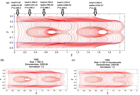
In Fig.6, different instants of the filling process predicted by the Stokes–Darcy (S–D) and Stokes–Brinkman (S–B) approaches are compared; in each instant, the fluid front posi-tion along the channel is the same for both approaches, S–D and S–B, but different evolution times are predicted. The fluid front shapes at the first instant look very similar for both approaches (Fig.6a vs. b), with S–D predicting a slightly
greater arrival time than S–B. As expected, due to the low value of the capillary ratio considered,Ccap =1×10⁻², the
fluid fronts in the channel surpass the fluid front in the tow, and, after a while, the liquid completely surrounds the first weft, see Fig.6e, f. At the instant corresponding to Fig.6c, d, when the liquid at the channel is approximately half the way along the first weft, 6.57% of the total filling time has elapsed according to S–D, while S–B predicts a value of 5.78%. Additionally, the minimum position of the fluid front in both the warps and the weft is barely larger for the S–D simulation. When the channel fluid fronts totally surround the first weft and merge one another, the air is trapped and the void compression starts. According to Fig.6e, f, the fluid fronts in the warps and the weft for S–D are ahead with respect to S–B, resulting in a smaller initial void (bubble) in the case of S–D. Moreover, the real arrival time to this position is longer for S–B, but the normalized time is shorter instead. This last feature is common for all the cases ana-lyzed in Fig.6a–h, where the normalized times of the fluid front evolution are always shorter for the S–B simulation. Figure6g, h corresponds to the case when the fluid front in the channel is approximately at 80% of the total length of the domain; at this point of the simulation, the time in the S–D approach is 57.2% of the total evolution time, while the time in S–B is 54.7%. This is a manifestation of the reduction of the saturation rate as the fluid front progresses with respect to the initial rate, as it is confirmed later. When the channel fluid front totally surrounds the second weft another bubble is formed, undergoing a compression process until the partial equilibrium is attained (see Fig.6i, j), as in the first bubble. In these last two figures, it can be observed that the voids predicted by the S–D simulation are smaller than those ones predicted by S–B, with the bubble of the first weft smaller than the one of the second weft for both approaches. In gen-eral, the influence of the type of approach, S–D or S–B, on the void location is not as significant as the influence on the void size and shape, for more details see Table4
4.3.3 Effect of the capillary ratio on the void characterization
Let us now consider the effect of the capillary ratio on the characterization of the voids (size, shape and location) formed in the first and second weft, and the differences among these voids when they are predicted by the two formulations considered here, S–D and S–B. In our analysis three different capillary ratios are considered:Ccap =1×10⁻², Ccap =
1×10⁻¹andCcap =5×10⁻¹; the solutions and
correspond-ing analysis for the former capillary ratio,Ccap=1×10⁻²,
Table 4 Characterization of final voids for S–B withβ=1.24 and S–D withγ=1.27
Approach Capillary ratio Void of first weft Void of second weft
Size* Shape Location Size* Shape Location
Stokes–Brinkman 1.00×10⁻² 7.58×10⁻³ 2.34 9.48×10⁻¹ 9.87×10⁻³ 1.93 9.35×10⁻¹ 1.00×10⁻¹ 1.08×10⁻² 2.84 9.83×10⁻¹ 6.55×10⁻³ 3.32 9.87×10⁻¹
5.00×10⁻¹ 1.97×10⁻³ 4.24 9.65×10⁻¹ 0.00 NA NA
Stokes–Darcy 1.00×10⁻² 5.08×10⁻³ 2.10 9.32×10⁻¹ 8.01×10⁻³ 1.86 9.46×10⁻¹ 1.00×10⁻¹ 1.07×10⁻² 3.10 9.84×10⁻¹ 7.34×10⁻³ 3.59 9.91×10⁻¹ 5.00×10⁻¹ 4.94×10⁻³ 4.17 9.78×10⁻¹ 2.45×10⁻³ 5.21 9.66×10⁻¹
Pcap,max =2σcos(θ) (1−εt) / (Rεt) (76)
Consequently, in all the cases considered here, where the values ofσ, θ, Rand εt are kept constants, the value of the
maximum capillary pressure, Pcap,max, is always the same
and therefore different values of the capillary ratio,Ccap,
corresponds to different values of the inlet pressure given by:Pi n=Pcap,max/Ccap.
As it was observed before in Fig.6i (S–B) and j (S–D), forCcap =1×10⁻²the bubble of the first weft is smaller
than the one of the second weft. In such case, this happens because the first bubble supports a higher pressure consider-ing that it is closer to the inlet and consequently experiences a higher compression. The values of the compressibility ratios obtained with both formulations, S–D and S–B, are: for the bubble of the first weft,ψ =0.512 (S–B) andψ = 0.587 (S–D), whereas, for the second one,ψ =0.304 (S–B) and
ψ=0.332 (S–D). Figure7a–d show the results for the other two values of the capillary ratio (Ccap = 1×10⁻¹ and Ccap =5×10⁻¹), where the flow in the channel has advanced
enough to allow the formation of the bubbles in both wefts. For these two cases ofCcap, the bubble at the first weft is
larger than the one at the second weft for both formulations, S–B and S–D, which is opposite to the case described before forCcap =1×10⁻², where the second bubble was larger
than the first one. This apparent unexpected behavior is due to the larger values of the capillary ratio considered in these last two cases,Ccap =1×10⁻¹ andCcap =5×10⁻¹, in
comparison withCcap =1×10⁻². From the previous
anal-ysis of the maximum capillary pressure it follows that when
Pcap,maxis constant, as in the present cases, larger values of
the capillary ratio,Ccap, correspond to lower values of the
inlet pressure,Pi n. At lower inlet pressure, the fluid fronts at
the channel move more slowly; besides, the capillary forces always promote the weft impregnation. These two simultane-ous effects result in smaller differences between the location of the fluid fronts at the channel and the location of the fluid front at the wefts before the channel fluid fronts enclose the wefts, and, consequently, in smaller initial bubbles, asCcap
is higher. This consequence is in turn more pronounced at
the second weft due to the slower channel flow velocities obtained there regarding the ones obtained in the first weft, given the increase of the flow resistance as the fluid front pro-gresses; accordingly, the initial void size at the second weft will be smaller than the one at the first weft. On the other hand, at a lower inlet pressure, the bubbles are subjected to lower compression, and consequently, at larger values of the capillary ratio (Ccap = 1×10⁻¹andCcap = 5×10⁻¹),
the initial void size is very similar to the final void size for both wefts; as the initial void is smaller for the second weft, the final void is too, as can be observed in Fig.7for both approaches, S–B and S–D.
The results of the void characterization obtained with both formulations, S–D and S–B, are summarized in Table 4, for all values ofCcap considered. As can be observed from
that table, the largest voids in the first weft are obtained for
Ccap=1×10⁻¹in both formulations and the smallest ones,
forCcap = 5×10⁻¹, with the void size corresponding to Ccap=1×10⁻²in between them. On the other hand, for the
second weft, the void is always smaller asCcapis higher, with
no void formation,Si ze∗ =0, forCcap =5×10⁻¹when
using the S–B approach (see Fig.7c), while S–D predicts the formation of a very small bubble (see Fig. 7d). Regarding the void shape, the increase ofCcap generates bubbles with
a higher aspect ratio for both wefts using both approaches, S–D and S–B.
4.3.4 Comparison of saturation curves
The time evolution of the saturation curves predicted by the S–D and S–B approaches for the three capillary ratios are compared in Fig.8a, where it can be observed a similar gen-eral behavior for all curves. Figure8b shows the saturation curve obtained with the S–D simulation forCcap=1×10⁻¹
Fig. 7 Total fillings of RUC’s.aCcap=1×10⁻¹(Stokes–Brinkman,
β=1.24),bCcap=1×10⁻¹(Stokes–Darcy,γ =1.27),c Ccap=
5×10⁻¹(Stokes–Brinkman,β=1.24),d Ccap=5×10⁻¹(Stokes–
Darcy,γ =1.27)
point (1), the saturation rate decreases until the merging of the channel fluid fronts (from 1 to 2) due to the flow resistance exerted by the first weft. When the channel fluid fronts have surrounded the first weft and encountered one another, point (2), an increase of the saturation rate can be noticed. This rate is kept almost constant until the arrival of the fluid front to the second weft (from 2 to 3), moment from which the sat-uration rate progressively decreases again until the second
Fig. 8 Saturation curves.aComparisson Stokes–Brinkman withβ=
1.24 versus Stokes–Darcy withγ =1.27.bStokes–Darcy forCcap=
1×10⁻¹
merging of the fluid fronts (from 3 to 4) due to the resis-tance exerted by the second weft. In point (4), saturation rate barely increases, and from (4) to the end of simulation (5), saturation rate is essentially constant. The nearly constant saturation rate between 2 and 3 is expected since no porous obstacles are present in the channel between these points, in contrast with what happens between the points 1 to 2 and 3 to 4, where the saturation rate decreases due to the presence of the first and second weft, respectively.
According to Fig.8a, forCcap =1×10⁻²andCcap =
1×10⁻¹, the saturation curves predicted by both approaches (S–D and S–B) are almost identical, but the final saturation is slightly higher for the S–D result (see detail in Fig. 8a). The highest differences between the saturation curves of both approaches (S–D and S–B) are observed forCcap=5×10⁻¹,
where the capillary effects are the most relevant; in this case, the final RUC saturation is barely higher for the S–B scheme (see detail in Fig.8a).
4.4 Influence of matching conditions on the void formation for the Stokes–Brinkman approach
4.4.1 Influence of the jump stress coefficient
[image:17.595.310.541.51.313.2] [image:17.595.56.288.52.544.2]Fig. 9 Total fillings of RUC’s for Stokes–Brinkman withβ=0.7.aCcap=1×10⁻²,b Ccap=1×10⁻¹,cCcap=5×10⁻¹
Table 5 Influence ofβandCcapon the void size
Capillary ratio Void size
First weft Second weft Total
β=1.24 β=0.70 β=1.24 β=0.70 β=1.24 β=0.70
1.00×10⁻² 7.582×10⁻³ 6.573×10⁻³ 9.866×10⁻³ 8.796×10⁻³ 1.745×10⁻² 1.537×10⁻² 1.00×10⁻¹ 1.077×10⁻² 1.039×10⁻² 6.548×10⁻³ 2.150×10⁻³ 1.732×10⁻² 1.254×10⁻² 5.00×10⁻¹ 1.973×10⁻³ 1.927×10⁻³ 0.00 0.00 1.973×10⁻³ 1.927×10⁻³
three different values of Ccapconsidered here. The total
fill-ings of the RUC for Serie 1 and the different values of Ccap
were already analyzed in the previous section and reported in Fig.6i (Ccap=1×10⁻²), 7a (Ccap =1×10⁻¹), and
7c (Ccap = 5×10⁻¹). Equivalent results for Serie 2 are
shown in Fig.9a–c, where, in the case ofCcap =1×10⁻²
(Fig.9a), different fluid fronts with positions in the channel corresponding to the same ones reported in the first column of Fig.6for the Serie 1 are highlighted using arrows. As can be seen from these figures (first column of Figs.6and9a), the real, dimensionless and normalized arrival times correspond-ing to these positions are shorter forβ =0.70 (Fig.9a).
In Table5, the effect of Ccapon the void size at the first and
second wefts for both values ofβ(β =1.24 andβ =0.70)
is presented, with the smaller voids found forβ =0.70 in both wefts; the void size difference between both values of
β is less significant for Ccap = 5 ×10⁻¹, i.e. the larger
capillary ratio examined here. Although the size of the first bubble is not a monotonic function ofCcapfor both values of β, with the smaller voids corresponding toCcap =5×10⁻¹
and the larger ones, to Ccap = 1 ×10⁻¹, the size of the
second bubble is a decreasing monotonic function ofCcap,
and the resulting total void size, which is the sum of the size of both bubbles, also decreases withCcap. This last behavior
[image:18.595.53.543.434.522.2]