Katarzyna Macieszczak,1, 2 M˘ad˘alin Gut¸˘a,1 Igor Lesanovsky,2 and Juan P. Garrahan2
1School of Mathematical Sciences, University of Nottingham, Nottingham, NG7 2RD, UK 2
School of Physics and Astronomy, University of Nottingham, Nottingham, NG7 2RD, UK
(Dated: June 23, 2016)
By generalising concepts from classical stochastic dynamics, we establish the basis for a the-ory of metastability in Markovian open quantum systems. Partial relaxation into long-lived metastable states—distinct from the asymptotic stationary state—is a manifestation of a separation of timescales due to a splitting in the spectrum of the generator of the dynamics. We show here how to exploit this spectral structure to obtain a low dimensional approximation to the dynamics in terms of motion in a manifold of metastable states constructed from the low-lying eigenmatrices of the generator. We argue that the metastable manifold is in general composed of disjoint states, noiseless subsystems and decoherence-free subspaces.
Introduction. Stochastic many-body systems often dis-play complex and slow relaxation towards a stationary state. A common phenomenon is that of metastabil-ity, where initial relaxation is into long-lived states, with subsequent decay to true stationarity occurring at much longer times. This separation of times in the dynamics has evident experimental manifestations, for example in two-step decay of time correlation functions. Metastabil-ity is a common occurrence in classical soft matter [1], glasses being the paradigmatic example [2, 3].
There is much current interest in the non-equilibrium dynamics of quantum many-body systems, both closed (i.e., isolated) and open (i.e., interacting with an envi-ronment). This includes issues such as thermalisation [4– 7], many-body localisation [8–10], and aging and glassy behaviour, where questions about timescales and partial versus full relaxation play central roles [11–16]. From the quantum information perspective, decoherence free sub-spaces [17–20] and noiseless subsystems [21–23], where parts of the Hilbert space are protected against exter-nal noise, are ideal scenarios for implementing quantum information processing [24]. Since experiments are per-formed in finite time, it is sufficient (and practical) to consider manifolds of coherent states which are only sta-ble over experimental timescales, i.e., metastasta-ble, with respect to noise.
Given this broad range of problems, it would be highly desirable to have a unified theory of quantum metastabil-ity. In this paper we lay the ground for such a theory for the case of open quantum systems evolving with Marko-vian dynamics. Our starting point is a well-established approach for metastability in classical stochastic systems [25–29]. We develop an analogous method for quantum Markovian systems based on the spectral properties of the generator of the dynamics. Separation of timescales implies a splitting in the spectrum, and this spectral di-vision allows us to construct metastable states from the low-lying eigenmatrices of the generator. Based on per-turbative calculations for finite systems, we argue that the manifold of metastable states is in general composed of disjoint states, noiseless subsystems and
decoherence-free subspaces. We illustrate these possibilities with sim-ple examsim-ples. We further discuss how to reduce the overall dynamics to a low-dimensional effective motion in the metastable manifold, and consider the associated behaviour of time correlations.
Quantum metastability and spectral properties. We consider an open quantum system evolving under Markovian dynamics, with Linbladian master equation
d
dtρ(t) = Lρ(t) [30–33], where the generator of the dy-namicsL is,
L(·) :=−i[H,(·)] +X j
Jj(·)Jj†− 1 2{J
† jJj,(·)}
. (1)
The state of the system at time t is ρ(t), the sys-tem Hamiltonian is H, and {Jj} are quantum jump operators [34]. While in general the linear operator L is not diagonalisable, one can find its eigenvalues {λk, k= 1,2, . . .}[which we order by decreasing real part, Re(λk)≥Re(λk+1)] each corresponding to an eigenspace
or a Jordan block. SinceLgenerates a proper quantum stochastic (completely positive trace-preserving) dynam-ics ofρ(t), its largest eigenvalue vanishes,λ1= 0, and its
associated right eigenmatrix R1 is the stationary state,
R1 =ρss (the corresponding left eigenmatrix being the
identity, L1 = I) [35]. The real parts of eigenvalues
{λk>1} give the relaxation rates of all the modes of the
system dynamics. In particular, the second eigenvalue λ2 determines the spectral gap, whose inverse is related
to the longest timescaleτ of the relaxation of the system to the stationary state, i.e., kρ(t)−ρssk ∼ e−t/τ with
τ∼1/|Re(λ2)| (wherekAk:= Tr
√ A†A).
Metastability manifests as a long time regime when the system appears stationary, before eventually relaxing to ρss. This occurs when low lying eigenvalues become
separated from the rest of the spectrum. Lets assume that this separation occurs between them-th mode and the rest, that is, |Re(λm)| |Re(λm+1)|. We can then
⌦
1⌦
2|
0
i
|
1
i
|
2
i
(a)
(b)
0
Re( )⌦1 2⌦1 3⌦1
˜
⇢
1˜
⇢
2⇢
ss(c)
⌦1t
1 10Á 102 103Ê 104 105 W1t
(d)
(e)
C ( t )1 10 102 103 104 105 W1t
0.2 0.4 0.6 0.8 1.0 · ‡
ÛÁ Ê Ú
W2êW1=1ê100
W2êW1=1ê50
W2êW1=1ê25
⌦1t
1 10 102 103 104 105 W1t
0.2 0.4 0.6 0.8 1.0 · ‡
ÛÁ Ê Ú
[image:2.612.82.272.57.274.2]W2êW1=1ê100 W2êW1=1ê50 W2êW1=1ê25
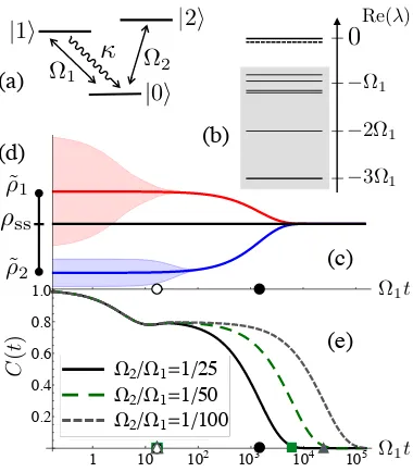
FIG. 1. Example of metastability in a 3-level system:
(a) Level scheme and transitions. (b) Spectrum ofLshowing separation of timescales between (λ1, λ2) (full and dashed)
and {λk>2} (shaded), for the case κ = 4Ω1, Ω2 = Ω1/10.
(c) Illustration of the distance of the state,ρ(t), to the MM. We considerρ(t) starting from pure states corresponding to the eigenvectors ofL2 with maximal (top/red) and minimal
eigenvalues (bottom/blue)cmax2 andcmin2 . The full curves
in-dicate the nearest state on the MM,ρMS(t), to the full state
ρ(t). The shaded region indicates the scale of the “error”
kδρ(t)k with δρ(t) := ρ(t)−ρMS(t). On times of order τ00
(open circle) the state ρ(t) relaxes to the MM (in this case to either of the eMS,eρ1,2), as seen by the shaded region
de-creasing to zero. On times of orderτ (filled circle) there is an eventual relaxation to the stationary stateρss (central/black
line). Sincem= 2, in this caseτ0=τ. (d) The MM is a one-dimensional simplex. (e) Normalised autocorrelation, C(t), of the observable|1ih1| − |2ih2|, in the stationary state. For decreasing Ω2/Ω1 (i.e., decreasing gap), metastability in the
regimeτ00(open symbols) toτ (filled symbols) is increasingly pronounced.
write for the time evolution from an initial stateρin,
ρ(t) =etLρin=ρss+
m X
k=2
etλkc
kRk+
etL
I−Pρin, (2)
where ck = Tr(Lkρin) are coefficients of the initial state
decomposition into the eigenbasis of L [35]. In (2) we have introduced the projectionP on the subspace of the firstmeigenmatrices,Pρ:=ρssTr(ρ)+Pmk=2RkTr(Lkρ), and
etL
P := Pe tL
P. Expanding the exponentials in the sum, and assumingλ1, . . . , λm are real, Eq. (2) can be rewritten as [36],
ρ(t) =ρss+
m X
k=2
ckRk
+O(k[tL]Pk) +O etL I−P . (3)
Dynamics will appear stationary foranyinitial condition when the last two terms are small. This defines a range τ00tτ0 where metastability occurs. Intuitively the last term can be discarded ifτ00∼1/|Re(λ
m+1)|and the
overlap of the initial state with the suppressed modes is not too large, so that the sum over many modes of small amplitude can be neglected. Thus, for times τ00
t
the system relaxes into a state in the metastable mani-fold(MM). Apparent stationarity requiresk[tL]Pk 1, which defines the upper limit of the metastable interval: τ0
∼1/|Re(λm)|(formnot too large).
More generally, eigenvalues could be complex, appear-ing in conjugate pairs,λk,1=λ∗k,2, with imaginary parts
that cannot be discarded. Taking this into account, a stateρMS in the MM would read in general [37],
ρMS=ρss+
m X
k
c0k(t)R0k. (4)
Whenλk is real, we have thatc0k(t) :=ck andR0k:=Rk. For conjugate pairs,λk,1=λ∗k,2, we have thatck,1=c∗k,2
andc0
k,1:=|ck,1|cos(ωkt+δk) andc0k,2:=|ck,2|sin(ωkt+ δk), whereR0k,1:=Rk,1+Rk,2andR0k,2:=i(Rk,1−Rk,2),
withδk := arg(ck),ωk:= Im(λk). In Eq. (4) we have dis-carded the second line of Eq. (14), which leadsρMSto be
approximately positive with its negative part bounded by the corrections to the invariance of the MM in Eq. (14). The remaining time dependence in Eq. (4) constitutes rotations within the MM that leave the MM invariant, which necessarily correspond to non-dissipative evolution forτ00
tτ0, which we also discuss below.
Beyond the metastable regime, t &τ0, dynamics will correspond to motion in the MM towards the true sta-tionary state, which is reached at times t τ. This effective dimensional reduction due to a separation of timescales is a key result of this paper.
Geometrical description of quantum metastabil-ity. The MM can be described geometrically by gen-eralising the classical method of Refs. [25–29]. In the metastable regime the system state is well approximated by a linear combination of the m low-lying modes, see Eqs. (4). A metastable state is determined by a vec-tor (c0
2, . . . , c0m) in Rm−1. We thus refer to the MM as being (m−1)-dimensional, but note that each point on this manifold represents aD2density matrixρ
MS, where
D= dim(H) is the dimension of the Hilbert space Hof the system. Furthermore, the MM is a convex set as it is a linearly transformed convex set of initial statesρin.
Let us first consider the case of m = 2. Due to the convexity of the MM, any metastable state is a mixture ofextreme metastable states(eMS). In this case they are just two,ρe1 andρe2, obtained from
e
ρ1=ρss+cmax2 R2, ρe2=ρss+c
min
2 R2, (5)
where cmax
2 , cmin2 are the maximal and minimal
positive despiteR2 being non-positive. From Eq. (14) it
follows, up to corrections, thatρ(t) =p1ρe1+p2ρe2 with probabilitiesp1,2= Tr(Pe1,2ρin) where
e
P1= L2−cmin2 I
/∆c2, Pe2= (−L2+cmax2 I)/∆c2,
and ∆c2 :=cmax2 −cmin2 . Note that the observables Pe1,2
satisfyPe1,2 ≥0 and Pe1+Pe2 =I. This leads to eρ1 and
e
ρ2being (approximately) disjoint [38].
Example I: 3-level system. Consider the 3-level system of Fig. 1(a), with HamiltonianH= Ω1(|1ih0|+|0ih1|) +
Ω2(|2ih0|+|0ih2|) and jump operator J = √κ|0ih1|.
When Ω2 Ω1, dynamics can be “shelved” for long
times in |2i, giving rise to intermittency in quantum jumps [32], which can be seen as coexistence of “active” and “inactive” dynamical phases [39]. Figure 1(b) shows the spectrum ofL: the gap is small for Ω2Ω1, the two
leading eigenvalues detach from the rest (i.e., m = 2), and the dynamics is metastable. Figure 1(c) illustrates the trace distance of the state ρ(t) to the MM start-ing from ρin 6= ρss: an initial decay on times of order
of τ00 to the nearest point on the MM (in this case to an eMS) is followed by decay to ρss on times of order
τ0 = τ (since m = 2). The MM for this m = 2 case is a one-dimensional simplex (i.e., a convex set whose in-terior points uniquely represent probability distributions on the vertices), see Fig. 1(d).
Form >2 the convex set MM of possible coefficients can have more thanmextreme points. For classical dy-namics it has been proven that this set is well approxi-mated by a simplex [27], whose vertices correspond tom disjoint eMS and its barycentric coordinates to the prob-abilities of a metastable state decomposed as a mixture of the eMS, cf. Fig. 1(d). For quantum dynamics and m >3, we expect the structure of the MM to be richer than just a simplex. As we describe below, the MM can in general also include decoherent free subspaces (DFS) [17–19] and noiseless subsystems (NSS) [21, 22] which are protected from dissipation in the metastable regime, as the next example shows.
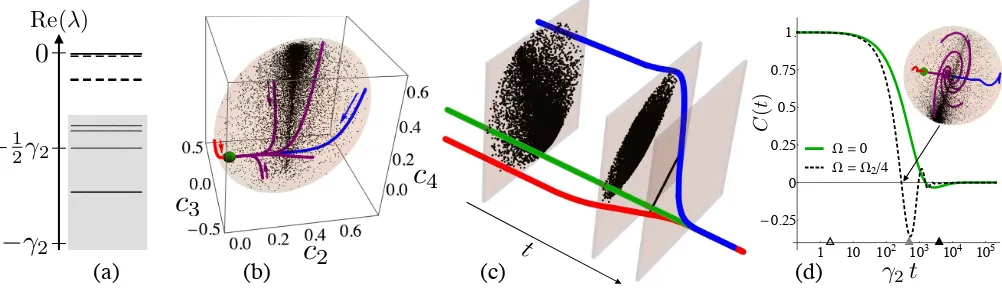
Example II: Collective dissipation and a metastable DFS.
Consider a two-qubit system with Hamiltonian H = Ω1σ1x + Ω2σ2x, and a collective jump operator J =
√γ
1n1σ2−+√γ2(1−n1)σ+2. When Ω1,2 γ1,2 there
is a small gap and the four leading eigenvalues of L de-tach from the rest, Fig. 2(a). This is related to the fact that any superposition of|01iand|10iis annihilated by J. Fig. 2(b) maps out the MM by randomly sampling all (pure) initial states ρin from Hand obtaining their
cor-responding metastable state via Eq. (4): the MM is an affinely transformed Bloch ball corresponding to a DFS qubit within the metastable regime τ00
t τ0. It important to note: (i) this coherent structure is not the consequence of a symmetry, as for γ1 6= γ2 the system
dynamics neither has a U(2) nor an up-down nor a
per-mutation symmetry, cf. [40]; (ii) the smallestmfor which we can obtain a DFS ism= 4, as in this case.
Structure of metastable manifold. We aim to find the general structure of the MM for two classes of systems for whichLhas a small gap: (A) finite systems where the gap closes at some limiting values of the parameters inL (such as Ω2→0 in Example I, and Ω1,2→0 in Example
II); (B) scalable systems of sizeN where the gap closes only in the thermodynamic limitN → ∞ (such as the dissipative Ising model of Ref. [43]).
For class A we prove via non-Hermitian degenerate per-turbation theory [38] that the structure of a metastable stateρMS ∈MM is given by the following block structure,
ρMS =
m0 X
l=1
plρel⊗ωl+ corrections, (6)
withHbeing the orthogonal sumH=L
lHl⊗Kl, where e
ρlare fixed states onHl(cf. eMS above),ωlare arbitrary states onKl, andpl are probabilities. Up to the correc-tions, this is a general structure of a manifold of station-ary states of open quantum Markovian dynamics [44]. The metastable regime is given by τ0 t s−2τ0,
whereτ0 is the relaxation time for the unperturbed
dy-namics ands is the scale of the perturbation [38]. The corrections in Eq. (6) are of the order of the corrections to the invariance of the MM during the metastable time regime, cf. Eq. (14). The (m−1) coefficients (c0
2, . . . , c0m) that determine ρMS, see Eq. (4), correspond
approxi-mately to an affine transformation of the m entries of plωl (l = 1, . . . , m0) in Eq. (6) with
Pm0
l=1pl = 1 [38]. Therefore, the MM approximately represents the degrees of freedom of the classical-quantum space in Eq. (6).
For class B we conjecture that the coefficients rep-resenting the MM converge to degrees of freedom of a classical-quantum space as in Eq. (6), when the separa-tion in the spectrum becomes more and more pronounced as N → ∞. Note that the dimensionality of the MM does not change withN and thus the convergence is well defined. This general conjecture is based on the neces-sary conditionthat the low-lying spectrum ofLfeatures only trivial Jordan blocks [45]. Note that a conjecture of theρMSstructure being approximately that of stationary
states, cf. Eq. (6), is a stronger claim. A proof of the former conjecture for class B appears challenging at this moment, see comment in [38].
0
t
(a)
(b)
(c)
(d)
1 10 102 103 104 105 g2t
1.
0.75
0.5
0.25
0
-0.25
Û Ú Ú
W = W2ê4
W =0
2
t
C
(
t
)
Re( )
0
1 2 2
2
.
5
.
5
0
0
.
4
.
4
.
6
.
2
.
2
.
6
c
2
[image:4.612.59.560.56.203.2]c
4
c
3
FIG. 2. Example of a coherent metastable manifold:(a) Spectrum ofLfor Example II (atγ1= 4γ2, Ω1= 2Ω2=γ2/50).
The first four eigenvalues (m= 4) split from the rest (shaded) and define the MM. Note the further splitting between (λ1, λ2)
and (λ3, λ4) (which are almost degenerate). (b) The MM is a qubit. Dots represent the metastable states reached from random
initial pure states. They map out under Eq. (4) an affinely transformed Bloch ball (shaded). The large dot (green) is ρss;
curves indicate paths in the MM taken by the states evolving from the extreme eigenvectors of L2 (red and blue), L3 and
L4 (purple) towardsρss. (c) Time evolution in the MM (affinely transformed to a Bloch ball—planes are projections in the
direction of the eigenbasis of ρss and another orthogonal direction): the MM contracts towards a one-dimensional simplex
before relaxing eventually toρss, due to the splitting of between the first two eigenvalues and the next two, see panel (a). (d)
Normalised auto-correlationC(t) for the observableσz1−σ z
2 (green/solid). Same for the case where there is an extra perturbing
Hamiltonian ∆H= Ωσ1x⊗σ2xwhich induces a rotation in the MM, manifesting in oscillations inC(t) in the metastable regime
(black/dashed). This realises in a metastable system the proposal of [41, 42] for implementing operations in a DFS.
and dim(Hl) > 1, Kl is also protected from noise and termed a noisless subsystem (NSS). The structures (ii) and (iii) correspond to quantum degrees of freedom (ωl) and do not appear in the case of classical dynamics [27]. In general the number of blocks in Eq. (6) is m0
≤ m, with equality occurring only when there are no DFS or NSS.
Effective motion in the metastable manifold. In the metastable regime, τ00
t τ0, metastable states appear stationary, or perhaps rotate within the MM. This latter case corresponds to either: (i) coherent motion in the DFS/NSS where the matricesωlof Eq. (6) evolve uni-tarily in time; or (ii) classical rotations with a frequency which is limited by the dimensionality of MM [46]. For class A systems only case (i) is possible [38, 41, 42].
For longer times, t &τ0, the MM contracts exponen-tially towards ρss. This is illustrated in Fig. 2(c) for
Example II. This low dimensional evolution in the MM is well described by an effective generatorLeff := [L]P,
which can be considered as the generator of the dynamics averaged over intervalsτ00. If the MM is approximately a simplex (i.e., containing no DFS or NSS) the motion generated byLeff is that of classical transitions between macrostates described by the eMS (see [38] for m = 2 and [47] for the general case). For class A when the MM contains coherent subsystems/subspaces, the mo-tion preserves the structure of Eq. (6) and can be shown to be trace-preserving and approximately completely-positive [38, 48, 49]. Note that decoupling of (slower) classical dynamics from (faster) quantum evolution in the
MM requires further separation in low-lying eigenvalues ofL. This is illustrated in Fig. 2(c) for Example II.
In practice, metastability can be accessed through the connected auto-correlation [14] of the measurement M of a system observable, even in the stationary state, C(t) := Tr(MetLMρss)−Tr(Mρss)2[50]; see Figs. 1(e),
2(d). The first measurement M perturbs ρss, and the
state conditioned on the result partially relaxes towards the MM fort.τ00. In the metastable regime correlations will persist as the different blocks in (6) do not communi-cate, and for the case where all low-lying eigenvalues are real,C(t)≈Tr(MPMρss)−Tr(Mρss)2. When low-lying
eigenvalues are complex, oscillations ofC(t) can occur in the metastable regime, as in Fig. 2(d). When t & τ0, dynamics begins to relax back towards ρss, erasing all
information about the initial result,C(t)≈0, fortτ. Outlook. The next steps in the development of the the-ory of quantum metastability presented here include:
(i) For many-body systems, where direct diagonalisa-tion ofLis impractical, it should be possible to use dy-namical large-deviation methods [51] to identify dynam-ically the different blocks in Eq. (6) by biasing ensembles of quantum trajectories [39]. This approach could be implemented numerically by generalising classical path sampling [52] and/or cloning techniques [53].
interesting to consider more broadly DFS that do no arise as a consequence of symmetry, cf. Example II above.
(iii) We have considered here metastability in the case of Markovian dynamics generated by a Lindbla-dianL. Metastability occurs also when dynamics is non-Markovian, see e.g. [54]. It should be possible to gener-alise the method introduced above to the non-Markovian case of a time-dependent generatorL(t).
(iv) A significant challenge is to extend the ideas pre-sented here to study metastability inclosedquantum sys-tems. This would be relevant to the fundamental prob-lems of thermalisation [5] and many-body localisation [8]. This work was supported by EPSRC Grant No. EP/J009776/1 and ERC Grant Agreement No. 335266 (ESCQUMA). K.M. thanks M. Idel for discussions.
[1] K. Binder and W. Kob,Glassy Materials and Disordered Solids (World Scientific, 2011).
[2] G. Biroli and J. P. Garrahan, J. Chem. Phys. 138, 12A301 (2013).
[3] L. Berthier and M. D. Ediger, Physics Today 69, 40 (2016).
[4] A. Polkovnikov, K. Sengupta, A. Silva, and M. Ven-galattore, Rev. Mod. Phys.83, 863 (2011).
[5] J. Eisert, M. Friesdorf, and C. Gogolin, Nature Physics
11, 7 (2014).
[6] L. D’Alessio, Y. Kafri, A. Polkovnikov, and M. Rigol, arXiv:1509.06411.
[7] C. Gogolin and J. Eisert, Reports on Progress in Physics
79, 056001 (2016).
[8] R. Nandkishore and D. A. Huse, Annu. Rev. Condens. Matter Phys.6, 15 (2015).
[9] N. Y. Yao, C. R. Laumann, J. I. Cirac, M. D. Lukin, and J. E. Moore, arXiv:1410.7407.
[10] W. De Roeck and F. Huveneers, Phys. Rev. B90, 165137 (2014).
[11] T. Prosen, Phys. Rev. Lett.106, 217206 (2011). [12] T. E. Markland, J. A. Morrone, B. J. Berne, K. Miyazaki,
E. Rabani, and D. R. Reichman, Nature Phys.7, 134 (2011).
[13] B. Olmos, I. Lesanovsky, and J. P. Garrahan, Phys. Rev. Lett.109, 020403 (2012).
[14] B. Sciolla, D. Poletti, and C. Kollath, Phys. Rev. Lett.
114, 170401 (2015).
[15] M. van Horssen, E. Levi, and J. P. Garrahan, Phys. Rev. B92, 100305 (2015).
[16] M. Znidaric, Phys. Rev. E92, 042143 (2015).
[17] P. Zanardi and M. Rasetti, Phys. Rev. Lett. 79, 3306 (1997).
[18] P. Zanardi, Phys. Rev. A56, 4445 (1997).
[19] D. A. Lidar, I. L. Chuang, and K. B. Whaley, Phys. Rev. Lett.81, 2594 (1998).
[20] D. Kielpinski, V. Meyer, M. Rowe, C. Sackett, W. Itano, C. Monroe, and D. Wineland, Science291, 1013 (2001). [21] E. Knill, R. Laflamme, and L. Viola, Phys. Rev. Lett.
84, 2525 (2000).
[22] P. Zanardi, Phys. Rev. A63, 012301 (2000).
[23] L. Viola, E. M. Fortunato, M. A. Pravia, E. Knill,
R. Laflamme, and D. G. Cory, Science293, 2059 (2001). [24] M. A. Nielsen and I. Chuang, Quantum Information.
Cambridge University Press, Cambridge (2000). [25] B. Gaveau and L. S. Schulman, J. Mat. Phys.37, 3897
(1996); 39, 1517 (1998); J. Phys. A20, 2865 (1999). [26] A. Bovier, M. Eckhoff, V. Gayrard, and M. Klein,
Comm. Math. Phys228, 219 (2002).
[27] B. Gaveau and L. S. Schulman, Phys. Rev. E73(2006). [28] S. Nicholson, L. Schulman, and E. Kim, Phys. Lett. A
377, 1810 (2013).
[29] For a pedagogical review see: J. Kurchan,
arXiv:0901.1271.
[30] G. Lindblad, Comm. Math. Phys48, 119 (1976). [31] V. Gorini, A. Kossakowski, and E. C. G. Sudarshan, J.
Mat. Phys.17, 821 (1976).
[32] M. B. Plenio and P. L. Knight, Rev. Mod. Phys.70, 101 (1998).
[33] C. Gardiner and P. Zoller, Quantum noise (Springer, 2004).
[34] Calligraphic font denotes super-operators, such as the generatorL, while Roman font denotes normal operators, such as the HamiltonianH or the jump operatorsJi.
[35]RkandLkare right and left eigenmatrices ofLfor
eigen-value λk, i.e., L(Rk) = λkRk and L†(Lk) = λkLk. In
principle Rk 6= L †
k since in general L 6= L †
. Left and right eigenmatrices form a complete basis, which we nor-malise as Tr(LkRk0) = δk,k0. We assume there are no Jordan blocks in the part of the spectrum relevant for our analysis; see e.g. Ref. [27].
[36] The normk·kof a super-operatorS, is the norm induced by the trace norm,kAk:= Tr√A†A, of complex matrices Aon whichS acts: kSk:= supkAk=1TrkSAk.
[37] For real eigenvalues,Rk and Lk can be chosen
Hermi-tian. Note that while R1 =ρss, Rk>1 are not positive.
Complex eigenvalues come in conjugate pairsλk,1=λ∗k,2
and if so we haveRk,1=R†k,2,Lk,1=L†k,2.
[38] See Supplemental Material for derivations of (i) case m = 2: approximate disjointness of two EMSs and the effective classical dynamics. (ii) class A systems: the structure of the metastable manifold from Eq. (6), the metastable regime and the effective dynamics. (iii) class B systems: a comment on the conjecture.
[39] J. P. Garrahan and I. Lesanovsky, Phys. Rev. Lett.104, 160601 (2010).
[40] V. V. Albert and L. Jiang, Phys. Rev. A 89, 022118 (2014).
[41] P. Zanardi and L. Campos Venuti, Phys. Rev. Lett.113, 240406 (2014).
[42] P. Zanardi and L. Campos Venuti, Phys. Rev. A 91, 052324 (2015).
[43] C. Ates, B. Olmos, J. P. Garrahan, and I. Lesanovsky, Phys. Rev. A85, 043620 (2012).
[44] B. Baumgartner and H. Narnhofer, J. Phys. A41, 395303 (2008).
[45] Non-trivial Jordan blocks would lead to an unbounded norm ofρ(t) in the limit of gap→0 [56]. More precisely, Jordan blocks may be considered as long as they do not contribute significantly, so that Eq. (14) holds true with appropriately redefined corrections being small. This condition aims to exclude systems where a small gap is “accidental” in the sense it is unrelated to it vanishing in some limit.
as the low-lying eigenvalues ofLwere assumed all real. One can show [47] that the set of (c02, . . . , c
0
m) is again
a simplex. Points within the simplex evolve within it. Due to exponential shrinking, this evolution can allow for rotations, but with limited frequencies which decrease with decreasing gap.
[47] K. Macieszczak, M. Guta, I. Lesanovsky, and J. P. Gar-rahan, in preparation.
[48] P. Zanardi, J. Marshall, and L. Campos Venuti, Phys. Rev. A93, 022312 (2016).
[49] Z. Cai and T. Barthel, Phys. Rev. Lett. 111, 150403 (2013).
[50] For an observable M=PD
i=1mi|miihmi|, we have that
M(ρ) =PD
i=1mihmi|ρ|mii|miihmi|.
[51] H. Touchette, Phys. Rep.478, 1 (2009).
[52] L. O. Hedges, R. L. Jack, J. P. Garrahan, and D. Chan-dler, Science323, 1309 (2009).
[53] C. Giardina, J. Kurchan, V. Lecomte, and J. Tailleur, J. Stat. Phys.145, 787 (2011).
[54] M. Merkli, H. Song, and G. P. Berman, J. Phys. A48, 275304 (2015).
[55] A. Rosmanis, Linear Algebra and its Applications437, 1704 (2012).
[56] M. M. Wolf, Quantum channels and operations: Guided tour (2012)
SUPPLEMENTAL MATERIAL
Metastability for two low-lying eigenmodes
Here we consider the case ofm= 2 low-lying eigenvalues in the master operatorL, see Eqs. (1-4) in the main text.
Since the metastable manifold (MM) is convex and 1-dimensional, it is simply an interval and thus a simplex. Hence, any metastable state is a mixture of extreme metastable states (eMSs), in this case two: ρe1, ρe2. As a metastable state,ρMS=ρss+c2R2, is determined by the coefficientc2= Tr(L2ρin), the eMSs correspond to the extreme values
of c2 given by the maximum cmax2 and minimumcmin2 eigenvalue ofL2, see Eq. (5) in the main text. Furthermore,
note thatρe1,ρe2are the metastable states for the pure initial state given by theL2eigenvectors corresponding toc
max 2
and cmin
2 , respectively. As ρe1,ρe2 are then given by the truncated evolution equation (3) of the main text, we have Tr(ρe1,2) = 1 and eρ1,ρe2 are approximately positive with the corrections bounded by the corrections to stationarity in the metastable regime.
The decomposition ρMS = p1ρe1+p2ρe2 of a metastable state into the eMSs is given by the observables Pe1, Pe2 (for definition see the main text below Eq. (5)) which determine the probabilities asp1,2= Tr(Pe1,2ρin). We note that the
definition of ˜ρ1,2 and ρe1,2 insures that Tr(Peiρej) =δij for i, j = 1,2, andPe1,2 ≥0 and Pe1+Pe2 =1H, i.e., {Pek}
2
k=1
constitute a POVM.
Approximate disjointness of two eMS. Below we prove that the extreme metastable states are approximately disjoint. More precisely, we show that there is a division of the system Hilbert space H = H1 ⊕ H2 so that
Tr 1H1,2ρe1,2
≥1− O(C), whereC are the corrections to the stationarity in the metastable regime, cf. Eq. (3) in the main text.
Proof. Note that the stationary stateρss is a mixture of the two eMS,ρss =pss1 ρe1+p ss
2 ρe2, wherep ss
1 =−cmin2 /∆c2
andpss
2 =cmax2 /∆c2. We define the orthogonal subspacesH1 andH2 as follows,
H1= span{|ψki, k= 1, .., D: hψk|Pe1|ψki ≥pss1 }, (7)
H2= span{|ψki, k= 1, .., D: hψk|Pe2|ψki> pss2 }, (8)
where{|ψki}Dk=1is the orthonormal eigenbasis ofL2, which is also the eigenbasis of bothPe1andPe2. FromPe2=1−Pe1,
we have H =H1⊕ H2. Let |ψ1i and |ψ2i denote the eigenvectors of L2 corresponding to the extreme eigenvalues
cmax
2 and cmin2 . Let ρ1(t), ρ2(t) further be the system state at timet for the initial state chosen as|ψ1i,|ψ2i. From
the orthogonality of the eigenmatrices ofL(also in the case of Jordan blocks in I − P), it follows that
TrPe1ρ2(t)
= TrPe2ρ1(t)
=pss1 (e
tλ2−1). (9)
From positivity ofρ1(t) and the fact that 1H1 is diagonal in the eigenbasis ofPe1, we also have
TrPe1ρ2(t)
≥Tr1H1Pe1ρ2(t)
≥pss
Together with Eq. (9) it follows that
Tr (1H1ρe2)≤Tr (1H1ρ2(t)) +O(C)≤(e
tλ2−1) +O(C) =O(C), (11)
whereCare the corrections to the stationarity in the metastable regime, cf. Eq. (3). Analogously, Tr (1H2ρe1)≤ O(C), which ends the proof. Let us note that this argument is analogous to the case ofm= 2 in classical systems [1].
Effective classical dynamics in the metastable manifold. Here we consider the linear operator Leff := [L]P which governs the dynamics for timest&τ0. Note that in this case,m= 2, we have simplyτ =τ0= (
−Reλ2)−1.
Note that by the construction, the operatorLeff transforms the MM into itself. As for m= 2 the MM is a simplex,
Leff generates a positiveandprobability preserving evolution of the probabilities (p1(t), p2(t)). This implies thatLeff
is a generator ofclassical stochastic dynamics. Indeed, in the basis of extreme metastable states,ρe1,ρe2, we have
d dt
p1(t)
p2(t)
=Leff
p1(t)
p2(t)
= 1
∆c2
cmax
2 λ2 cmin2 λ2
−cmax
2 λ2 −cmin2 λ2
p1(t)
p2(t)
, (12)
where ∆c2 =cmax2 −cmin2 . We have thatλ2 <0 and cmin2 ≤0 due to Tr(L2ρss) = 0. Therefore it follows that Leff
indeed obeys the generator characteristics: the diagonal terms are negative, the off-diagonal terms are positive and the sum of entries in each column is 0. The corresponding dynamics is thus given by
p1(t)
p2(t)
=etLeff
p1
p2
= 1
∆c2
cmax
2 etλ2−cmin2 −cmin2 (1−etλ2)
cmax
2 (1−etλ2) cmax2 −cmin2 etλ2
p1
p2
, (13)
and for t → ∞ we obtain the probabilities corresponding to the stationary state, (−cmin 2 ρe1+c
max
2 ρe2)/∆c2 = ρss. The dynamics in (13) approximates the system dynamics with the corrections being bounded by the corrections to stationarity in the metastable regime (cf. Eq. (2) in the main text),
ρ(t) =etLρin=p1(t)ρe1+p2(t)ρe2+O
etL I−P
. (14)
Let us finally emphasize that for timest&τ0 dynamics takes place between eMSs, e
ρ1,ρe2, which can be considered as systemmacrostates in analogy to classical thermodynamics. The generator in Eq. (12) yields stochastic trajectories
of transitions between ρe1, ρe2. Those trajectories correspond to quantum trajectories coarse-grained in time over
intervals of the orderO(τ00), similarly as in the example of 3-level atom, see Fig. 1 in the main text, the intermittency in quantum jumps corresponds to conditional system dynamics being restricted to the dark level |2i (“inactive” dynamics) or the subspace spanned by the level|1iand|0i(“active” dynamics) [2].
Characterising the structure of the metastable manifold and effective dynamics for Class A systems
In this section we discuss metastablity of a finite open quantum system for which the gap closes at some value of parameters in the master equation (see Eq. (1) in the main text) so that the stationary state is no longer unique. For dynamics which are close to the degenerate case, we prove that there is a separation in the spectrum leading to a metastable time regime during which the system’s state has the structure given in Eq. (6) of the main text. Moreover, the effective dynamics in the metastable manifold is trace-preserving and approximately completely positive.
Perturbation theory analysis. We use the perturbation theory of linear operators (see Chapter 2 of [3]) in order to analyse an open quantum system of finite dimension whose Lindblad operator L(s) is obtained by perturbing a generatorL=L(0) featuring multiple stationary states. We considerLwithm-fold degeneracy of the stationary state manifold (SSM). In the proof we assume that the dynamics exhibits no rotations in the stationary state manifold, i.e. Lhas no non-zero imaginary eigenvalues. The case of unitarily rotating SSM can be analysed in a similar fashion [2]. Consequently, there are m right (left) eigenmatrices corresponding to the 0 eigenvalues, with no non-trivial Jordan blocks due to positive and trace-preserving dynamics [4]. The asymptotic states of L have the structure given by Eq. (6) in the main text (without the corrections), see e.g. [5]. We denote by P the projection on the SSM of L, with P(·) = Pml=10 ρl ⊗TrHl(1Hl⊗1Kl(·) ), so that for the initial state ρin, the asymptotic state is given by
pl= Tr(1Hl⊗1Klρin) andωl= TrHl(1Hl⊗1Klρin)/pl,l= 1, ..., m
For simplicity, we consider a linear perturbation of the Hamiltonian H(s) = H +sH(1), where H(1) is Hermitian,
and of the jumps operators are Jj(s) = Jj+sJ
(1)
j . The derivations below can be easily generalised to any analytic perturbation ofH andJj [3]. This leads to the following first- and second-order perturbation for the generator
L(s) =L+sL(1)+s2
L(2), where
L(1)=
−i[H(1),(·)] +X j
Jj(1)(·)J
† j −
1 2
n Jj†J
(1)
j ,(·) o
+ h.c.
L(2)=X j
Jj(1)(·)J
(1)
j †
−12
Jj(1) †
Jj(1),(·)
. (15)
We choose the dimensionless scale parametersso that that max(kL(1)
k,kL(2)
k) =O(τ−1), whereτ is the relaxation time forLdynamics (see below Eqs. (16)-(17) for the precise definition ofs).
From the perturbation theory of linear operators [3], the eigenvalues of the perturbed operatorL(s) are continuous with respect to s. Furthermore, if λ is an eigenvalue of L with algebraic multiplicity m, then for s small enough m eigenvalues of L(s) will cluster around the unperturbed eigenvalue λ. Those eigenvalues are referred to as the λ-group. In general the individual eigenvalues in theλ-group are not analytic in s, but correspond to branches of analytic functions. Moreover, the corresponding eigenmatrices may feature poles. However, the projection onto the subspace spanned by theλ-group eigenmatrices is analytic and it follows that the restriction ofL(s) to this subspace is analytic as well. Whenm= 1, the eigenvalueλ(s) and the projection on the corresponding eigenmatrix is analytic.
In particular, for s small enough, the first m eigenvalues of L(s) belong to 0-group clustering around 0 and the separation to the (m+ 1)-th eigenvalue is maintained. LetP(s) be the analytic projection on the 0-group, (which is denoted by P in the main text for a generic system). Then the restricted generator is given by [L(s)]P(s) :=
P(s)L(s)P(s). Since there are no non-trivial Jordan block associated with the 0-eigenvalue ofL[4], we have [3]
P(s) = P+s−SL(1)P − PL(1)S+O(s2) =:P+sP(1)+O(s2), (16)
[L(s)]P(s) = s[L (1)]
P+s2
[L(2)]P− PL(1)SL(1)P − SL(1)[L(1)]P−[L(1)]PL(1)S
+O(s3(kL(1)k+kL(2)k)))(17)
=:sLe(1)+s2Le(2)+O(s3(kL(1)k+kL(2)k))),
where S is the reduced resolvent of L at 0, i.e. S L = L S = I − P and S P = P S = 0. The resolvent S is related to the relaxation time, kSk = O(τ). We now define the scale s of the perturbation in Eq. (15) so that max(kL(1)
k,kL(2)
k) =kSk−1, and we will make repeated use of this bound below.
Spectrum of L(s). As we show below, from the fact that bothLandL(s) are completely positive trace-preserving (CPTP) generators, it follows that firstm-eigenvalues ofL(s) are not only continuous, but differentiable continuously at least twice, i.e.,
λk(s) =sλ(1)k +s
2λ(2)
k +o(s
2(
kL(1)k+kL(2)k)), k= 1, ...m. (18)
Moreover, we have that Reλ(1)k = 0 and Reλ
(2)
k ≤ 0, so that the spectrum structure of a positive trace-preserving generator is reproduced in the second order of the perturbation theory. This is due to the fact that the first-order correction is an eigenvalue of [L(1)]
P, which is a unitary generator [6, 7] and the second-order correction is an eigenvalue of a CPTP generator on the SSM ofL(see also [8]).
In the generic case when the degeneracy of the first m-eigenvalues is lifted in the second order of the perturbation theory, we further demonstrate that allλk(s) are actually analytic insand so are the projections on the corresponding eigenmatrices, Pk(s) (·) := Rk(s) Tr(Lk(s)(·)). Note that in this case, the stationary state of L(s) for s > 0 is necessary unique, as considered in the main text.
and there is no dissipation. Indeed, in [6, 7] it was shown that the first order yieldsunitary dynamics and the formula for the corresponding Hamiltonian was derived.
Second-order perturbation. Let Le(2) := [L(2)]P − PL(1)SL(1)P − SL(1)[L(1)]P −[L(1)]PL(1)S. The generator Le(1) lifts partially the degeneracy of the m-eigenvalues. From Eq. (17), analogously as in the Hermitian perturbation theory, in order to further lift the degeneracy the higher-order corrections should be considered separately for each eigenprojection ofLe(1). This corresponds to thereduction process [3] in which, instead of [L(s)]P(s), one equivalently
considers the perturbation theory for s−1[L(s)]
P(s) = Le(1)+sLe(2)+O(s2(kL(1)k+kL(2)k)) with the unperturbed operator Le(1) and an analytic perturbation, cf. Eq. (17). The eigenvalues ofs−1[L(s)]P(s) are related to λ1(s), ...,
λm(s) ofL(s) simply be multiplication bys−1. Since the unitary generatorLe(1) features only trivial Jordan blocks, for the eigenspace related to itsλ(1)l eigenvalue we obtain that (cf. Eqs. (16), (17))
Pl(s) =Pl + s
−PlLe(2)Sel− PlL(1)S+ (inv.)
+O(s2)
=Pl + s
−PlL(2)Sel− PlL(1)SL(1)Sel− PlL(1)S+ (inv.)
+O(s2), (19)
[L(s)]Pl(s)=s λ(1)l Pl+s2 h
e L(2)i
Pl
+O(s3))
=s λ(1)l Pl+s2
[L(2)]Pl− PlL
(1)
SL(1)Pl
+O(s3), l= 1, ..., m00. (20)
Above, Pl denotes the projection on the λ
(1)
l -eigenspace of Le(1), so that we have Pm00
l=1Pl =P. Also, Pl(s) is the projection on the λ(1)l -group andSel =
Pm00 k=1,k6=l(λ
(1)
k −λ
(1)
l )−1Pl is the reduced resolvent for [Le(1)]Pl at λ
(1)
l 6= 0, restricted toP. Finally, (inv.) denotes the terms with the inverted order of operators.
From Eq. (20) we see that the degeneracy of themeigenvalues can be further lifted by the operator [Le(2)]Pl. Due to
thereduction process the eigenvalues ofL(s) from 0-group are of the formsλ(1)l +s2λ
(2)
l,j(s) =sλ
(1)
l +s2λ
(2)
l,j +o(s2), where λ(2)l,j is an eigenvalue of [Le(2)]Pl and λ
(2)
l,j(s) is the corresponding eigenvalue ofs−1(s−1[L(s)]Pl(s)−λ
(1)
l Pl) = [Le(2)]Pl+sLe
(3)
l +O(s
2) (see Eq. (39)). Below we show that Reλ(2)
l,j ≤0, which ends the proof of Eq. (18). Moreover, when the eigenvalues of [Le(2)]Pl are non-degenerate, the corresponding perturbed eigenvalues,λ
(2)
l,j(s), are analytic in s and thus the 0-group eigenvalues of L(s) are analytic. Furthermore, the projection Pl,j(s) on the eigenmatrix corresponding toλ(2)l,j(s) is analytic and since it is also a projection on the eigenvalue from the 0-group, the projections on them low-lying eigenvalues ofL(s) are analytic.
We argue now that Reλ(2)l,j ≤0. We use the fact proven at the end of this section that [Le(2)]P is a CPTP generator on the SSM ofL. The restricted operator [Le(2)]Pl can be related to [Le
(2)]
P as follows, m00
X
l=1
h e L(2)i
Pl
= lim t→∞t
−1Z
t
0
du e−uLe(1) h
e L(2)i
Pe
uLe(1). (21)
Note thate−uLe(1)[ e L(2)]
PeuLe
(1)
is the interaction picture for [Le(2)]P. Hence it is a CPTP generator on the SSM ofL andPml=100[Le(2)]Pl as an integral of CPTP generators is also a CPTP generator on the SSM. Moreover, the eigenvalues
ofPml=100[Le(2)]Pl obey Reλ
(2)
l,j ≤0, which ends the proof. Note that Eq. (21) is the first-order perturbation theory for weak dissipation, where the fast unitary evolution given byLe(1) erases all the contributions of the slow dissipation shLe(2)
i
P that would create any coherence with respect to the eigenbasis of the Hamiltonian governing the unitary evolution.
Time regime of metastability. We now discuss how the perturbations in Eq. (15) change the system dynamics. We derive the metastable regime when the system dynamics appears stationary as a consequence of the separation in the spectrum ofL(s) discussed above. Let us consider separately the low-lying modes, given by the projection P(s), and the rest of modes (cf. Eq. (2) in the main text)
etL(s)= [etL(s)]
Timescale τ0(s). By definition, the dynamics maps the MM defined by P(s) into itself. However, in the metastable regime, the system dynamics leaves the MM approximately invariant, in the sense that its image is well approximated by the MM itself. This defines the longer timescaleτ0(s) of the regime (see the main text). As the first-order correction sLe(1) to [L(s)]P(s) in Eq. (17) corresponds to the unitary dynamics leaving the SSM of L invariant, the timescale
τ0(s) will be related to higher-order corrections in s, [
L(s)]P(s)−sLe(1), cf. Eq (16). Indeed, below we show that the corrections to the invariance of the MM are given by
[etL(s)]
P(s)=etsLe
(1)
P+s−SL(1)etsLe(1)
P −etsLe(1)
PL(1)S+ O(s2) + (23)
+t s2etsLe(1)
t−1 Z t
0
du e−usLe(1) h
e L(2)i
P e usLe(1)
+tO(s3kLe(2)k) + t2O(s4kLe(2)k2).
The first line describes unitary dynamics in the metastable manifold, whereas the second line is the contribution from the dissipative dynamics (in the interaction picture). Therefore, the metastable regime is limited to timestfor which all three terms on the second line are small. Since terms are bounded by ts2k
e
L(2)k,O(ts3k
e
L(2)k), and respectively
O((ts2
kLe(2)k)2) the condition is satisfied iftτ0(s), where
τ0(s) = s−2+ O(s−1) Le
(2)
−1
≥ (s−2+O(s−1))kL(2)
k+kL(1)
k2
kSk−1
≥(s−2+ O(s−1))kL(2)
k+kL(1)
k−1 = s−2O(τ) + O(s−1τ), (24)
Here we used Eq. (17) and the definition of the scaling max(kL(1)k,kL(2)k) = kSk−1 = O(τ)−1 to conclude that
kLe(2)k ≤O(τ)−1, and the Taylor expansion in the first line. Note that for smallsthe leading term of the metastable range isO(τ /s2).
Derivation of Eq. (23). The proof below is analogous to the results of the appendix in [7]. Note that for times tτ0(s) the unitary contribution to the dynamics,ts
e
L(1), cannot be neglected (see also [6]). In order to derive the
perturbation series insfor [etL(s)]
P(s), we consider the Dyson expansion
[etL(s)]
P(s)=P(s)et[L(s)]P(s)P(s) =P(s)
etsLe(1)+ Z t
0
du e(t−u)sLe(1)δ e
L(s)eu[L(s)]P(s)
P(s), (25)
whereδLe(s) := [L(s)]P(s)−sLe(1)=s2Le(2)+O(s3kLe(3)k)) of the orderO(s2) is treated as the perturbation tosLe(1) insideP(s). UsingP(s) =P+sP(1)+
O(s2) in Eq. (16) andeu[L(s)]P(s)P(s) =P(s)euL(s)P(s) we obtain
[etL(s)]P(s)=PetsLe
(1)
P +sP(1)etsLe(1)
P +PetsLe(1)
P(1) +
O(s2) + (26)
+P Z t
0
du e(t−u)sLe(1)δ e
L(s)P(s)euL(s)
P + tO(s3
kLe(2)k),
where the higher-order corrections are explained below. First, as both sLe(1) and L(s) are CPTP generators and kT k = 1 for T positive and trace-preserving [9], we have ketsLe(1)
k = ketL(s)k = 1 and kPk= 1. The first line in
Eq. (26) corresponds toP(s)etsLe(1)
P(s) and the higher-order corrections are of the orderkP(s)−P −sP(1)k kP(s)k+
s2kP(1)k2=O(s2) due to the normk·kbeing submultiplicative, see reference [36] in the main text. Furthermore, the
corrections in the second line, which corresponds to the integral term in (25), are of the order
kP(s)kkP(s)− Pkk Z t
0
du e(t−u)sLe(1)δ e
L(s)euL(s)k ≤ kP(s)kkP(s)− Pk ×tkδLe(s)k
=O(s)×t(s2kLe(2)k+O(s3kLe(3)k)) =tO(s3kLe(2)k),
whereLe(3)is the third-order correction in [L(s)]P(s)(see Eq. (37)). Furthermore, sinceδLe(s) =s2Le(2)+O(s3kLe(3)k)) we also have
P Z t
0
du e(t−u)sLe(1)
δLe(s)P(s)euL(s)P =s2P Z t
0
du e(t−u)sLe(1) e L(2)
and further
s2P Z t
0
du e(t−u)sLe(1) e
L(2) P(s)euL(s)
P =s2 Z t
0
du e(t−u)sLe(1)
PLe(2)PeusLe
(1)
P+tO(s3kLe(2)k) +t2O(s4kLe(2)k2),
where we have used the Dyson expansion for P(s)eu[L(s)]P(s) = [euL(s)]
P(s), see Eq. (25), with
correc-tions being the integral and the unitary evolution outside the SSM given by P (the first line in (25)). Finally, we note that kLe(2)k = O(kL(2)k + kL(1)k2kSk) = O(kL(1)k + kL(2)k) (cf. Eq. (17)), and kLe(3)k = O(kL(1)k kL(2)k kSk +kL(1)k3kSk2) = O(kL(1)k + kL(2)k) (cf. Eq. (37))), which completes the proof of Eq. (23).
Timescale τ00(s). The metastable regime begins when the contribution from the fast decaying modes corresponding to the eigenvaluesλm+1(s),λm+2(s), ..., becomes negligible and the initial relaxation to themlow-lying modes takes
place. The timescaleτ00(s) in the decay of this contribution of the orderO
[etL(s)]I−P(s)
is derived below as
τ00(s) =τ(1 +O(s)). (27)
Derivation. Consider the Dyson expansion foretL(s)
etL(s)=etL+Z t
0
du e(t−u)Lδ
L(s)euL(s), . (28)
whereδL(s) :=L(s)− L=sL(1)+s2
L(2) is considered as a perturbation of
L, cf. Eq. (15). As bothL(s) andLare CPTP generators, we haveketL(s)
k=ketL
k= 1 [9]. Using the expression (16) forP(s), we obtain
[etL(s)]
I−P(s)= (I − P)etL(I − P) +s
h
−(I − P)etLP(1) − P(1)etL(I − P)i +O(s2) (29)
+ (I − P) Z t
0
du e(t−u)LδL(s)euL(s)(
I − P) +tO(s2kL(1)k).
In the first line we used the multiplicativity of the norm, and kP(s)− Pk=O(s). In the second line we bound the integral in Eq. (28) bytkδL(s)k ≤t(skL(1)k+s2kL(2)k) we arrive at the correctiontO(s2kL(1)k).
We now use the following definition of the relaxation time,τ as the shortest timescale such that for any initial state ρin, the system state relaxes to the stationary state asketLρin− Pρink ≤2e−t/τ, which impliesketL(I − P)k ≤4e−t/τ.
From Eq. (29) we get
k[etL(s)]
I−P(s)k ≤ k[etL]I−Pk + 2sk[etL]I−Pk kSk kL(1)k +O(s2)
+ 2 Z t
0
duk[e(t−u)L]I−Pk kδL(s)k +tO(s2kL(1)k)
≤4e−t/τ(1 + 2s) + 8s τ kL(1)
k + O(s2) +t
O(s2
kL(1)
k) ≤4e−t/τ(1 + 2s) + O(s) +tO(s2kL(1)
k) (30)
Note that the correction tO(s2
kL(1)
k) for times t τ0(s) is of the same order as the leading corrections to the invariance of the MM, cf. Eq. (23), and hence does not determine the timescale τ00(s) of the initial relaxation. Therefore, for timesτtτ0(s), the contribution from the fast decaying modes is a sum of terms of the order
O(s) and of the same order as the corrections to the invariance of the MM. Similar results would be obtained forτ defined so thatRτ
0 dtke
tLρ
sup− Pρsupk= supρin
1 2
R∞
0 dtke
tLρ
in− Pρink, where ρsup isρinthat gives the supremum.
Furthermore, in the situation whenτ ∼(−Reλm+1)−1, i.e., when there are not too many modes contributing to the
system dynamics, andλm+1 is non-degenerate, we have (see Eq. (17))
τ00(s)∼(−Reλm+1(s))−1∼(−Reλm+1)−1 +s
Re Tr (Lm+1L(1)Rm+1)
(Reλm+1)2
+O(τ s2)
∼τ1 + s τRe Tr (Lm+1L(1)Rm+1)
+O(τ s2) .
Structure of the metastable manifold. We consider now the projection of an evolved initial state onto the metastable manifold (MM) defined byP(s). Using the results (23) and (27) for the timescalesτ0(s) and respectively τ00(s) we find that in the metastable regimeτ00(s)tτ0(s) the system state is approximated by (see Eq. (3) and (4) in the main text)
ρM S(t) =Pρin +s
−SL(1)etsLe(1)
P −etsLe(1)
PL(1)S +O(s2) (31)
where the imaginary parts of them low-lying eigenvalues are given in the first order by the unitary dynamicssLe(1) within the MM (see Eqs. (16) and (23)). AsPis the projection on the SSM ofL,ρM Sis approximately of the form given by Eq. (6) in the main text with the correctionO(skSkkL(1)k) =O(s). Furthermore, this correction is of the same
order as the corrections to invariance of the MM, i.e., the dissipative dynamics, for timest=O(s(kL(1)k+kL(2)k)−1=
O(s−1τ) within the metastable regimeτ00(s)tτ0(s), see the second line in Eq. (23) and Eqs. (24) and (27).
Coefficients of the MM. Let us consider the generic case when the degeneracy of the firstm eigenvalues ofL is lifted in the second-order perturbation theory. In this case the projections on the individual eigenmatrices are analytic and so are the coefficients of the MM, (c2(s), ..., cm(s)) = (Tr(L2(s)ρin), ...,Tr(Lm(s)ρin)). Moreover,1H, L2(0),...,
Lm(0) and R1(0), R2(0), ..., Rm(0) correspond to the eigenbasis of Le(1)+ Pm00
l=1
h e L(2)i
Pl
(cf. Eq. (21)) and thus constitute a basis of the SSM of L. Thus, for s small enough, the set of coefficients representing the MM is well approximated by the image of an affine transformation of the (m−1) degrees of freedom describing the SSM of L, i.e. the mentries of the DFS/NSS states,plωl, l= 1, ...m0, with the condition
Pm0
l=1pl= 1 (cf. Eq. (6) of the main text). That affine transformation is determined by to the linear transformation between the basis of the SSM of the entries inplωl,l= 1, ...m0 toR1(0), R2(0), ...,Rm(0).
Derivation. In the section on the spectrum ofL(s), we argued that when the degeneracy is lifted in the second order, for ssmall enough, the firstmeigenvalues ofL(s) are analytic. Moreover, the eigenvalues are of the formsλ(1)l +s2λ
(2)
l,j + O(s3), whereλ(1)
l is an eigenvalue ofLe(1)with corresponding projectionPl, andλ
(2)
l,j is an eigenvalue ofPlLe(2)Pl. Due to the reduction process, the higher-order corrections correspond to the perturbation theory fors−1(s−1[L(s)]Pl(s)−
λ(1)l Pl(s)) = [Le(2)]Pl+sLe
(3)
l +O(s2) with the unperturbed operator Le(1) and an analytic perturbation. The first (third)-order perturbationLe
(3)
l is given by Eq. (39). We thus have (cf. Eq. (19))
Pl,j(s) = Pl,j + s
−Pl,jLe
(3)
l Sel,j − Pl,jLe(2)Sel − Pl,jL(1)S+ (inv.)
+O(s2), (32)
whereP0,(l,j)is the projection on the eigenmatrix corresponding to the eigenvalueλ (2)
l,j ofPlLe(2)Pl,Sel,j is the reduced resolvent forPlLe(2)Pl atλ(2)l,j restricted toPl, and Sel is the reduced resolvent forLe(1) atλ
(1)
l restricted toP0. Note that the corrections depend via Sel and Sel,j on the way the degeneracy is lifted inside the SSM in the first and the second order of the perturbation theory. The right eigenvector corresponding toPl,j(s) is thusproportional to
Ll,j(s) ∝ Ll,jPl,j(s) =Ll,j −s
Ll,jLe
(3)
l Sel,j −Ll,jLe(2)Sel − Ll,jL(1)S
+O(s2),
whereLl,j is the left eigenmatrix ofPlLe(2)Pl corresponding toλ
(2)
l,j. Note that since the projection Pl,j(s) is of rank 1, the eigenmatrixLl,j can be replaced by any matrixLsuch thatLPl,j(s)6= 0. Let us assumeLl,j is Hermitian (see the paragraph with Eq. (4) in the main text), so that the coefficientcl,j = Tr(Ll,jρin) is real.
ConsiderLl,j(s) normalised in thespectral normkLl,j(s)k∞= max|ψi∈H,hψ|ψi=1|hψ|Ll,j(s)|ψi|, which corresponds to the maximal absolute value of theLl,j(s) eigenvalues. Note thatkLl,j(s)k∞= maxρin|Tr(Ll,j(s)ρin)|= maxρin|cl,j(s)|.
From the Hermitian perturbation theory for Ll,j(s), the eigenvalues of Ll,j(s) are analytic [3], but kLl,j(s)k∞ does not have to be differentiable at s = 0, which happens when the extreme eigenvalues of Ll,j obey |cl,jmax| = |cminl,j |. Nevertheless, for a given sign ofs, kLl,j(s)k∞ is analytic forssmall enough. Therefore, we arrive at
cl,j(s) =
Tr(Ll,j(s)ρin)
kLl,j(s)k∞ = cl,j(1−s c
ex,(1)
l,j )− sTr h
Ll,jLe
(3)
l Sel,j −Ll,jLe(2)Sel − Ll,jL(1)S
ρin
i
+O(s2), (33)
where we assumedkLl,jk∞= 1 andcex ,(1)
l,j related to the first-order correction toc
min
Consider an alternative case in which the coefficientcl,j(s) is ”normalised” by the difference of the extreme eigenvalues ofLl,j(s) , ∆cl,j(s) :=cmaxl,j (s)−cminl,j (s). This ”normalisation” is convenient as the range of all coefficients determining the MM is of the same length 1, which is also the case for probabilities in a simplex or a Bloch ball, see Fig. 2. in the main text. From the Hermitian perturbation theory forLl,j(s) we have that ∆cl,j(s) is analytic insand thus
cl,j(s) =
Tr(Ll,j(s)ρin)
∆cl,j(s)
= cl,j(1−s(∆c
(1)
l,j) −1)
−sTrhLl,jLe
(3)
l Sel,j −Ll,jLe(2)Sel −Ll,jL(1)S
ρin
i
+ O(s2) (34)
where we assumed ∆cl,j(0) = 1 and ∆c
(1)
l,j is the difference between first-order corrections in cmaxl,j (s) andcminl,j (s).
Effective dynamics in the metastable manifold. Previously we showed that the dynamics in the metastable regime is approximated by unitary transformation of the MM with generator Le(1). Here we show that for times τ0(s)
≤ts−1τ0(s) =s−3
O(τ) (i.e. following the metastable regime) the dynamics in the MM is dissipative and is characterised by the CPTP generatorLe(s) :=sLe(1)+s2[Le(2)]P on the SSM ofL. In particular, we prove that
[etL(s)]
P(s)=etLe(s)P+s
−SLe(1)etLe(s)P −etLe(s)PLe(1)S
+ O(s2) + t
O(s3τ−1). (35)
We note that dynamics generated in the SSM by [Le(2)]P was previously discussed in [8] for the special case of a Hamiltonian perturbation (see Eq. (15)) andLe(1) = 0.
Proof. Note that from the fact that L(s) is trace-preserving, it follows that it features the left eigenmatrix 1H corresponding to 0-eigenvalue, which, by construction, also holds true for [L(s)]P(s). Therefore,Leffis trace-preserving.
From Eq. (17) we write Leff = Le(s) + ∆L(s), with ∆L(s) regarded as a perturbation whose size is in general k∆L(s)k = O(s2
kLe(1)k), while in the case when Le(1) = 0 we have k∆L(s)k = O(s3(kL(1)k +kL(2)k)), see the third-order correction for [L(s)]P(s)in Eq. (37). The Dyson expansion forLeff with ∆L(s) as the perturbation is
[etL(s)]
P(s)=P(s)etLe(s)P(s) +P(s)
Z t
0
du e(t−u)Le(s)∆
L(s)P(s)euL(s)
P(s),
where we usedeuLeffP(s) =P(s)euL(s)P(s). We further have
[etL(s)]
P(s)=PetLe(s)P+s
−SLe(1)etLe(s)P −etLe(s)PLe(1)S
+O(s2) +
+P Z t
0
du e(t−u)Le(s)
P∆L(s)PeuL(s)P + tO(s3kLe(1)k +s4(kL(1)k+kL(2)k)),
Note thatketLe(s)
k =ketLe(s)
P+ (I − P)k ≤3 sinceLe(s) is a CPTP generator onP. Due to submultiplicativity of the norm, the corrections toPetLe(s)
P in the first line are O(s2(
kL(1)
k kSk)2) =
O(s2). In the second line corresponding
to the integral term, the corrections are bounded bytO(skL(1)k kSk k∆L(s)k) =tO(s3k
e
L(1)k+s4(kL(1)k+kL(2)k)).
From Eq. (17) we getk[∆L(s)]Pk=O(s3(kL(1)k+kL(2)k)) =O(s3τ−1) which implies that the leading correction in the second line isO(s3τ−1).
Stationary state. We note that a stationary state of the dynamics perturbed away from the degeneracy have been studied in [5]. In the case when the degeneracy is lifted in the second order of the perturbation theory, we have that (cf. Eq. (32))
ρss(s) = ρss +s
e S1,1Le
(3)
1 ρss − Se1Le(2)ρss − S L(1)ρss
+ O(s2), (36)
whereρss is the unique stationary state of the generator in Eq. (21). LetP1denote the projection on the (λ(1)1 =
0)-eigenspace ofLe(1). Se1 is the reduced resolvent ofLe(1) at 0, restricted toP,Le
(3)
1 is the third-order perturbation in the
reduction process for eigenspace P1, see Eq. (39), andSe1,1 is the resolvent of [Le(2)]P1, restricted to P1. Note that
from the orthonormality of the eigenbasis of the CPTP generatorLe(1)+ Pm00
l=1
h e L(2)i
Pl
(the first and second order of perturbation theory for [L(s)]P(s)), we further have Tr ((I − P1,1)R) = 0 for any matrixR, whereP1,1(·) =ρssTr(·),
Proof of the CPTP property of the effective generator. We now prove that [Le(2)]P andLe(1) generate CPTP dynamics on the SSM given by P. We use Theorem 3.17 from [10] on convergence of one-parameter semigroups, whose statement we recall here for the special case of finite dimensional spaces. LetZ(s), Z be generators of one-parameter semigroupsTt(s) := etZ(s), Tt :=etZ on a Banach space B, and assume that for eachX in a spanning set ofB there existX(s)∈ B such that lims→0X(s) =X and lims→0Z(s)(X(s)) =Z(X). Then for allT the limit
lims→0supt≤TkTt(s)(X)− Tt(X)k= 0, wherek·kis the norm inB.
Proof for [Le(2)]P. To prove the CPTP property consider |ψi= √1D PD
i=1|eii ⊗ |eii ∈ H ⊗ H, where{|eii}Di=1 is an
orthonormal basis of the system spaceH. We chooseX = (P ⊗ I) (|ψihψ|)∈ B(H ⊗ H) andZ= [Le(2)]P⊗ I so that Mt:=Tt(X) is the Choi matrix foreLe
(2)
P. By choosing appropriate CPTP generatorsZ(s) and matricesXswe will show thatMtis a limit of Choi matrices of quantum channels. Thus for all t, Mtis positive and Tr1(Mt) =D−1IH, where Tr1 denotes the partial trace over the first subsystem in H ⊗ H, and consequently Le(2) generates CPTP dynamics on the SSM given by P. To prove this, we choose Z(s) = s−2(L(s)−s[L(1)]
P)⊗ I, which is a CPTP generator onH ⊗ Has [L(1)]
P is a generator of unitary quantum dynamics. By definingX(s) =X+sX(1)+s2X(2), whereX(1)=− SL(1)⊗ I
X and X(2)= SL(1)SL(1)⊗ I
X− SL(2)⊗ I
X, we arrive at the conditions of the theorem 3.17 in [10] with the normk·kbeing the trace norm (see [36] in the main text). We note that the generator property of [Le(2)]P was previously discussed in [8] for the special case of the Hamiltonian perturbation (see Eq. (15)) andLe(1) = 0.
Proof for Le(1). Similarly, to prove thatLe(1)= [L(1)]P generates CPTP dynamics on the SSM given byP, we need to chooseX= (P ⊗ I) (|ψihψ|) andZ=Le(1)⊗ I. By consideringZ(s) =s−1L(s)⊗ I andX(s) =X−s SL(1)⊗ I
X we arrive at the conditions of the theorem 3.17 in [10]. We note that Le(1) was proven to be a unitary generator in [6, 7].
Expressions for higher-order corrections Le(3) and Le
(3)
l . We have that [L(s)]P(s)=sLe(1)+s2Le(2)+s3Le(3)+ O(s4(
kL(1)
k+kL(2)
k)), whereLe(1) andLe(2) are given in Eq. (17) and the third-order correction is [3]
e L(3)=
− PL(1)
PL(2)
S − PL(2)
PL(1)
S − PL(1)
SL(2)
P − PL(2)
SL(1)
P − SL(1)
PL(2)
P − SL(2)
PL(1)
P + +PL(1)PL(1)SL(1)S +PL(1)SL(1)PL(1)S + PL(1)SL(1)SL(1)P +
+SL(1)
PL(1)
PL(1)
S +SL(1)
PL(1)
SL(1)
P + SL(1)
SL(1)
PL(1)
P −
− PL(1)PL(1)PL(1)S2 − PL(1)PL(1)S2L(1)P − PL(1)S2L(1)PL(1)P − S2L(1)PL(1)PL(1)P, (37) [Le(3)]P = − PL(1)SL(2)P − PL(2)SL(1)P + PL(1)SL(1)SL(1)P −
− PL(1)
PL(1)
S2
L(1)
P − PL(1)
S2
L(1)
PL(1)
P. (38)
Due to reduction process for [L(s)]P(s)we further obtain that [L(s)]Pl(s)=sλ
(1)
l Pl(s) +s
2[
e L(2)]
Pl+s
3
e
L(3)l +O(s
4),
wherePl(s) is a projection on theλ
(1)
l -group withλ
(1)
l being an eigenvalue ofLe(1) and
e
L(3)l = [Le(3)]Pl +λ
(1)
l PlL
(1)
S2L(1)Pl − PlLe(2)SelLe(2)Pl −
− PlLe(2)PlLe(2)Sel − SelLe(2)PlLe(2)Pl − PlLe(2)PlL(1)S − SL(1)PlLe(2)Pl, l= 1, ..., m00. (39)
Comment on the conjecture for Class B
For class B a proof of our conjecture of the MM structure appears difficult.
one would need to work with the dynamics extended toetL⊗ I
B(H), which hasm×D2low-lying eigenvalues and thus
the simplicity of the geometric representation of the MM is lost.
For the stronger conjecture determining also the structure of the metastable states, the difficulty lies in the fact that the existing proof of the SSM structure relies on the property that eigenmatrices corresponding to strictly zero eigenvalue of a CPTP generator (or the eigenvalue 1 of a CPTP quantum channel) form a von-Neumann algebra and thus are of the form given in Eq. (6) of the main text [4, 5]. We cannot rely on the algebra structure of metastable states as for states with approximately the block structure, this structure will not be preserved with the same approximation for products of them. This corresponds to the corrections to complete positivity of the dynamics (of the same order as the corrections to the stationarity, cf. Eq. (3)) being progressively accumulated with each multiplication of the eigenmatrices (cf. the proof of the SSM structure in [4]). It is likely one could use a proof such as in [11] deriving Eq. (6) by exploiting properties of a projection on steady states without its multiple applications.
These points will be elaborated further in [2].
[1] B. Gaveau and L. S. Schulman, J. Mat. Phys. 39, 1517 (1998).
[2] K. Macieszczak, M. Guta, I. Lesanovsky, and J. P. Garrahan, in preparation. [3] T. Kato,Perturbation Theory for Linear Operators (Springer, 1995). [4] M. M. Wolf, Quantum channels and operations: Guided tour (2012). [5] B. Baumgartner and H. Narnhofer, J. Phys. A 41, 395303 (2008). [6] P. Zanardi and L. Campos Venuti, Phys. Rev. Lett. 113, 240406 (2014). [7] P. Zanardi and L. Campos Venuti, Phys. Rev. A 91, 1 (2015).
[8] P. Zanardi, J. Marshall and L. Campos Venuti, Phys. Rev. A 93, 022312 (2016). [9] J. Watrous, Quantum Inf. Comput. 5, 58 (2005).
[10] E. B. Davies,One-parameter semigroups(Academic Press, 1980). [11] A. Rosmanis, Linear Algebra and its Applications 437, 1704 (2012). [12] B. Gaveau and L. S. Schulman, J. Mat. Phys. 37, 3897 (1996). [13] B. Gaveau and L. S. Schulman, J. Phys. A 20, 2865 (1999). [14] B. Gaveau and L. S. Schulman, Phys. Rev. E 73 (2006).