log10 command to compute the base 10 logarithm. You should also use the subplot command so you can plot both a signal and its Fourier series representation

ECE 300

Signals and Systems

Homework 6

Due Date: Tuesday October 10 at 2:30 PM Exam 2, Thursday October 19

Problems:

1. A periodic signalx t( )is the input to an LTI system with outputy t( ). The signal x t( )

has period 2 seconds, and is given over one period as

( ) t 0 2

x t =e− < <t

( )

x t has the Fourier series representation

0.4323 ( )

1

jk t k

x t e

jk

π

π

= +

∑

The system is an ideal lowpass filter that eliminates all signals with frequency content higher than 1.25 Hz.

a) Find the average power inx t( ).

b) Determine an expression for the output,y t( ). Your expression for y t( ) must be real.

c) Determine the average power iny t( ).

d) Plot the spectrum (magnitude and phase) for x t( ). Include the DC through second harmonic. Accurately label your plot.

2. Assume x t( )=t2 − ≤ ≤π t π with Fourier Series representation

( ) _k jkt

k

x t =

∑

a e

where

2

2

0 3

2( 1)

0

k _k

k a

k k

π ⎧

= ⎪⎪

= ⎨ −

⎪ _≠

⎪⎩

a) Assume x t( )is the input to a system that eliminates all signals with frequencies outside the range 0.5 to 0.7 Hz. What is the output of the system and what fraction of the average power in

( ) y t ( )

x t is iny t( )? (Note: your answers must be real, no

ja

b) Assume x t( )is the input to a system that eliminates all signals with frequencies in the range 0.5 to 0.7 Hz. What is the output of the system y( )t

( )

and what fraction of the average power in x t is iny t( )?

3. K & H, Problem 5.1. Use the example we did in class to get the Fourier series coefficients for part c.

4. K & H, Problem 5.3 (very easy)

5. K & H, Problem 5.12. Note that y t( )=x t( )−x t( −1). You need to write in terms of

y k

c

x k

c .

6. K & H, Problme 5.13 (very easy)

7. The output of a LTI system, y t( ), has the following spectrum shown on the left, while the system transfer function, H k( ωo), has the spectrum shown on the right.

Assume all angles are multiples of 45 degrees.

-4 -3 -2 -1 0 1 2 3 4

0 0.5 1 1.5 2

A

m

p

lit

u

d

e

Harmonic

-4 -3 -2 -1 0 1 2 3 4

-200 -100 0 100

P

h

as

e (

d

eg

ree

s

)

Harmonic

-4 -3 -2 -1 0 1 2 3 4

0 1 2 3

A

m

p

lit

u

d

e

Harmonic

-4 -3 -2 -1 0 1 2 3 4

-100 0 100 200

P

h

as

e (

d

eg

ree

s

)

Harmonic

a) Determine (sketch) the spectrum (magnitude and phase) of the input to the system, x t( ).

b) If x t( )has the fundamental period T =2 seconds, determine an analytical expression for x t( ) in terms of sine, cosines, and constants.

8. Pre-Lab/Matlab Exercises (to be done by all students. Turn this in with your homework and bring a copy of this with you to lab! Yes, it counts towards both grades!)

Read the Appendix and then do the following:

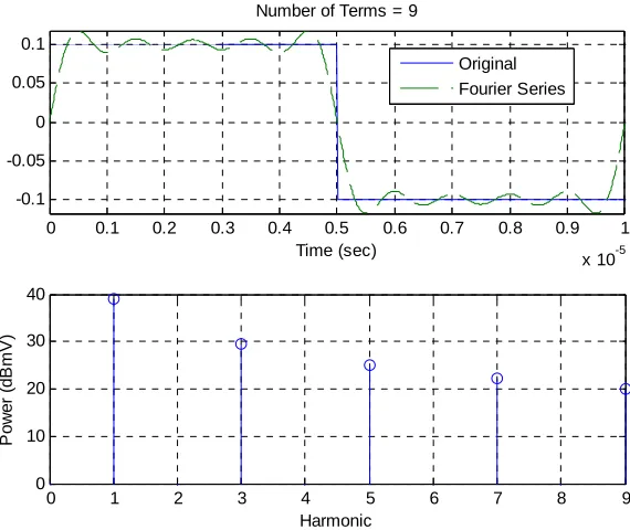
a) Plot the Fourier series representation and the single sided power spectrum in dBmV for each of the waveforms listed below. Use 9 terms for each function. It is probably easiest to use your program Complex_Fourier_Series.m. You should use the log10 command to compute the base 10 logarithm. You should also use the

subplot command so you can plot both a signal and its Fourier series representation in one graph, and its single-sided power spectrum in a subsequent graph within the same window. Utilize the stem command in Matlab to do the plotting. For the power spectrum plot, the y-axis should be labeled Power(dBmV), the x-axis labeled

Harmonic .Your plots for function x t₂( ) should look like those in Figure 1. (Note the axis on the top graph is limited using the command axis(‘tight’), and is limited on the second plot using the command axis([0 N 0 40]); )

The waveforms, each having zero DC offset, are:

i) x t1

( )

=0.1cos 2 100 10

(

π × 3t

)

V

II) x2

( )

t is a square wave of period 10 μs and peak-to-peak amplitude 0.2 V.

III) x t3

( )

is a triangle wave of period 10 μs and peak-to-peak amplitude 0.2 V.

Just to be sure there is no confusion regarding the waveforms, they are displayed below.

i) ii)

0 0.1 0.2 0.3 0.4 0.5 0.6 0.7 0.8 0.9 1

x 10-5 -0.1

-0.05 0 0.05 0.1

Time (sec) Number of Terms = 9

Original Fourier Series

0 1 2 3 4 5 6 7 8 9

0 10 20 30 40

Harmonic

Po

w

e

r (

d

Bm

V)

[image:4.612.159.444.71.311.2]

Figure 1: Results for problem 8a for functionx t2( ).

b) For each waveform, create a table containing a column of values of and a column of values of predicted decibel levels (dBmV). Do not read these from your plots, but get them directly from you program. Note that if you do not put a semicolon after a statement in Matlab, the values in the array will be printed to the screen.

k

c

c) If the periodic signal is a pulse train, we know that the magnitude of the coefficients will be given by

|c_k| A sinc k

T T

τ ⎛ τ ⎞

= _{⎜ ⎟}

⎝ ⎠

whereA is the amplitude of the pulse, τ is the duration of the pulse, and T is the

period. The ratio

T τ

is the duty cycle of the pulse. Using this expression, and our

knowledge of the properties of the sinc function, we can determine that the will be

zero whenever

k

c

1, 2, 3,... k

T τ ₌

or whenever k T , 2T, 3T ,...

τ τ τ

= These zeros, or nulls, will

occur at frequencies k _o k2 2 ,4 ,6 ,... T

π π π π

ω

τ τ τ

= =

In order to help see what is happening, in the following three problems we will fix the axes so they always plot over the same range of frequencies. Use the axis

command to limit the frequencies from 0 to radians/sec and the power from 0 to 40 dBmV.

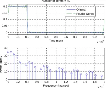
i) We will first look at the case of a fixed length period with a changing pulse width. We will assume the pulse has an amplitude of 0.2 V with a fixed period of T=10μs . Mathematically our pulse is defined as

0.2 0 ( )

0

t x t

t T τ τ

≤ ≤ ⎧

= ⎨ _{< <}

⎩

Plot the Fourier series representation of x t( )and the single sided power spectrum for

2 s

τ = μ , τ =1μs, and τ =0.5μs. Figure 2 shows how your plot should look (to get the

τ to display, use \tau in the title). Use 40 terms in the Fourier series representation. Do the locations of the nulls occur where you expect them to occur? Does the spacing between spectral components change as the pulse width (τ ) changes?

0 0.1 0.2 0.3 0.4 0.5 0.6 0.7 0.8 0.9 1 x 10-5 0

0.05 0.1 0.15 0.2

Time (sec) Number of Terms = 40

Original Fourier Series

0 0.2 0.4 0.6 0.8 1 1.2 1.4 1.6 1.8 2 x 107 0

10 20 30 40

Frequency (rad/sec)

Po

w

e

r (

d

Bm

[image:5.612.123.482.258.561.2]

V)

Figure 2: Plot for 8c-(i), Amplitude = 0.2V, τ =2μs, and T =10μs.

ii) Now we will look at the case of a fixed pulse length with a varying period. We will assume the pulse has an amplitude of 0.2 V with a fixed pulse width of τ =2μs. Plot the Fourier series representation of x t( )and the single sided power spectrum for

10

T = μs, T =20μs, and T =40μs. Use 120 terms in the Fourier series

iii) Now we will look at the case of a fixed duty cycle with a varying period and pulse width. We will assume the pulse has an amplitude of 0.2 V and a fixed duty cycle of 20%. Plot the Fourier series representation of x t( )and the single sided power

spectrum for (τ =1μs T, =5μs), (τ =2μs T, =10μs), and (τ =4μs T, =20μs). Use 120 terms in the Fourier series representation. Do the locations of the nulls occur where you expect them to occur? Does the spacing between spectral components change as the period (T) changes?

Appendix

There are a number of different ways of graphically presenting the information in the Fourier series representation of a periodic function. The most common methods of presenting this information are by plotting the spectrum of the signal, or the power spectrum of the signal. In the following examples we will use the function

0 2

( ) 1 1

1 1 2

t

f t t t

t

1

− ≤ < − ⎧

⎪

=_⎨ − ≤ < ⎪ _{≤ <} ⎩

Spectrum of a Periodic Signal The spectrum of a periodic signal is a plot of the

magnitude |c_k | against the corresponding frequencykω_o, and the phase against the corresponding frequency. Since our signal is periodic we only have values at

discrete frequencies (

k

c (

o

kω ), we do not know what happens in between these discrete frequencies so we do not “connect the dots”. Since ω_ois common to all of the

discrete frequencies, we often plot against the harmonic k, rather than the frequency

o

kω . Figure 3 shows the spectrum of f t( ).

Power Spectrum of a Periodic Signal The power spectrum of a signal tells us how

the power in the signal is distributed in frequency. To plot the power spectrum of a signal, we consider each term of the complex Fourier series, jk ot

k

c e ω . The average

power in this term is . The power spectrum indicates the power associated with each frequency, and is thus a plot of against frequency

2 |c_k |

2

|c_k | kω_o or just the

harmonic k. In this plot we need to include both positive and negative frequencies. Figure 4 shows the power spectrum of f t( ).

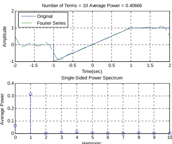
Single-Sided Power Spectrum of a Periodic Signal Because the magnitudes of

the coefficients are even (| | ), the powers associated with negative

frequencies are the same as those associated with positive frequencies. Since only positive frequencies are realizable, we often just want to plot the power against

|

k

2 2 2

0 1 2

|c | 2 |c | 2 |c | ... 2 |c_N |2

0

versus the corresponding frequency

0 0

0 ω 2ω ... Nω . Since the fundamental frequency ω₀is common to all of the

frequency terms, we often just plot against the harmonics . Figure 5

shows the single sided power spectrum of

0 1 2 ... N

( ) f t .

Spectrum Analyzer (SA) Display The SA displays a one-sided spectrum, but

instead of showing the value of 2c_k2 at each frequency, the spectrum analyzer shows average power in decibels with respect to a one millivolt RMS reference. For the sinusoid at frequency kf₀, the average power in decibels is given by

10

10 log k

k dB

ref

P P

P

= ,

where the power Pk represents the power spectrum coefficient

2

2c_k , and the power

Pref is the average power delivered to a one-ohm resistor by a one millivolt RMS

sinusoid. We have

(

)

2

10 2

2

10 log dBmV

0.001

k k dBmV

c

P = ⎛⎜ ⎞⎟

⎜ ⎟

⎝ ⎠

.

The units “dBmV” indicate that the reference for the decibels is a one millivolt RMSsinusoid.

-2 -1.5 -1 -0.5 0 0.5 1 1.5 2

-1 0 1 2

Time(sec)

A

m

p

lit

u

d

e

Number of Terms = 10 Average Power = 0.40666

Original Fourier Series

-10 -8 -6 -4 -2 0 2 4 6 8 10

0 0.2 0.4

Harmonic

A

m

pl

it

ude

Amplitude Spectrum

-10 -8 -6 -4 -2 0 2 4 6 8 10

-200 0 200

Harmonic

P

has

e

(

deg

rees

)

Figure 3: The spectrum of f t( ).

-2 -1.5 -1 -0.5 0 0.5 1 1.5 2

-1 0 1 2

Time(sec)

A

m

p

lit

u

d

e

Number of Terms = 10 Average Power = 0.40666

Original Fourier Series

-10 -8 -6 -4 -2 0 2 4 6 8 10

0 0.05 0.1 0.15 0.2

Harmonic

A

v

erage P

ower

Power Spectrum

[image:8.612.152.447.83.340.2]

Figure 4: The power spectrum of f t( ).

-2 -1.5 -1 -0.5 0 0.5 1 1.5 2

-1 0 1 2

Time(sec)

A

m

pl

it

ude

Number of Terms = 10 Average Power = 0.40666

Original Fourier Series

0 1 2 3 4 5 6 7 8 9 10

0 0.1 0.2 0.3 0.4

Harmonic

A

v

e

rage P

ow

er

Single-Sided Power Spectrum

[image:8.612.156.446.393.635.2]