ECE-205 Dynamical Systems

ECE-205

Dynamical

Systems

Course Notes

Fall 2013

Chapter 1: Electrical Systems Page 3

1.0 Electrical Systems

The types of dynamical systems we will be studying can be modeled in terms of algebraic equations, differential equations, or integral equations. We will begin by looking at familiar mathematical models of ideal resistors, ideal capacitors, ideal inductors, and ideal op amps. Then we will begin putting these models together to develop models for RL and RC circuits. Finally, we will review solution techniques for the first order differential equation we derive to model the systems.

1.1 Ideal Resistors

The governing equation for a resistor with resistanceR is given by Ohm’s law, ( ) ( )

v t =Ri t

where v t( ) is the voltage across the resistor and i t( ) is the current through the resistor. HereRis measured in Ohms,v t( )is measured in volts, andi t( ) is measured in amps. The entire expression must be in volts, so we get the unit expression

[volts] = [Ohms][amps]

1.2 Ideal Capacitors

The governing equation for a capacitor with capacitance C is given by ( )

( ) dv t

i t C

dt =

HereCis measured in farads, and again v t( ) is measured in volts and i t( )is measured in amps. This expression also helps us with the units. The entire expression must be in terms of current , so looking at the differential relationship we can determine the unit expression

[amps] = [farads][volts]/[seconds]

We can integrate this equation from an initial time t₀ up to the current time t as follows: ( )

( ) dv t

i t C

dt =

1

( ) ( )

i t dt dv t

C =

Chapter 1: Electrical Systems Page 4 dummy variableλ. Also we incorporate the fact that at time t₀ the voltage is v t( )₀ , while at time

t the voltage is v t( )

0

) ) ( ( 1

( ) ( )

o

v t t

t v t

i d dv

C

∫

∫

Carrying out the integration we get

0

0 1

)

( ) ( ) (

t t

i d v t v t C

∫

0 0

1 )

( ) ( ( )

t t

v t v t i

C λ λd +

=

∫

This expression tells us there are two components to the voltage across a capacitor, the initial voltage v t( )₀ and the part due to any current flowing through the capacitor after that time,

0 1

( ) t t

i d C

∫

Finally, these expressions help us determine some important characteristics of our ideal capacitor:

• If the voltage across the capacitor is constant, then the current through the capacitor must be zero since the current is proportional to the rate of change of the voltage. Hence, a capacitor is an open circuit to dc.

• It is not possible to change the voltage across a capacitor in zero time .The voltage across a capacitor must be a continuous function of time, otherwise an infinite amount of current would be required.

1.3 Ideal Inductors

The governing equation for an inductor with inductance L is given by ( )

( ) di t

v t L

dt =

HereL is measured in henrys, and again v t( ) is measured in volts andi t( ) is measured in amps. This expression also helps us with the units. The entire expression must be in terms of voltage , so looking at the differential relationship we can determine the unit expression

[volts] = [henrys][amps]/[seconds]

Chapter 1: Electrical Systems Page 5 ( )

( ) di t

v t L

dt =

1

( ) ( )

v t dt di t

L =

Next, since we want to integrate up to a final time t, so we again have chosen to use the dummy variableλ. Also we incorporate the fact that at time t₀ the current is,i t( )₀ while at time t the current is i t( ).

0

) ) ( ( 1

( ) ( )

o

i t t

t i t

v d di

L

∫

∫

0

0 1

)

( ) ( ) (

t t

v d i t i t L

∫

0 0

1 )

( ) ( ( )

t t

i t i t v

L λ λd +

=

∫

This expression tells us there are two components to the current through an inductor, the initial current i t( )₀ and the part due to any voltage across the inductor after that time,

0 1

( ) t t

v d

L

∫

• If the current thought an inductor is constant, then the voltage across the inductor must be zero since the voltage is proportional to the rate of change of the current. Hence, an inductor is a short circuit to dc.

• It is not possible to change the current through an inductor in zero time .The current through an inductor must be a continuous function of time, otherwise an infinite amount of voltage would be required.

1.4 Ideal Op Amps

In this class we will assume only ideal op amps. For these op amps we only need to remember the following rules:

• There is no current flowing into the op amp

Chapter 1: Electrical Systems Page 6

Example 1.4.1 Consider the op amp circuit show in Figure 1.1.

Figure 1.1. Op amp circuit for Example 1.4.1.

Summing the currents flowing into the negative terminal of the op amp, v t−( ), we can write

( ) ( ) ( ) ( )

0

in out

a b

v t v t v t v t

R R

− −

− ₊ − ₌

At the positive terminal of the op amp,v t+( ), we have v t+( )=0. Since the positive and negative input terminals of an ideal op amp are at the same voltage we have v t+( )=v t−( )=0 and then

( ) b ( )

out in

a

R

v t v t

R = −

Example 1.4.2. Consider the op amp circuit shown in Figure 1.2.

Figure 1.2. Op amp circuits for Example 1.4.2.

Chapter 1: Electrical Systems Page 7

( ) ( )

( ) ( )

b in a b

d out c d

R

v t v t

R R

R

v t v t

R R

+

−

= +

= +

Since the positive and negative input terminals of an ideal op amp are at the same voltage we have v t+( )=v t−( ) and then

( ) ( )

b d

in out

a b c d

R R

v t v t

R +R = R +R

or

( ) b c d (t)

out in

a b d

R R R

v t v

R R R

+ =

Chapter 1: Problems Page 8

Chapter 1 Problems

1.1) For the following circuit, show that ( ) b d ( )

out in

a c R R

v t v t

R R

 

=  

 

1.2) For the following circuit, show that ( ) e b ( )

out in

d a b

R R

v t v t

R R R

 

= −_{ }

+

 

1.3) For the following circuit, show that ( ) b c d ( )

out in

a d

R R R

v t v t

R R

 + 

= −_{ }

 

Chapter 1: Problems Page 9

1.4) For the following op-amp circuits we can write v_out( )t =Gv t_in( ). Determine and expression for G.

Answers: , ,

g f f

d b c d b

c g a b e c a b

R R R

R R R R R

G G

R R R R R

G

R R R

+ −

− +

= =

+ +

Chapter 2: First Order Circuits Page 11

2.0 First Order Circuits

A first order circuit is a circuit with one effective energy storage element, either an inductor or a capacitor. (In some circuits it may be possible to combine multiple capacitors or inductors into one equivalent capacitor or inductor.) We begin this section with the derivation of the governing differential equation for various first order circuits. We will then put the first order equation into a standard form that allows us to easily determine physical characteristics of the circuit. Next we show an alternative method for checking some parts of the governing differential equations. We then solve the differential equations for the case of piecewise constant inputs, and finish the section with an alternative method of solving the differential equations using integrating factors.

2.1 Governing Differential Equations for First Order Circuits

In this section we derive the governing differential equations that model various RL and RC circuits. We then put the governing first order differential equations into a standard form, which allows us to read off descriptive information about the system very easily. The standard form we will use is

( )

( ) ( )

dy t

y t Kx t

dt

τ + =

Here we assume the system input isx t( ) and the system output isy t( ). τ is the system time constant, which indicates how long it will take the system to reach steady state for a step (constant) input. K is the static gain of the system. For a constant input of amplitudeA (x t( )= Au t( ), where u t( ) is the unit step function), in steady state we have dy t( ) 0

dt = and

( ) ( )

y t =Kx t =KA. Hence the static gain lets us easily compute the steady state value of the output. For circuits with capacitors the differential equation will in general be in terms of a voltage (the output y t( )will be a voltage), while for circuits with inductors the differential equation will in general be in terms of current (the outputy t( )will be a current) .

Example 2.1.1. Consider the RC circuit shown in Figure 2.1.

Figure 2.1. Circuit for Example 2.1.1.

R

C

+

-

+

Chapter 2: First Order Circuits Page 12 The voltage source is v t_s( ). We start to derive the governing differential equation by determining

the single current in the loop

( ) ( ) ( )

( ) s c ( ) c

R C

v dv

i i

R

t v t t

t t C

dt −

= = =

or

( ) ( ) ( ) c t s c

dv v

C dt

v R

t − t

=

wherev t_c( ) is the voltage across the capacitor and the current in the loop is equal to the current through the resistor ( )i t_R and the current through the capacitor i t_C( ). We can put this into a more standard form by rearranging the terms

( )

( ) ( ) c

c s

dv

RC t v t v t

dt + =

If we define the time constantτ =RC, then we have ( )

( ) ( ) c

c s

dv v t

t v t

dt

τ + =

Here the static gainK =1.

Example 2.1.2. Consider the RC circuit shown in Figure 2.2.

Figure 2.2. Circuit used in Example 2.1.2.

Again the voltage source is v t_s( ). We again start to derive the governing differential equation by determining the current through resistorR_a,

( ) ( ) s c( )

a

v

i t v

R

t − t

=

R

C

+ -

+

-

Chapter 2: First Order Circuits Page 13 This current must be equal to the sum of the currents through the capacitor and R_b,

(

( ) c ) ( ) b c v dv i C d t R t t

t = +

Equating these we get the governing differential equation: ( ) ( ) ( ) (

( ) s c c c )

a b

v v dv

i t C

R t v d t R t t t = − = +

Rearranging terms we get

1 1

( ) 1

( ) ( ) c s a b c a dv

C v v

dt R R R

t t t   +_ + _   = 1 ( ) ( ) ( ) a b s a b c c a t R t dv R

C v v

dt + R R R t

+ ₌

or

( )

( ) ( )

a b b

s a b c a b c R dv v v R d

R C t

t

R

t t

R + = R R

+ +

With time constant a b a b R C R R R τ =

+ and static gain

b a b

R K

R +R

= we get

( ) ( ) ( ) c c s t dv v v

dt t K t

τ + =

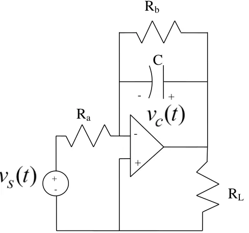
Example 2.1.3. Consider the operational-amplifier circuit shown in Figure 2.3.

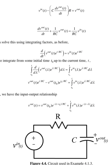
Chapter 2: First Order Circuits Page 14 The input voltage is againv t_s( ) and the output voltage (the voltage across the load resistorR_L) is the same as the voltage across the capacitor (since the + terminal of the op amp is assumed to be grounded). We will assume an ideal op amp, which implies the conditions

( ) ( ) 0 ( ) ( ) i t i t

v t v t

+ −

+ −

= =

=

Let’s look at the currents flowing into the negative (feedback) terminal of the op-amp using the ideal op-amp model. Since for our example the non-inverting terminal is tied to ground we have

( ) 0

v t+ = . With these assumptions our governing differential equation becomes ( ) ( ) ( )

0 s c c

a b

v t v t dv t

C

R R dt

= + +

Rearranging this gives

( ) ( ) _s( )

b a

c c

dv t v t v t

C

dt + R = − R

or

( )

( ) b ( )

b s

c c

a

dv t R

R C v t v t

dt + = −R

Setting the time constant τ =R C_b and static gain b a

R K

R

= − we finally have

( )

( ) ( ) c

c s

dv t

v t Kv t

dt

τ + =

Example 2.1.4. Consider the RL circuit shown in Figure 2.4.

Figure 2.4. Circuit for Example 2.1.4..

The single current in the loop is given by

( ) ( ) ( ) v ts v tL

i t

Chapter 2: First Order Circuits Page 15 where

(

( ) )

L

d

L i t

v

t t

d =

Combining and rearranging we get

( ) ( )

( ) s

di t

L Ri t v

dt + = t

or

( ) 1

( ) s( )

L di t

i t v

R dt + = R t

With time constant L

R

τ = and static gain K 1 R

= the governing differential equation is ( )

( ) s( )

di t

i t Kv

dt t

τ + =

Example 2.1.5. Consider the RC circuit shown in Figure 2.5. The single current source must be

divided between the current flowing through resistor R_b and the current flowing through the capacitorC,

( ) ( )

( ) c c

s

b

v dv

i t C

R t

t t

d

= +

Rearranging we get

( )

( ) ( ) c

b c b s

dv

RC t v t R i

dt + = t

With time constantτ =R_bC and static gain K =R_b the governing differential equation is ( )

( ) ( ) c

c s

t dv

v

dt t Ki t

τ + =

Figure 2.5. Circuit used in Example 2.1.5.

R

C

+

-

Chapter 2: First Order Circuits Page 16

2.2 Thevenin Resistance, Time Constants, and Static Gain

Although we are focusing our attention on deriving the governing equations for first order circuits, it is useful and very convenient to be able to check our equations as much as possible. First of all, for first order RC circuits the time constants will be of the formτ =R C_{th eq} whereR_th is the Thevenin resistance seen from the ports of the equivalent capacitor, C_eq. For first order RL circuits the time constants will be of the form eq

th L

R

τ = whereR_th is the Thevenin resistance seen from the ports of the equivalent inductor, L_eq. Recall that when determining the Thevenin

resistance all independent voltage sources are treated as short circuits, and all independent current sources are treated as open circuits.

Secondly, if we are looking at constant inputs, then we use the fact that a capacitor is an open circuit to dc and an inductor is a short circuit to dc. In addition, for constant inputs in steady state all of the time derivatives are zero (in steady state nothing changes in time).

Example 2.2.1. Consider the circuit shown in Figure 2.1 (Example 2.1.1). The Thevenin

resistance seen from the capacitor is equal toR, so the time constant is τ =RC. For a dc input, the capacitor looks like an open circuit, so in steady state the voltage across the capacitor is equal to v_s, the input voltage, so the static gain is K =1. These results match our previous results.

Example 2.2.2. Consider the circuit shown in Figure 2.2 (Example 2.1.2). The Thevenin

resistance seen from the capacitor is || a b th a b

a b

R R

R R

R R

R

= =

+ , so the time constant is

a b th

a b

R R R

C R C

R

τ = =

+ . For a dc input, the capacitor looks like an open circuit, so in steady state the

voltage across the capacitor is given by the voltage divider relationship b

c s

a b

R

v v

R R

=

+ , so the

static gain is b a b

R K

R +R

= . These results match our previous results.

Example 2.2.3. Consider the circuit shown in Figure 2.3 (Example 2.1.3). The Thevenin

resistance seen by the capacitor is a little more difficult to determine, and to do it correctly is beyond the scope of this course. For a dc input, the capacitor looks like an open circuit, so summing the currents into the negative terminal of the op amp we have c s 0

b a

v v

R + R = , or in steady

state b

c s

a

R

v v

R

= − Hence the static gain is b a

R K

Chapter 2: First Order Circuits Page 17

Example 2.2.4. Consider the circuit shown in Figure 2.4 (Example 2.1.4). The Thevenin

resistance seen by the inductor is R_th =R. For a dc input, the inductor looks like a short circuit. Hence the steady state current flowing in the circuit for a dc input is i 1 v_s

R

= , so the static gain is 1

K R = .

Example 2.2.5. Consider the circuit shown in Figure 2.5 (Example 2.1.5). The Thevenin

resistance seen by the capacitor is R_th =R_b so the time constant is τ =R C_b . For a dc input the capacitor looks like an open circuit, so in steady state v_c=R i_b , so the static gain is K =R_b.

2.3 Solving First Order Differential Equations

In this section we will go over two methods for solving first order differential equations. We will initially solve the equations by breaking the solution into the natural response (the response with no input) and then the forced response (the response when the input is turned on). We will apply this method to problems where the input is a constant value, or is switched between constant values. This method will also work with any input, and we will examine the results for a sinusoidal input later. In the last section we will go over a different method of solution using integrating factors, which will work for any type of input, and is an important method in helping us characterize how a system will respond to any type of input.

2.3.1 Solution using Natural and Forced Responses

Consider a system described by the first order differential equation ( )

( ) ( )

dy t

y t Kx t

dt

τ + =

In this equation, τ is the time constant and K is the static gain. We will solve this equation in two parts. We will first determine the natural response,y t_n( ). The natural response is the when the input is zero. Then we will determine the forced response,y t_f( ). The forced response is the response due to the input only. The total response is then the sum of the natural and forced responses, y t( )= y tn( )+y tf( ).

Natural Response: To determine the natural response we assume there is no input in the system, so we have the equation

( )

( ) 0 n

n

dy t

y t dt

τ + =

Let’s assume a solution of the formy tn( )=c ert, wherec and rare parameters to be determined. Substituting this assumption into the differential equation we get

[ 1] 0

rt rt rt

rce ce ce r

Chapter 2: First Order Circuits Page 18 Ifc=0 then we are done, and the natural response will bey t_n( )=0. This solution certainly satisfies the differential equation. However, ifc≠0, and since ert can never be zero, we must haveτr+ =1 0, or r 1

τ

= − . In this case the natural response will be /

( ) t n

y t =ce− τ.

Forced Response: To determine the forced response we must know the system input, x t( ). We will initially assume an input that is zero before t=0 and then has constant amplitude A for

0 t≥ ,

0 0

( )

0 t x t

A t < ≥  =   Then for t≥0 we have the equation

( )

( ) f

f dy t

y t KA dt

τ + =

Since this is a linear ordinary differential equation we only need to find one solution. One obvious solution to this equation is the solution in steady state, when dy tf( ) 0

dt = . In steady state we have

( ) f

y t =KA

Note that for a constant input, the steady state output is the product of the static gain and the amplitude of the input.

Total Solution: The total solution to the problem is the sum of these two solutions

/ ( ) _n( ) _f( ) t

y t =y t +y t =ce− τ +KA

Now assume the initial time is t₀ and at this time the output is denoted y t( )₀ . Substituting this into our equation we have 0/

0

( ) t

y t =ce− τ +KA, or

(

)

( ) t

c= y t −KA e τ, and our total solution is

0 ( )/ 0

( ) ( ( ) ) t t

y t = y t −KA e− − τ +KA

For simplicity, let’s write our steady state value explicitly, soy( )∞ =KA and we have the solution

0 ( )/ 0

( ) ( ( ) ( )) t t ( )

y t = y t − ∞y e− − τ +y ∞

Significance of the Time Constant

Chapter 2: First Order Circuits Page 19 rest (y(0)=0) and the final value is one (y( )∞ =1). Let’s look at the response of our system as the time t takes on the values of integer number of time constants:

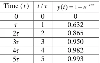
Time (t) t/τ /

( ) 1 t y t = −e− τ

0 0 0

τ 1 0.632

2τ 2 0.865

3τ 3 0.950

4τ 4 0.982

5τ 5 0.993

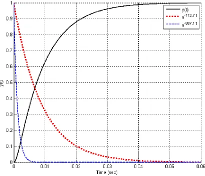
Figure 2.6 show this result graphically, The way this information is usually interpreted is that a system is within 5% of its final value in 3 time constants, within 2% of its final value in 4 time constants, and within 1% of its final value in 5 time constants. Hence the use of time constants gives us a quick way to describe one aspect of the behavior of a system. As we will see, as the systems become more complex, the use of time constants indicates which part of the solution is the most important and how the system responds to periodic inputs (sines and cosines).

Figure 2.6. Graph of y t( )= −1 e−t/τ for t=0τ up to t=7τ. y t( ) is within 5% of its final value in 3 time constant, within 2% of its final value in 4 time constants, and within 1% of its final value in 5 time constants.

0 1 2 3 4 5 6 7

0 0.1 0.2 0.3 0.4 0.5 0.6 0.7 0.8 0.9 1

Number of Time Constants

y

(t

Chapter 2: First Order Circuits Page 20

Example 2.3.1. Consider the circuit in Figure 2.2 (Example 2.1.2). Let’s first assume 2

a Rb

R = = kΩand C=1µF. Then R_th= Ω1k , τ =1ms, and K =0.5. Next we will assume the initial voltage on the capacitor is zero (v t_c( )₀ =v_c(0)=0) and the input is as follows:

0 0

2 0

2 8

8

1 16

( )

16 s

t

v

t

t t

t = ≤ ≤

≤ < 

 

− < 

 _> 

Here the input is in volts and the time is measured in milliseconds. We now want to determine the output. We will do this by looking at the initial and final values for each time interval, where the time intervals are determined by the times during which the input voltage is constant. The differential equation is

( )

( ) ( ) c

c s

dv t

v t Kv t

dt

τ + =

Clearly ( )y t =v t_c( ) and ( )x t =v t_s( ). The solution in each interval will be of the form

[

]

0

( ) ( ) ( ) t t ( )

y t = y t − ∞y e− − τ + ∞y

At this point we just need to be able to determine what y t( )0 and y( )∞ mean for each interval. First interval (0≤ <t 8 ms) : We have the initial value in this interval (0)y =v_c(0)=0 volts. To determine the final value, we use the static gain and the amplitude of the input for this interval.

1

( ) ( ) 2 2 1

2 c

v ∞ = ∞ =y K =  =

Hence for this interval, we have the solution

/ /0.001 ( ) ( ) t 1 1 t c

v t = y t = −e− τ + = −e−

Before we go on to the next interval we need to figure out the value of y t( ) at the end of this interval, this value will be the initial point during the next interval. At the end of the interval we will have

0.008/0.001 8 1

(0.008) 1 e 0.99966 1.0

y = −e− = − − = ≈

Second interval (8< ≤t 16 ms) : The initial value for this interval will be the end point of the previous interval, so y t( ) 1₀ = . To determine the final value we again use the static gain

1

( ) ( 2) ( 2) 1 2

K

y ∞ =  − =  − = −

Chapter 2: First Order Circuits Page 21 the time at the beginning of the interval from our actual time in our form of the solution, so our time will be measured from the beginning of the interval. Our solution for this interval is then

( 0.008)/ ( 0.008)/0.001

( ) [1 ( 1)] t ( 1) 2 t 1

y t = − − e− − τ + − = e− − − At the end of this interval we will have

(0.016 0.008)/0.001 8

2 1 2 1 0.999

(0.016) e e 33 1.0

y = − − − = − − = − ≈ −

Third interval (t>16 ms) : The initial value for this interval will be the end point of the previous interval, so y t( )₀ = −1. To determine the final value we have

1 ( ) 1

2

y ∞ =K =K =

Again we must scale our solution so time is measured from the beginning of the interval, so we have

( 0.016)/ ( 0.016)/0.001 0.

( ) [ 1 0.5] t 5 1.5e t 0.5

y t = − − e− − τ + = − − − +

Total solution: To get the total solution, we list the solutions during each time interval: /0.001

( 0.008)/0.001 ( 0.016)/0.001

1 8

( )

2 1 16

0 0

0 ( )

8

1.5 0.5 16

t

c t

t

e t ms

t

e t m

t v s y t e t ms − − − − − 

 _{− ≤ <}

 = _ − < = + ≤ <  − ≥ 

To get the current through the capacitor, we use the relationship ( ) c( ) c

dv t

i t C

dt

= for each time interval above. Doing this we get

/0.001 ( 0.008)/0.001 ( 0.016)/0.001 0 0 0 8 0.001 8 ( ) ( ) 0.002 16 0.015 16 t c c t t

e t ms

dv t

t C

e t m

t s dt i t e ms − − − − − 

 _{≤ <}

 = _ ≤ <  − ≥  < =

Here ( )i t_c is measured in amps.

Chapter 2: First Order Circuits Page 22 was held constant for an equivalent of eight time constants, so the voltage across the capacitor had essentially reached steady state.

Finally is useful to point out that if the voltage across the capacitor is described by the relationship

/

( ) [ (0) ( )] t ( ) c t vc vc e vc

v = − ∞ − τ + ∞

Then the current through the capacitor is given by

/ ( )

( ) c [ (0) ( )] t

c c c

t

t Cdv C v v e

i

dt

τ

τ − ∞ −

= − =

What this means is that if the voltage across a capacitor is growing exponentially, then the current through the capacitor is decreasing exponentially. Similarly, if the voltage across a capacitor is decreasing exponentially, the current through the capacitor will be growing exponentially. This is also behavior our results show. Similar results also hold for inductors.

Example 2.3.2. Consider the circuit in Figure 2.4 (Example 2.1.4). Let’s first assume 100

th

R=R = ΩandL=10mH. Then 0.01 0.0001 100 100

L

s R

τ = = = = µ andK=0.01. Next we will assume the initial current through the inductor is i(0)=10mAand the input is as follows:

0 0

2 0 0.1

( )

3 0.1 0.25

4 0.25

s

t

t v t

t

t < 

 _{≤ <} 

= _{− ≤ <} 

 _≥



Here the input is in volts and the time is measured in milliseconds. We now want to determine the output. We will do this by looking at the initial and final values for each time interval, where the time intervals are determined by the times during which the input voltage is constant. The differential equation for this system is again

( )

( ) s( )

di t

i t Kv t

dt

τ + =

Clearly y t( )=i t( ) and ( )x t =v ts( ). The solution in each interval will be of the form

[

]

0

( ) ( ) ( ) t t ( )

y t = y t − ∞y e− − τ + ∞y

Chapter 2: First Order Circuits Page 23

Figure 2.7. Results for Example 2.3.1.

First interval (0≤ <t 0.1ms) : We have the initial value y(0)=i(0)=0.01amps in this interval. To determine the final value, we use the static gain and the amplitude of the input for this interval

1

( ) ( ) 2 2 0.02

100

i ∞ = ∞ =y K =  =

Hence for this interval, we have the solution

[

]

( ) (0) ( ) t ( ) [0.01 0.02] t 0.02 0.01 t 0.02

y t = y − ∞y e− τ + ∞ =y − e− τ + = − e− +

Before we go on to the next interval we need to figure out the value of y t( ) at the end of this interval, this value will be the initial point during the next interval. At the end of the interval we will have

0.0001/0.0001 1

(0.0001) 0.01 0.02 0.01 0.02 0.01632

y = − e− + = − e− + =

0 5 10 15 20 25

-2 -1 0 1 2

V s

(t

) (v

o

lt

s

)

0 5 10 15 20 25

-1 -0.5 0 0.5 1

V c

(t

) (v

o

lt

s

)

0 5 10 15 20 25

-2 -1 0 1 2

i c

(t

) (m

A

)

Chapter 2: First Order Circuits Page 24 Third interval (0.1≤ <t 0.25ms) : The initial value for this interval will be the end point of the previous interval, soy t( )₀ =0.01632. To determine the final value we again use the static gain

) 3) 0.01

( K ( ( 3) 0.03

y ∞ =  − =  − =−

We again need to subtract the time at the beginning of the interval from our actual time in our form of the solution, so our time will be measured from the beginning of the interval. Our solution for this interval is then

( 0.0001)/ ( 0.0001)/0.0001

( 0.03) 0.04632 0.03

( ) [0.01632 ( 0.03)] t e t

y t = − − e− − τ + − = − − −

At the end of this interval we will have

(0.00025 0.0001)/0.0001 1.5

0.04632 0.03 0.04632

(0.00025) e e 0.03 0.01966

y = − − − = − − = −

Fourth interval (t≥0.25ms) : The initial value for this interval will be the end point of the previous interval, soy t( )₀ = −0.01966. To determine the final value we have

( ) 4 0.04

y ∞ =K =

Again we must scale our solution so time is measured from the beginning of the interval, so we have

( 0.0025)/ ( 0.00025)/0.0001 0.

( ) [ 0.01966 0.04] t 04 0.05966 t 0.04

y t = − − e− − τ + = − e− − +

Total solution: To get the total solution, we list the solutions during each time interval:

/0.0001 ( 0.0001)/0.0001

( 0.00025)/0.0001

0.01 0.02 0.1

( )

0.04632 0.03 0.1

0 0 0 0.25 0.05966 0.25 ( ) 0.04 t L t t t

e t ms

t e i y t ms ms t t e − − − − − 

 _{− + ≤ <}



= _

− ≤ < 

− + ≥



< =

To get the voltage across the inductor we use the relationship ( ) L( ) L di v L t t t d

= and compute the voltage for each time interval. Doing this we get

/0.0001 ( 0.0001)/0.0001 ( 0.00025)/0.0001 0.1 ( ) ( ) 4.632 0.1 0 0.25 5.966 0 0 0.25 t L L t t t

v e t m

t

s di t

t L

e t ms

dt e ms − − − − − 

 _{≤ <}

 = _− ≤ < ≥ < =  

Chapter 2: First Order Circuits Page 25 be, while in this case the voltage across the inductor is not continuous. Again let’s look at our solution to see if it makes sense. First of all, the voltage/current relationships for the inductor are consistent with what we expect. The initial current in the inductor is 10 mA, as we require, and the initial voltage from the source is 2 volts. Applying Kirchhoff’s laws around the loop, we expect the initial voltage drop across the inductor to be given by

(0) (0) 2 (0.01)(100) 1 s i R

v − = − = volts, which is what we have. In steady state the inductor looks like a short circuit, so there should be no voltage drop across the inductor once the system

reaches steady state, which again matches our results. Note that the system only reaches steady state near 0.7 or 0.8 ms. In addition, in steady state the voltage drop across the resistor must match the voltage supplied by the source, or v_s( )∞ − ∞i( )R= −4 (0.04)(100)=0volts, which again matches our results. Let’s look at the results at one other convenient point in time, say

0.2

t= ms. Using the equations we derived above (and the known input) we have (0.0002) 3

(0.0002) 12.96 (0.0002) 1.70

s l L

v volts

i mA

v volts

= − = −

= − Applying Kirchhoff’s laws around the loop we have

(0.0002) (0.0002) (0.0002) 3 ( 0.01296)(100) ( 1.70) 0.0

s s L

v −i R v− = − − − − − ≈

We can obviously check as many points in time as we want in this way. This type of checking does not guarantee our answer is correct, but it does help find obvious errors.

2.3.2 Solution Using Integrating Factors

An alternative method of solution of first order differential equations is by the use of integrating factors. This method of solution is important to understand because as we start to analyze different types of systems, we need to be able to understand how we would solve for the output when we don’t actually know what the input is. This helps us characterize systems independent of the actual (specific) input.

The use of integrating factors for solving first order differential equations is based on the fact that when we differentiate an exponential, we get the same exponential back multiplied by some other term. For example, if x t( )=eφ( )t , then

( ) ( )

( ) t t ( ) ( ) ( )

d d d d

x t e x t

dt dt e dt dt

t t

φ ₌ φ φ φ

= =

In what follows, the method looks fairly lengthy, but with practice most of the steps can be done in your head. Let’s apply this idea to our equation

( )

( ) ( )

dy t

y t Kx t

dt

Chapter 2: First Order Circuits Page 26

Figure 2.8. Results for Example 2.3.2. This method will work better if we rearrange our equation a bit to the form

( ) 1

( ) ( )

dy t K

y t x t

dt +τ = τ

Next, we look at differentiating the product ( ) ( ) t

y t eφ , where φ( )t will be determined by the differential equation we are trying to solve. This leads to the equation

( ) ( ) ( ) ( ) ( ) ( ) ( )

( ) t t ( ) t t ( ) ( )

d dy t d dy t d

y t e e e e y t

dt dt d

t t

t t

t t d

y

d

φ φ φ φ φ  φ 

  =_ + = +

 _ _

Next, we equate the term in brackets to the left hand side of our original differential equation, 0 0.1 0.2 0.3 0.4 0.5 0.6 0.7 0.8

-4 -2 0 2 4

V s

(t

) (v

o

lt

s

)

0 0.1 0.2 0.3 0.4 0.5 0.6 0.7 0.8 -20

-10 0 10 20 30 40

iL

(t

) (m

A

)

0 0.1 0.2 0.3 0.4 0.5 0.6 0.7 0.8 -6

-4 -2 0 2 4 6 8

v L

(t

) (v

o

lt

s

)

Chapter 2: First Order Circuits Page 27

( ) ( ) ( ) 1

( ) ( )

dy t d dy t

y t y t

dt dt dt

t

φ

τ

+ = +

Clearly this means that

) 1 ( d d t t φ τ =

Solving this simple equation we get

( )t t

φ τ

=

Now we put this back into our equation above to get

/ / / /

( )

( ) 1 ( ) 1

( ) t t t t ( )

d dy t dy t

y t e e y e e y t

dt dt t dt

τ τ τ τ

τ τ

 

  = = +

  + _ _

The term on the far right is the same as the left hand side of our differential equation multiplied by t/

e τ, so this must equal the right hand side of our differential equation multiplied by the same thing,

/ / ( ) 1 /

( ) t t ( ) t ( )

d dy t K

y t e e y t e x t

dt dt

τ τ τ

τ τ

   

  = + =

  _ _ _ _

Next we eliminate the middle term to get the exact differential we want

/ /

( ) t t ( )

d K

y t e e x t

dt τ τ τ     =   _ _

Finally we integrate from and initial time t₀ with initial value y t( )₀ to final time t with value ( )

y t ,

0 0 / / ( ) ( ) t t t t K

e d e d

d x

d

y λ λ τ λ λ τ λ λ

λ   = τ

∫

∫

The left hand side can be integrated as

0 0 0 / / / / 0 ) ( ) ( ) ( ) ( t t t t t t K

e d y t e y t e x

d d

d

y λ λ τ λ τ e τ λ τ λ λ

λ  = − =

∫

∫

t

K

y t y t e τ e λ τ x λ λd τ

− − − −

= +

∫

Chapter 2: First Order Circuits Page 28

Example 2.3.1. Let’s now look at the same input as before, x t( )=A for t≥0 with initial condition t₀ =0 and y t( )₀ = y(0). The solution to the differential equation becomes

/ ( )/ 0 ( ) (0)

t

t t K

y t y e τ e λ τ Adλ

τ

− − −

= +

∫

/ / /

0 ( ) (0)

t

t t K

y t y e τ e τ eλ τ Adλ

τ

− −

= +

∫

/ / /

0

( ) (0) t t t

y t y e− τ e− τKA eλ τ λ_λ=

=

 

= + _{ }

/ / /

( ) y(0) t e t et 1

y t = e− τ + − τKA_ τ − _

/ /

) ) 1

( (0 t KA e t

y t =y e− τ + _ − − τ_

With the substitution y(∞ =) KA, we get

/ /

( ) (0) t y( ) 1 e t

y t = y e− τ + ∞ _ − − τ_

or

[

]

( ) (0) ( ) t ( )

y t = y − ∞y e− τ + ∞y the same solution as before.

Example 2.3.2. Let’s use integration factors to determine the solution to the differential equation

( )

( ) ( )

dy t

ay t bx t

dt = +

The first thing we need to do is put all of the y terms on the left hand side, ( )

( ) ( )

dy t

ay t bx t

dt − =

Then we need

( )

d

a d

t t

φ _{= −}

or

( )t at

φ = −

Then we have

( ) at at ( )

d

y t e e x t

dt b

− −

  =

 

Chapter 2: First Order Circuits Page 29 0 0 0 0 ( ) ( ) ( ) ( ) t t at

a at a

t t

d

e y d e y t e y t e bx d

d

λ _{λ λ} λ _{λ λ}

λ − − − −   = − =  

∫

∫

t

y t =e − y t +e

∫

Example 2.3.3. Let’s use integration factors to determine the solution to the differential equation

( )

( ) 2 ( )

dy t

ty t x t

dt − =

Then we need

( ) d t d t t

φ _{= −}

or 2 ( ) 2 t t φ = − Then we have

2 2

2 2

( ) 2 ( )

t t

d

y t e e x t

dt − −   =      

Integrating both sides we get

2

2 2 2

0

0 0

2 2 2 2

0

( ) ( ) ( ) 2 ( )

t t t t

t t

d

e y d e y t e y t e x d

d

λ λ

λ λ λ λ

λ − − − −   = − =      

∫

∫

2 2 2

0

0 (

2 2) 2 2 0

( ) ( ) 2 ( )

t t

t t

t

y t e y t e e x d

λ

λ λ

− −

Chapter 2: Problems Page 30

Chapter 2 Problems

2.1) For each of the circuits below:

i) Determine the governing differential equation using Kirchhoff’s Laws and write it in standard form. For part F the output is the voltage across resistor R_Cand this cannot be written in standard form.

Chapter 2: Problems Page 31 Answers:

( ) ( )

( ) ( ), ( ) ( ) ( )

( ) ( )

( ) ( ), ( ) ( )

( )

( ) C L

L in a b C b in

b

a a b C b

L

L in C in

a b a b a b a b

a b c b a c C

C a c

dv t di t

L

i t i t C R R v t R i t

R dt dt

R R R dv t R

di t L

i t i t C v t v t

R R dt R R R R dt R R

R R R R R R dv t

C v t

R R dt

 

+ = + + =

   

       

+ = + =

 ₊   ₊   ₊   ₊ 

       

 + +  _{+ =}

 ₊ 

 

( )

( ), ( ) ( )

c in a

in in C

a c b b

R L dv t R

v t v t v t

R R R dt R

     

+ = −

 ₊     

     

2.2) For a simple series RC circuit the response of the system when the input is a unit step is

/ /

( ) 1 t RC 1 t y t = −e− = −e− τ

Chapter 2: Problems Page 32

2.3) For each of the circuits below:

i) Determine the governing differential equation using Kirchhoff’s Laws and write it in standard form.

ii) Determine the time constant and static gain from the differential equation you derive in (i) iii) For all circuits except F, determine the Thevenin resistance from the ports of the capactor or inductor and verify the time constants.

Chapter 2: Problems Page 33 Answers:

( ) ( ) 1

( ) ( ), ( ) ( )

( ) ( ) ( ) 1

( ) ( ) ( ), ( ) ( )

( ) ( )

( 1

) (

(

) )

,

a b L L

L in L in

a b a a b a b

C a b L

a b C a in L in

a b a

a c L c

L in

a c b c a b a c b c a b

R t L di t

t t i t V t

R R R dt R R

dv t R R L di t

R R C v t R i t i t v t

dt R R dt R

R R L di t R

i t v t CR

R R R R

R L d

R R dt R R R R R R

i

i V

R dt R

+

= + =

+ +

+

+ + = + =

+ _{+ =}

+ + + +

+

( )

( ) ( )

C b

c C in

a

dv t R

v t v t

dt + = −R

2.4) Consider a first order sytem described by the differential equation τy t( )+y t( )=K x t( ).

a) If the initial value is y(0)=0 and the final value isy(∞ =) 10, what is y(4τ)?

b) If the initial value is y(0)= −2 and the final value isy(∞ =) 8, what is y(4τ)?

c) If the initial value is y(0)=1 and the final value isy(∞ = −) 4, what is y(4τ)? Answers: 9.82, 7.82, -3.90

2.5) For the following circuit, find an expression for v(t) for t ≥ 0. Assume the capacitor is fully charged before time t=0 and the switch is moved.

Scrambled answers: 50 ms, 30 V

2.6) Consider the circuit shown in the figure below:

Chapter 2: Problems Page 34

a) For R_a = Ω1k ,R_b = Ω5k ,R_c =200 ,Ω R_d =216 ,Ω C=1.2µF V, _in =6V sketch the voltage across the capacitor.

b) For R_a =4kΩ,R_b =4kΩ,R_c= Ω1k ,R_d = Ω1k ,C=1µF V, _in =6V sketch the voltage across the capacitor.

2.7) Consider the circuit shown in the figure below:

For both parts of this problem the circuit is initially at rest (no charge on the capacitor) and the switch is connected to the left part of the circuit for t < 4 ms, and is connected to the right part of the circuit for t > 4ms. For both parts of this problem, you are to sketch the voltage across the capacitor from 0 to 12 ms. You need to primarily determine the appropriate time constants and steady state values, and use the following table as a guide.

a) For R_a =2kΩ,R_b =2kΩ,R_c = Ω1k ,R_d = Ω1k ,C=2µF V, _in =6Vsketch the voltage across the capacitor.

b) For Ra = Ω1k ,Rb =4kΩ,Rc = Ω1k ,Rd = Ω1k ,C=1µF V, in =6V sketch the voltage across the capacitor.

Time (t) t/τ y t( )

0 0 0y_ss

τ 1 0.632y_ss

2τ 2 0.865y_ss 3τ 3 0.950y_ss 4τ 4 0.982y_ss 5τ 5 0.993y_ss

Time (t) t/τ y t( )

0 0 0y_ss

τ 1 0.632yss

Chapter 2: Problems Page 35

2.8) Consider the circuit shown in the figure below:

a) Determine an expression for the time constant of the circuit for the time when the capacitor is charging (t<0.002seconds) and discharging (t>0.002seconds) in terms of the parameters C,Ra,Rb,Rc and Rd. (Do not use numbers).

b) Determine an expression for the static gain of the circuit for t<0.002seconds in terms of the parameters C,R_a,R_b,R_c and R_d. (Do not use numbers).

c) For R_a = Ω1k ,R_b = Ω1k ,R_c=2kΩ,R_d =10kΩ,C=2µF V, _in =6V accurately sketch the voltage across the capacitor from 0 to 12 ms. You need to specifically lablel the voltages at t=0.002 seconds and t=0.012 seconds. You need to primarily determine the

appropriate time constants and steady state values, and use the following table as a guide.

Answers: 2.6 volts and 0.13 volts

2.9) An RC circuit has paramters Rth=Ra||Rb_, τ =RthC_, K R= th _{and is described by the first} ordeer equation

( )

( ) ( ) c

c in

dv t

t K t

dt v i

τ + =

For this circuit R_a =100Ω, R_b =200Ω, and C=2 mf.The input current is Time (t) t/τ y t( )

0 0 0y_ss

τ 1 0.632y_ss

Chapter 2: Problems Page 36 0 1 0 2 0.2 3 0 0.2 ( ) 0.4 0.4 in t mA

i t t sec

t sec

mA

mA t sec

≤ 

 _{≤ <} 

 _{≤ <}

≥ =

−  

a) Determine an analytical expression for the voltage across the capacitor in each of these regions

b) Enter your analytical expression as an anonymous function in Matlab, and simulate the system using Simulink. Show that all three of your answers are identical. Turn in your Matlab (driver file) code and your neatly labeled plots. Be sure to set the initial value of the integrator to zero.

2.10) An RL circuit has paramtersR_th=R_a +R_b+R_c,τ =L R/ _th , K=(R_a +R_b) /R_thand is described by the first ordeer equation

( )

( ) ( ) L

L in

di t

t K t

dt i i

τ + =

For this circuit,R_a =R_b =R_c =10Ω andL=8 mh.The input current is 0 0.02 0 0.03 0.4 0. 0 05 0.4 ( ) 1.0 1.0 in t A A t ms t t ms

A t ms

≤ 

 _{≤ <} 

 _{≤ <}

≥ =

−  

a) Determine an analytical expression for the current through the inductor in each of these regions

b) Enter your analytical expression as an anonymous function in Matlab, and simulate the system using Simulink. Show that all three of your answers are identical. Turn in your Matlab (driver file) code and your neatly labeled plots.

2.11) An RC circuit has paramters R_th=R_a||R_b, τ =R_thC, K R= _th and is described by the first ordeer equation ( ) ( ) ( ) c c in dv t

t K t

dt v i

τ + =

For this circuit R_a =1kΩ, R_b =5kΩ, C=0.1 mf and the initial voltage is v_c(0)=0.5V The input current is

0 2 0 4 0. 0 0.2 ( ) 0.3 0.3 2 3 in t sec t t t mA i mA mA t sec sec ≤ − = − 

 _{≤ <} 

 _{≤ <} 

 _≥

Chapter 2: Problems Page 37 a) Determine an analytical expression for the voltage across the capacitor in each of these

regions

b) Enter your analytical expression as an anonymous function in Matlab, and simulate the system using Simulink. Run the simulation for 1 second (from 0 to 1 second). Show that all three of your answers are identical. Turn in your Matlab (driver file) code and your neatly labeled plots. Be sure to set the initial value of the integrator to the correct value.

2.12) An RL circuit has paramtersR_th=R_a ||R_b,τ =L R/ _th , 1 a

K R

= and is described by the first ordeer equation

( )

( ) ( ) L

L in

di t

t K t

dt i v

τ + =

For this circuit,R_a =100Ω , R_b =400Ω, L=30 mhand the initial current through the inductor is zero. The input current is

0

1 0

2 0.6

6

0 0.6 ( )

2 2 in

t

V v

V m

t ms

t

t ms

ms s

V t

≤ 

 _{≤ <} 

 _{≤ <}

≥ =

−  

a) Determine an analytical expression for the current through the inductor in each of these regions

b) Enter your analytical expression as an anonymous function in Matlab, and simulate the system using Simulink. Run the simulation for 5 ms. Show that all three of your answers are identical. Turn in your Matlab (driver file) code and your neatly labeled plots. Be sure to set the initial value of the integrator to the correct value.

2.13) For each of the following first order differential equations, use an integrating factor to write y t( ) as a function of its initial valuey t( )₀ and an integral of the input (plus some other functions)

1

( ) ( ) ( ) ( ) ( ) ( 2) 2

1

( ) ( ) ( ) ( ) cos( ) ( ) t ( )

ay t by t cx t y t ty t x t

y t y t x t y t t y t e x t

t

+ = − = +

+ = + =

 

Chapter 2: Problems Page 38 Answers:

2 2 2 2

0 0 0 0 0 0 0 ( ) ( ) _{( )} 0 0

sin( ) sin( ) sin( ) sin( ) 0

0 0

( ) ( ) ( ) ( ) ( ) 2 ( 2

( (

)

( ) ) ( ) ( ) ) ( )

b b

t t t _{t t t}

a t t t a t t t t t t t t c

y t e x d y t e x d

a

t

y t e y t e

y t y t e

y t x d y t e e x d

t t

λ _λ

λ λ

λ λ λ λ

λ _{λ λ λ λ}

− − − − _{− −} − + − + = + = + +     =_{ } + _{ } = +    

∫

∫

∫

∫

2.14) For each of the following first order differential equations, use an integrating factor to write y t( ) as a function of its initial valuey t( )₀ and an integral of the input (plus some other functions)

2

( ) ( ) ( ) ( ) ( ) ( )

1 1

( ) ( ) ( ) ( ) ( ) ( 1)

y t ay t bx t y t aty t bx t

y t y t x t y t y t x t

t t = + = + + = + = −     Answers:

2 2 2 2

0 0 0 0 0 0 0 ( ) ( )

( ) ( ) 2 2

0 0

1 1 1 1

0

0 0

( ) ) ( ) ( ) ) ( )

( ) ) ( ) ( ) ) ( 1)

( (

( (

a

t t t

a t t a t

t a t

t t t

t t

t t

t t

y t e x d y t e x d

t

y t x d y t e x

y t be y t be

y t y t

t t e d

λ λ

λ

λ λ λ λ

λ _{λ λ}   _{λ λ}

  − − − −   − _ − _   = + = +     =_{ } + _{ } = + −    

∫

∫

∫

∫

2.15) Matlab/Simulink Problem

One of the standard forms for a second order system is

2 2

2

( ) n ( ) n ( ) n ( )

y t + ζω y t +ω y t =ω Kx t

 

where ζ is the damping ratio, ω_nis the natural frequency, and K is the static gain. Use this form of the standard second order system in the remainder of this problem.

We want to simulate a system described by this differential equation using a Matlab driver. Just as you did for a first order system, you need to solve for the highest power derivative (as a function of the input and lower power derivatives). If you then take y t( ) and run it though an integrator you will get y t( ) and if you run this though an integrator you will gety t( ). Hence you will need two integrators and two feedback loops and one input into your summing block (click on the summing block and modify it to get three inputs). You may need to click on the gain block and then choose flip block to get the correct direction.

Chapter 2: Problems Page 39 • Your Simulink file should only contain variables (static gain, natural frequency, damping

ratio, amplitude of the step, length of the simulation)

• Plot the transient output of the system and the steady state outputKA on the same graph. • If you use the parameters ζ =0.1, ω =_n 20, K =2, A=1,and Tf =3 (final simulation

time), you should get results like that shown in the following figure. Print out your figure, your Matlab code, and your Simulink model and turn them in.

• Note if you get a jagged plot (not a nice smooth one), go through the following steps: At the top of the Simulink window, click on Simulation, then click on Configuration Parameters, and then set (fill in the box) the Max step size to 1e-3 (or smaller)

0 0.5 1 1.5 2 2.5 3

0 0.5 1 1.5 2 2.5 3 3.5

Time (sec)

y

(t

)

Output

Chapter 3: Second Order Circuits Page 41

3.0 Second Order Circuits

A second order circuit is a circuit with two effective energy storage elements, either two capacitors, two inductors, or one of each. (In some circuits it may be possible to combine

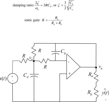
multiple capacitors or inductors into one equivalent capacitor or inductor.) We begin this section with the derivation of the governing differential equation for various second order circuits. At this point we will focus on circuits that we can put into a standard form. Once we have covered Laplace transforms we will analyze different types of second order circuits. This standard second order form will again allow us to easily determine physical characteristics of the circuit and predict the time response. We then solve the differential equations for the case of a constant input.

U

3.1 Governing Differential Equations for Second Order Circuits: Standard FormU

In this section we derive the governing differential equations that model various RL, RC, and RLC