3.0 Second Order Circuits

3.0 Second Order Circuits

A second order circuit is a circuit with two effective energy storage elements, either two capacitors, two inductors, or one of each. (In some circuits it may be possible to combine multiple capacitors or inductors into one equivalent capacitor or inductor ) We begin this section with the derivation of the governing differential equation for various second order circuits. At this point we will focus on circuits that we can put into a standard form. Once we have covered Laplace transforms we will analyze different types of second order circuits. This standard second order form will again allow us to easily determine physical characteristics of the circuit and predict the time response. We then solve the differential equations for the case of a constant input.

3.1 Governing Differential Equations for Second Order Circuits: Standard Form

In this section we derive the governing differential equations that model various RL, RC, and RLC circuits. We then put the governing second order differential equations into a standard form, which allows us to read off descriptive information about the system very easily. The standard form we will use is

2

2 2

( )

( (

(

) )

2 n n ) n

d dy t

dt d

y t

y t K

t x t

ζω ω ω

+ + =

or

2 2

1 ( ) 2

( ) ( ) ( )

n n

d y t d

y t y t

dt dt Kx t

ζ

ω +ω + =

Here we assume the system input isx t( ) and the system output isy t( ). ωn is the system natural frequency, which indicates the frequency at which the system will oscillate if there is no dampling. The natural frequencyω_n has units of radians/second. ζ is the damping ratio, which indicates how much damping there is in the system. A damping ratio of zero indicates there is no damping at all. The damping ratioζ is dimensionaless.

K is the static gain of the system. For a constant input of amplitudeA (x t( )=Au t( ), where u t( ) is the unit step function), in steady state we havedy( )t 0

dt = ,

2 2 ( )t

0 d y

dt = , and . Hence the static gain lets us easily compute the steady state value of the output. To determine the units of the static gain we use

( )=Kx t( )=KA y t

[units of y] = [units of K][units of x] or

[units of K] = [units of y]/[units of x]

derivatives of the inputs. In addition, this form may not always be the best way to write the differential equation.

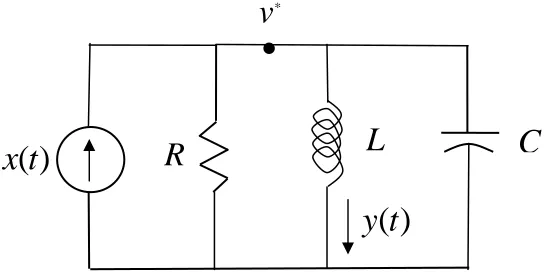
Example 3.2.1. Consider the RLC circuit shown in Figure 3.1.

( )

x t

Figure 3.1. Circuit for Example 3.2.1.

The input, x t( ), is the applied voltage and the output, , is the voltage across the capacitor. If we denote the current flowing in the circuit as , then applying

Kirchhoff’s voltage law around the single loop gives us the equation ( )

y t

( )

i t

( ) ( )

) (

( di t y t i t R

dt

x t L + +

− + ) =0

We can also relate the voltage across the capacitor with the current flowing through the capacitor

( ) ( ) dy t

i t C

dt

=

Substituting this equation into our first expression we get 2

2

( ) ( )

0 ( ) d y t y t( ) RCdy t

dt dt

x t LC + +

− + =

or

2 2

( ) ( )

( ) ( ) d y t dy

LC RC t y

dt + dt + t =x t

Comparing this expression with our standard form we get

natural frequency: 1₂ n

LC

ω = , or

1 n

LC

ω =

damping ratio: 2 n

RC ζ

ω = , or 2

R C L

ζ =

static gain:K =1

( )

y t

+ -

-+

( )

i t

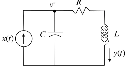
Example 3.2.2. Consider the RLC circuit shown in Figure 3.2.

( )

x t

R

( )

y t

•

*

v

L

C

Figure 3.2. Circuit used in Example 3.2.2.

The input, x t( ), is the applied current and the output, , is the current through the inductor. If we denote the node voltage at the top of the circuit as , then applying Kirchhoff’s current law give us

( )

y t

* ( ) v t

* *

( ) ( )

( ) v t y(t) + Cdv t x t

R dt

= +

We can also relate the voltage across the inductor with the current flowing through the inductor

* ( )

( ) dy t

v t L

dt

=

Substituting this equation into our first expression we get 2

2

( ) ( )

( ) L dy t y(t) + LCd y t x t

R dt dt

= +

or

2 2

( ) ( )

LCd y t L dy t y(t) = x(t) dt +R dt +

Comparing this expression with our standard form we get

natural frequency: 1₂ n

LC

ω = , or

1 n

LC

ω =

damping ratio:2 n

L R ζ

ω = , or

1 2

L C R

ζ =

Example 3.2.3. Consider the RLC circuit shown in Figure 3.3.

R

Figure 3.3. Circuit used in Example 3.2.3.

The input, x t( ), is the applied current and the output, , is the current through the inductor. If we denote the node voltage at the top of the circuit as , then

applyingKirchhoff’s current law give us

( )

y t

* ( ) v t

* ( ) ( ) y(t) + Cdv t x t

dt

=

We can then determine the node voltage v t*( ) as

* ( )

( ) ( ) dy t

v t Ry t L

dt

= +

Substituting this equation into our first expression we get

2 2

( ) ( ) ( )

( ) ( ) d [ ( ) dy t ] ( ) dy t d

x t y t C Ry t L y t RC LC

dt dt dt dt

= + + = + + y t

or

2 2

( ) ( )

( ) ( ) d y t dy t

LC RC y t x t

dt + dt + =

Comparing this expression with our standard form we get

natural frequency: 1₂ n

LC

ω = , or

1 n

LC

ω =

damping ratio:2 n

RC ζ

ω = , or 2

R C L

ζ =

static gain:K =1

C

•

*

v

L

( )

x t

( )

Example 3.2.4. Consider the RLC circuit shown in Figure 3.4.

Figure 3.4. Circuit used in Example 3.2.4.

The input,x t( ), is the applied voltage and the output, y t( ), is the voltage across resistor b

R . Node voltages and are as shown in the figure. Applying Kirchhoff’s current law gives at node gives

( ) a

v t v t_b( ) ( )t a v

( ) ( ) ( ) ( ) ( ) ( ) 0

a a b a a

a

v t x t v t v t v t dv t

C

R R R dt

− −

+ + + =

which we can simplify as

( ) 3 ( ) ( ) ( ) a

a b a

dv t

v t x t v t RC

dt

− − = −

Summing the currents into the negative terminal of the op amp gives us ( ) ( )

0

a b

b

v t dv t

C

R + dt =

or

( )

( ) b

a b

dv t

v t RC

dt

= −

Substituting this expression into our simplified equation above we get

( ) ( )

3 b ( ) ( ) b

b b a b

dv t d dv t

RC x t v t RC RC

dt dt dt

⎡₋ ⎤_{− − = −} ⎡₋ ⎤

⎢ ⎥ ⎢ ⎥

⎣ ⎦ ⎣ ⎦

or

+ -

-+

R

R

R

a

R

b

R

b

C

a

C

( )

x t

( )

y t

+

-

•

•

v

a

2 2

2

( ) ( )

3 ( )

b

a b b

b

b

d t dv t

C C RC v t x t

dt dt

v

R + + =− ( )

Finally, we have

) ( ) ( b

b a b R t y v R R t = + or

( ) a b ( ) b

b

R R

v t y t

R

+ =

resulting in the differential equation 2 2

2

( ) ( )

3 ( )

a b b

a b

b R

d t dy t

C C RC y t x t

dt dt R

y R

R

+ + = −

+ ( )

Comparing this expression with our standard form we get

natural frequency: 2 2 1

a b n

R C C

ω = , or

1 n

a b R C C

ω =

damping ratio:2 3 _b n

RC ζ

ω = , or

3 2 b a C C ζ =

static gain: b

a b R K R R = − +

3.3 Solving Second Order Differential Equations in Standard Form

In this section we will solve second order differential equations the standard form 2 2 2 2 ( ) ( ( ( ) )

2 _{n n} ) _n

d dy t

dt d

y t

y t K

t x t

ζω ω ω

+ + =

for a constant (step) input. We will solve this equation in two parts. We will first determine the natural response, ( . The natural response is the response due only to initial conditions when no inputs are present. Then we will determine the forced

response, . The forced response is the response due to the input only, assuming all initial conditions are zero. The total response is then the sum of the natural and forced responses, ) n y t ( ) f y t

( ) _n( ) _f( )

3.3.1 Natural Response. To determine the natural response we assume there is no input in the system, so we have the equation

2

2 2

( )

) (

(

2 ) 0

n n

n n n

d dy t

dt dt

y t

y t

ζω ω

+ + =

Let’s assume a solution of the form , wherec and are parameters to be determined. Substituting this assumption into the differential equation we get

( ) rt n

y t =c e r

2 2

2 0

rt rt rt

n n

r ec + ζω rce +ω ce =

or

2 2

2 0

[ ]

rt

n n

ce r + ζω r+ω =

Ifc=0 then we are done, and the natural response will bey tn( )=0. This solution certainly satisfies the differential equation. However, ifc≠0, and since can never be zero, we must have

rt

e

2 2

2 _nr _n 0

r + ζω +ω =

Using the quadratic formula, the roots of this equation are

2 2

2 2 2 2

(2 2

) 4

1

2 _{n n n}

n n n n n

r= − ζω ± ζω − ω =−ζω ± ζ ω −ω =−ζω ω ζ± −

We now have four cases to consider depending on the value of the damping ratio ζ . These four cases are: over damped (ζ >1), critically damped (ζ =1), undamped (ζ =0 ), and under damped (0< <ζ 1). We will consider each of these in turn.

Overdamped (ζ >1). In this case we have two real and distinct roots,

2 1

2 2

1 1

n n

n n

r r

ζω ω ζ ζω ω ζ

= − + −

= − − −

The natural response is then

1 2

1 2

( ) r t r t n

y t =c e +c e

where and are constants to be determined by the initial conditions. Note that both and are always negative, since

1

c c2 r1

2

r ζ > ζ2−1.

Critically Damped (ζ =1). In this case we initially appear to have only one solution,

1 2 n

From differential equations, we know that in this situation we should look for an additional solution of the form

( ) rt n

y t =cte

Let’s check to see if this works. With ζ =1, the differential equation becomes 2

2 2

( )

) (

(

2 ) 0

n n

n n n

d dy t

dt dt

y t

y t

ω +ω =

+

We have then

) (

( ) rt rt rt

n d

cte dy t

ce ctre

dt = dt = +

2 2

2 2

2 2

( )

) 2

( rt rt rt rt rt rt rt rt

n

d y t d

ce ctre cre cr d

cte ctr

dt e e cre ctr

dt = =dt⎡⎣ + ⎤ =⎦ + + = + e

] 2 [ ωn]=0 Substituting these into the differential equation we get

2 2 2 2

[2crert +ctr ert] 2+ ωn[cert +ctrert]+ωn[ctrert]=ctert[r +2ωnr+ωn + cert r+

Since we know r= −ω_n this equation is clearly satisfied. Hence our natural solution in this case will be of the form

1 2

( ) rt rt

n e

y t =c +c te

where c1 and c2 are constants to be determined by the initial conditions. Undamped (ζ =0

n

). In this case there is no damping, and the system oscillates at frequency ω . The natural response is of the form

( ) sin( )

n nt

y t =c ω +φ

where cand φ are constants to be determined by the initial conditions.

Under Damped (0< <ζ 1). In this case will have two complex conjugate roots, which we can write as

2 1

n n n d

r= −ζω ± jω −ζ = −ζω ± jω

2 1

d n

ω =ω −ζ is the damped frequency. This is the frequency this system will oscillate with. As we go on, it will be usually easier to remember the roots of this equation as

n d

r= −ζω ± jω = − ±σ jω_d

| |

r

=

ω

2

1

ω

=

ω

−

ζ

Imaginary

+

+

More

Damping

Less

Damping

Real

θ

n

σ ζω

=

Figure 3.5. Relationship between the location of the complex roots(+) and the natural frequency (ω_n, the magnitude of the roots) , the damped frequency (ω_d =ω_n 1−ζ2 , the imaginary part of the root and the frequency of oscillation), and the damping ratio (ζ ,

cos( )θ =ζ ). When ζ =0 (undamped ) the angle and the roots are purely imaginary. In this case

90o

θ =

d n

ω =ω and the system just oscillates at the natural frequency. When ζ =1 (critically damped) the angleθ =0o and the roots are purely real and are repeated. If ζ ≥1 both roots are real, not repeated, and are on the real axis. In this case

0 d

ω = and there is no oscillation. Between these extremes we have an under damped system (0< <ζ 1).

First of all, since our equation for the roots is real we must have complex conjugate roots to the equation, which the figure shows. If we look at the magnitude of the roots, we get

2 * 2 2 2 2 2 2 2 2

( ) ( 1 )

| |r r r n n n n n

2 n

ζω ω ζ ζ ω ω ω ζ

= × = − + − = + − =ω

So the roots will all lie on a circle with magnitude | |r =ω_n. Secondly, if we look at the angle made with the negative real axis, we can see that

cos( ) n n

ζω

θ ζ

ω

When ζ =0 d

(undamped ) the angle and the poles are purely imaginary. In this case

90o

θ =

n

ω =ω and the system just oscillates at the natural frequency. When ζ =1 d

(critically damped) the angleθ =0o and the poles are purely real. In this caseω =0and there is no oscillation. Between these two extremes we have an under damped system (

0< <ζ 1).

Our solution at this point for the natural response to the under damped system is then

( ) ( )

1 2 1 2

( ) n j d t n j d t nt j dt d n

y t =c e−ζω +ω +c e −ζω −ω =e−ζω ⎡_⎣c eω +c e−jωt⎤_⎦

Since we want a real valued solution, let’s make an assumption about the relationship between the two unknown constants. Assume

1

2 2

2 j

j c c e

j c

e c

j

φ

φ

−

=

− =

Then we have

( ) ( )

( ) 2

nt j dt j dt n

c

e e

y t e

j

ζω ω φ ω φ

− _⎡ + ₋ − + _⎤

⎣

= _⎦

Finally we expand this out using Euler’s identity to get

[

]

( ) {co ) sin( )} cos( ) sin(

2 s( { )

nt

n d d d

c

t e t j t t j

j

y = −ζω ω + +φ ω +φ − ω + −φ ω_dt+φ } or

s

( ) nt in( )

n t ce dt

y = −ζω ω +φ

where candφ are constants to be determined by the initial conditions.

3.3.2 Forced Response.

To determine the forced response we must know the system input,x t( ). For now we will assume an input that is zero before t=0 and then has constant amplitude A for t≥0,

0 0

( )

0 t x t

A t

< ≥ ⎧ = ⎨ ⎩

Then for t≥0 we have the equation 2

2 2

( ) ( )

(

2 )

n n

n n n

d dy t

dt dt t A

y t

y K

ω ω

Since this is a linear ordinary differential equation we only need to find one solution. One obvious solution to this equation is the solution in steady state, when

2 2

( ) ( ) 0

f f

d y t dy t

dt = dt = . In steady state we have

( ) f

y t =KA

Note that for a constant input, the steady state output is the product of the static gain and the amplitude of the input.

3.3.3 Total Solution. The total solution to our differential equation is the sum of the natural and forced responses, which is summarized below:

1 2

( ) sin

0 ( )

0 ( 1 ( 1 n , ( ) , ( 1 n n n n t d t t

imaginary roots y t KA c

complex c e roots y t KA ce

rea

undamped t

under damped

l repe d roots y t KA c

real di

t

crititally damped e c te

over damped st roots y

ζω ω ω si ) ) onjugat ate inct

ζ ω φ

ζ ω φ

ζ ζ − − − = + < + = + < = = > + + = + 2 2

( 1) (

1 2

) n n t n n t

t =KA c e+ −ζω ω ζ+ − +c e−ζω ω ζ− −1)

3.4 Response of Under Damped Systems at Rest

For the under damped case, we have the solution sin(

( ) nt )

d

y t =KA+ce−ζω ω t+φ

We will determine the solution assuming the system is initially at rest ( and ). Let’s look first at the derivative term,

(0) 0

y =

(0) 0

y =

( ) sin( ) ( ) cos( )

( ) _nt _nt

n d d d

dy t

t ce

dt ce t

ζω _{ζω ω φ} ζω _{ω ω}

− −

= − + + +φ

At the initial time (t=0) we will have

(0) _nsin( ) _dcos( ) 0 y = −ζω φ ω+ φ = or 2 2 1 1 sin( ) tan( ) cos( ) n d n n

ω ζ ζ

ω

φ _φ

φ ζω ζω

− − = = = = ζ Hence 2 1 1 tan ζ φ ζ − ⎡_⎢ ⎤ ⎣ − ⎢ = ⎥ ⎥⎦

From this we can determine that the hypotenuse of the triangle is r=1, so that 2

) i ( 1

Next we use the initial condition that the initial position is zero, (0) 0 sin( )

y = =KA c+ φ

or

2 sin( ) ₁

KA KA

c

φ _ζ

= − = −

−

Finally, our solution for y t( ) is

2 1

( ) 1 sin( )

1

nt d

y t KA e ζω ω t φ

ζ

−

⎡ ⎤

= ⎢ − + ⎥

−

⎢ ⎥

⎣ ⎦

2 1 1

tan ζ

φ

ζ

− ⎡_⎢ ⎤

⎣ − ⎢

= ⎥

⎥⎦

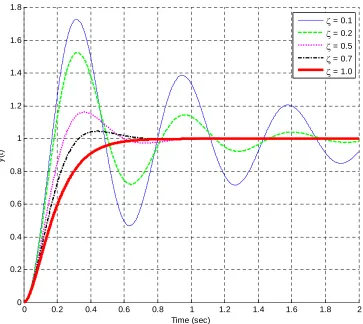
Figure 3.6 shows the response (output) of a system initially at rest. For this systemKA=1 and 10ω_n = rad/sec. There are four responses for under damped systems (0< <ζ 1.0) and one response for a critically damped system (ζ =1.0). The only thing changing in the responses shown in Figure 3.6 is the damping ratio, so it should be clear that the damping ratio can affect the response of the system quite a lot. For example, the peak amplitude and time at which the system reaches the peak amplitude is different for the different responses. Similarly, the frequency at which the system oscillates, the damped frequency, is different for the different responses. Finally, the time it takes the system to reach steady state is different for the different responses.

For systems which fit into our standard second order form, we can predict the response of the system and characterize the response in terms of our parameters (ω ζ_n, ,K). The most common characterizations are depicted in Figure 3.7, which shows the response of a second order system (ω_n =10rad sec/ ,ζ =0.15,K =2.0)initially at rest to a unit step input (an input of constant amplitude 1.0 starting at time zero). Typical characterizations of second order systems shown in the figure are (1) the time to peak ( ), the time it takes the output to reach its peak value; (2) the percent overshoot ( ), which indicates the amount the largest peak of the output overshoots the final (steady state) value of the output; and (3) the settling time (

p

T

PO

s

T ), which indicates the time it takes for the transients in the output to settling out. After the settling time the system output remains within

of the final (steady state) value. (This is a 2% definition of settling time, 1% definitions are also used, though the 1% definition is not as commonly used.) In the following sections we indicate how we can determine these quantities in terms of the parameters that characterize our system.

0 0.2 0.4 0.6 0.8 1 1.2 1.4 1.6 1.8 2 0

0.2 0.4 0.6 0.8 1 1.2 1.4 1.6 1.8

Time (sec)

y(

t)

ζ = 0.1

ζ = 0.2

ζ = 0.5

ζ = 0.7

ζ = 1.0

Figure 3.6. The response (output) of a system initially at rest. For this systemKA=1 and 10

n

ω = rad/sec. There are four responses for under damped systems (0< <ζ 1.0) and one response for a critically damped system (ζ =1.0). The only thing changing in the responses is the damping ratio.

3.4.1 Time to Peak. From our solution to the response of our under damped second order system to a step input, we can determine the time at which reaches its peak value by taking the derivative of and setting it equal to zero. This will give us the maximum value of and the time this occurs at will be called the time to peak, .

( )

y t

( )

y t

( )

y t T_p

[

]

2 ( )

sin( ) cos( ) 0

1 n d d d

dy t KA

t t

dt = − ₋ζ −ζω ω +φ ω+ ω +φ =

sin( ) cos( )

n dt d dt

ζω ω +φ =ω ω +φ

2 2

1 1

tan( ) d n

d

n n

t ω ω ζ ζ

ω φ

ζω ζω ζ

− −

2 1 1 tan dt

ζ

ω φ φ

ζ

− −

+ = =

Hence ω_dt at the time to peak, t=T_p, must equal one period of the tangent, which is π, so

p d

T π

ω

=

Remember thatω_d is equal to the imaginary part of the complex roots of

2 2

2 nr n 0

r + ζω +ω =

Figure 3.7. The response (output) of a system initially at rest. For this systemKA=2, 10

n

ω = rad/sec, and ζ =0.15. Typical characterizations of second order systems (1) the time to peak ( ), the time it takes the output to reach its peak value; (2) the percent overshoot ( ), which indicates the amount the largest peak of the output overshoots the final (steady state) value of the output ; and (3) the settling time (

p

T

PO

s

3.4.2 Percent Overshoot. Evaluating at the peak time we get the maximum value of ,

( )

y t Tp

( )

y t

2 1

) 1 sin(

1

( n pT

p KA e dT

y T ζω ω _p φ)

ζ − ⎡ ⎤ = ⎢ − + ⎥ − ⎢ ⎥ ⎣ ⎦ 2 1

) 1 sin(

1

( n d

p d d KA T e y π ζω ω π ) ω φ ω ζ − ⎡ ⎤ = ⎢ − + ⎥ − ⎢ ⎥ ⎣ ⎦ 2 1 2 1

) 1 sin(

1 ( _p

y T KA e

ζπ ζ ) φ ζ − − ⎡ ⎤ ⎢ ⎥ = + ⎢ − ⎥ ⎣ ⎦

We get the last equation by using the fact thatsin(φ π+ = −) sin( )φ . Finally, since we have previously determined thatsin( )φ = 1−ζ2 ,

2 1 1 ( _p) KA

y T e

ζπ ζ − − ⎡ ⎤ ⎢ ⎥ = + ⎢ ⎥ ⎣ ⎦

The percent overshoot is defined as

) ( ) 10 % ) ( ( 0 p y T Percent Overshoot P

y y O

= = − ∞ ×

∞

Note that this is a standard definition for percent overshoot, independent of the system order or type of system we are analyzing. Note also that the reference level is the value of the function in steady state.

For our under damped second order system we havey( )∞ =KA, so we have

2 1

100%

1 e KA

KA PO KA ζπ ζ − − ⎡ ⎤ ⎢ ⎥ − ⎢ ⎥ ⎣ ⎦ _× + = or 2 1 100% e PO ζπ ζ − − _× =

3.4.3 Settling Time. The settling time of a system is defined as the time it takes for the output of a system with a step input to stay within a given percentage of its final value. We will use the 2% settling time criteria, which is generally four time constants, T_s =4τ. For any exponential decay, the general form is written as t/

constant. Functions of the form e−t/τcos(ω_dt+φ) or e−t/τsin(ω_dt+φ) such as we have in our solution will oscillate, but will still decay at the same rate as the exponential alone. For our system we have 1

n

τ ζω

= or σ ζω= _n, where σ is the absolute value of the real parts of the solutions to . Hence for our system we estimate the settling time as

2 2

2ζωnr ωn 0

+ + = r 4 4 4 s n T τ ζω σ = = =

3.5 Second Order System Examples

Example 3.5.1. Consider the circuit used in Example 3.2.2 with parameter values, ,

10 mH

L= C=10 Fμ , R=40Ω. Assume the input is 0.5 amp step, x t( )=0.5 ( )u t . We can then determine the parameters:

3 6

1 1

)(10 10 )

− −

× × =3,162.2rad / se (10 10

n

LC

ω = = c

3 6 1 10 10

0.395 = 2 (2)(40) 1

1

10 0

L

R C

ζ = = × −₋

× 1 K = 2 2 0.395 0.011se 1 3,162.2 1

p

d _n

T π π π c

ω _{ω ζ}

= = = = − − 4 4 0.032 (0.395)(3162.2) s n T ζω

= = = sec

2 2

0.395

1 _100% 1 0.395 _100%≈_26%

e PO e ζπ π ζ − − − _{× =} − = ×

The time domain expression for the output is then given by

2 2 .395 tan ⎡ ⎤ = ⎢ ⎥= ⎢ ⎥ ⎣ ⎦

1 1 1 1 0 1

tan tan [ ] 1.1647 rad

0.395 ζ φ ζ − ⎡_⎢ ⎤_⎥= − − ⎢ ⎥ ⎣ ⎦ − − ₌ 2.3257 1249.07 2 1

( ) ⎡⎢1 sin(ω +φ)⎤⎥=0.5

⎢ ⎥

⎣ ⎦

[1 1.09 sin(2905.05 1.1647)] 1

nt t

d

y t KA e ζω t t

ζ

−

= − − +

− e

−

Figure 3.8. Response of the circuit used in Example 3.5.1 with parameter values ,

10 mH

L= C=10 Fμ , R=40Ω. Assume the input is 0.5 amp step.

Example 3.5.2. Consider the circuit used in Example 3.2.4 with parameter values, 10

a

C = μF , 1Cb = μF, R=1kΩ,Ra =3kΩ , Rb =2kΩ. Assume the input is a 1 volt step, x t( )=u t( ). We can then determine the parameters:

3 6 6

1 1

316.2 rad / sec 1 10 (10 10 )(1 10 )

n

a b

R C C ω

− −

= = =

× × ×

6 6 3 1 10

0.47

2 2 10 10

3 _b

a C C

ζ = = × −₋ =

×

3

3 3

2 10

0.4 3 10 2 10

b

a b

R K

R R

×

= − = − = −

+ × + ×

2 2 0.011sec

1 316.2 1 0.47 p

d _n

T π π π

ω _{ω ζ}

= = = =

4 4

0.027 sec (0.47)(316.2)

s n

T ζω

= = =

2 2

0.47

1 _100% 1 0.47 _{100% 18.5%}

PO e e

ζπ π

ζ

− −

− _{× =} − _{× ≈}

=

The time domain expression for the output is then given by

2 2

1 1 1 1 0.47 1

tan tan tan [1.657] 1.0815 rad

0.47

ζ φ

ζ

− ⎡ − ⎤₌ − ⎡ − ⎤ −

= ⎢ ⎥=

⎢ ⎥

⎣ ⎦

⎢ ⎥

⎢ ⎥

⎣ ⎦

=

148.6 2

1

( ) 1 sin( ) 0.4[1 1.1329 sin(279.1 1.0815)]

1

nt t

d

y t KA e ζω ω t φ e t

ζ

− −

⎡ ⎤

= ⎢ − + ⎥= − − +

−

⎢ ⎥

⎣ ⎦

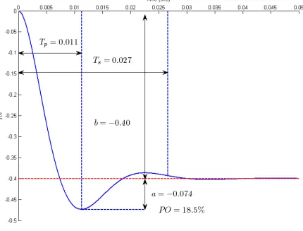
The response for this system is shown in Figure 3.9. Note that although the input is positive, the output has a negative steady state value. This is because the static gain is negative. However, all of the parameters we are interested in (time to peak, settling time, or percent overshoot) are still measured in the same way.

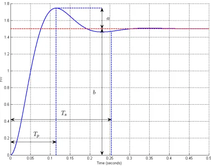
Example 3.5.3. Consider the response of an unknown second order system, with step input 4 volts, x( )t =4 ( )u t

1.5

. The measured output is also in volts. The response of this unknown system is shown in Figure 3.10. We want to try and determine the system parameters from the system output.

For this system, the steady state value is y_ss = ∞ = =y( ) b . Since we know the input was 4, we have KA= y_ss =K(4) 1.5= , or 1.5 0.375

4 4 ss

y

K = = = . The 2% settling time T_s occurs when |y t( )−y_ss|<0.02 for all t≥T_s. Based on this graph, this occurs somewhere near 0.26 seconds, so . The time to peak can be measured off the graph to be approximately 0.11 seconds, so

0.26 sec s

T ≈ T_p

0.11 sec p

T ≈ .To determine the percent overshoot, we first need the steady state value of the output, which we have determined, and then how much beyond this the system has travelled. For this system we have

and . Hence the percent overshoot

is given by

( ) _ss 1.5

y ∞ = y = =b y T( _p)− ∞y( )= ≈a 1.75 1.5− ≈0.25 0.25

100% 100%≈17% 1.5

= ×

a PO

b

Figure 3.9. Response of the circuit used in Example 3.5.2 with parameter values 10

a

Figure 3.10. Output of an unknown second order system, analyzed in Example 3.5.3.

Example 3.5.4. Consider the circuit used in Example 3.2.3 with parameter values, , , . Assume the system is initially at rest and the input is a 1 amp step,

1 mF

C= L=10 mH ( ) ( )

10

R= Ω

x t =u t . We want to determine and characterize the output of the system. We start by determining the system parameters:

3 3

1 1

316.2 rad / sec (10 10 )(1 10 )

n

LC ω

− −

= = =

× ×

3 3 10 1 10

1.581

2 2 10 10

R C L

ζ = = × −₋ =

×

Since ζ >1.0 we have an over damped system. We know from our previous solution we will have a solution of the form

1 2

1 2

( ) r t c r t

e

where

2 2

1 n n 1 (1.581)(316.2) (316.2) 1.581 1 112.7

r = −ζω ω ζ+ − = − + − ≈ −

and

2 2

2

1 (1.581)(316.2) (316.2) 1.581 1 887.1

n n

r = −ζω ω ζ− − = − − − ≈ −

In order to determine the complete response we will use the general form of the solution in what follows. Because the system starts at zero we have the condition

1

(0) 0 ₂

y = =KA+ +c c or c₁+ = −c₂ KA Because the system starts at rest we need to look at the slope

1 2

1 1 2 2 ( ) r t r t

y t =r c e +r c e

At the initial time then we also have

1 1 2 2

(0) 0

y =r c +r c = or 2

1 2

1 c

r c

r

= −

Combining these conditions we have

1 2

1 1

2 2

1 2 2 2 2 2

1

1

r r r r

c c c c c c KA

r r r

⎡ ⎤

=

⎢ ⎥

⎣

−

+ = − + = − = −

⎦

or 2 2

1 1

r

c K

r −r A

= and

2 1

1 2

r KA r

c

r

− =

− . Our solution is then

1 2

2 1

2 1 2 1

( ) 1 r t r t

y t KA r e r e

r −r r −r

⎡ ⎤

= _⎢ − + _⎥

⎣ ⎦

For our system this becomes

112.7 887.1 ( ) 1 1.145 t 0.145 t y t = − e− + e−

The response of this system is displayed in Figure 3.11. As this figure shows, there is no overshoot, so determining the time to peak or percent overshoot is meaningless. We can, however, determine the settling time. However, we cannot use our previous formula

4 s

n

T ζω

= , since this was derived for an under damped system. What we need is to use the more general form that the settling time is equal to four time constants, T_s =4τ. Recall that the general form of a decaying exponential is t/

112.7 / 887.1 /

1

0.00887 sec 112.7

1

, 0.00113 sec 887.1

,

t t

t t

e e

e e

τ

τ

τ

τ

− −

− −

= = =

= = =

The system response and a plot of these exponentials is shown in Figure 3.12. As this figure shows, the response of the exponential with the smaller time constant is much more rapid than the response of the exponential with the larger time constant. The

response of the system is more nearly like the response of the exponential with the larger time constant. Hence, to determine the settling time, we use the largest time constant

4 (4)(0.00887) 0.0355sec s

T = τ ≈ =

This is a general result that we will use later, the response of the system is dominated by the response of the part with the largest time constant.

Figure 3.12. Response of system analyzed in Example 3.5.4 and plots of the exponentials that make up the response. For this system, . This system has components with time constants

112.7 887.1 ( ) 1 1.145 t 0.145 t y t = − e− + e−

1

0.00887 sec 112.7

τ = = and

1

0.00113sec 887.1