ELECTRODIFFUSION MODEL OF RECTANGULAR CURRENT
PULSES IN IONIC CHANNELS OF CELLULAR MEMBRANES∗
CARL L. GARDNER†, JOSEPH W. JEROME‡, AND ROBERT S. EISENBERG§ Abstract. A simplified electrodiffusion model for rectangular current pulses in ionic channels of biological membranes is presented. Numerical simulations and a dynamical systems analysis of traveling wave solutions in the model indicate that the durations and separations of current pulses vary stochastically in time, as is observed experimentally. An electrodiffusion theory of the mechanism for gating is advanced.
Key words. electrodiffusion model, ionic channels, dynamical systems
AMS subject classifications. 76Z99, 92C05
PII.S0036139999351645
1. Introduction. Ionic channels are the main pathway by which the cell communicates—by exchanging substances and electric charge—with its environment. Channels are responsible for signaling in the nervous system, for coordination of mus-cle contraction (including the pumping action of the heart), and for ionic transport in every cell and organ. A substantial fraction of all drugs employed by physicians act directly or indirectly on ionic channels.
Ionic current pulses have been observed experimentally in a wide variety of channels in the membranes of many types of cells (see [1] and references therein). These current pulses are of rectangular wave shape with constant height and are dis-tributed stochastically in time. In this investigation we demonstrate the existence of stochastic-in-time rectangular current pulse traveling waves for a simplified electro-diffusion model of the biological channel developed in analogy with the Gunn diode in semiconductor physics.
We consider a flow of positive ions (cations) in a one-dimensional channel in an electric fieldE(x, t) against a background of negatively charged atoms on the channel protein (“doping” in the semiconductor context). The discrete distribution of charges is described [2, 3, 4] by continuum particle densitiesp(x, t) for the mobile cations and
N for the negatively charged atoms of the protein. We will allowN to be a function of current density and electric field, but not explicitly ofxort. The flow of cations is modeled mathematically by the drift-diffusion (Poisson–Nernst–Planck) model, that is, by a partial differential equation for conservation of the cations and Gauss’s law for the electric field, plus a constitutive law specifying the current densityj(x, t):
∂p ∂t +
1
e ∂j ∂x = 0,
(1)
∗Received by the editors February 5, 1999; accepted for publication (in revised form) April 26,
2000; published electronically September 7, 2000. http://www.siam.org/journals/siap/61-3/35164.html
†Department of Mathematics, Arizona State University, Tempe, AZ 85287-1804 (gardner@
asu.edu). The research of this author was supported in part by the National Science Foundation under grant DMS-9706792 and by DARPA under grant N65236-98-1-5409.
‡Department of Mathematics, Northwestern University, Evanston, IL 60208 ([email protected]).
The research of this author was supported in part by the National Science Foundation under grant DMS-9704458.
§Department of Molecular Biophysics and Physiology, Rush Medical College, Chicago, IL 60612
([email protected]). The research of this author was supported in part by DARPA under grant N65236-98-1-5409.
∂
∂x(E) =e2(p−N),
(2)
j=µpE−eD∂p∂x,
(3)
whereeis the proton charge,is the dielectric coefficient (taken here to be constant),
µis the mobility coefficient, andDis the diffusion coefficient. The usual electric field has been multiplied bye(i.e.,E has units of eV/cm in the cgs system). Typically, in semiconductors bothµandD depend onE.
Periodic and single-pulse (homoclinic) traveling wave solutions [5] for charge den-sity and electric field—and thus for current—are obtained for the Gunn diode when the mobilityµ(E) exhibits negative differential conductance, a region on the current-voltage curve where the current decreases as the voltage is increased. (In fact, dy-namical oscillatory behavior in the Gunn diode occurs for a wide class of models; e.g., the two valley hydrodynamic model produces this behavior [6].) In the biological channel setting, µand D are believed to be very nearly constant for relevant values of E. However, if the charge distributionN on the protein is allowed to depend on current density and electric field—because the protein conformation changes—then rectangular traveling wave current pulses exist in the drift-diffusion model. These traveling waves inpandEpreserve their shape and propagate with constant velocity by balancing drift effects against diffusion.
We will follow Szmolyan’s analysis [5] closely through (6) and (7) below. The drift-diffusion equations for traveling wave solutions are first put into scaled form and integrated once. Then the existence of stochastic-in-time rectangular current pulses for a modelN =N(j, E) with noise will be demonstrated.
2. Drift-diffusion model for traveling waves. To find traveling wave solu-tions, we sets=x−v0tand look for solutionspandE that depend only on s. The
traveling wave velocityv0 is a free parameter and turns out to be on the order of the
ion permeation velocity through the channel. The drift-diffusion equations (1)–(3) become
−ev0dpds = dsd
−µpE+eDdpds
,
(4)
dE ds =
e2
(p−N).
(5)
Equation (4) can be immediately integrated to yield the following scaled equations:
αdpds =pE−E,
(6)
dE ds =
e2
(p−N)≡ e ρ,
(7)
where α =eD/µ and E = ev0/µ. The constant of integration in (6) is set to zero
For traveling wave solutions the current density is simply proportional to the cation density:
j=µ
pE−αdpds
=ev0p.
(8)
The charge density ρ=e(p−N) in Gauss’s law (7) will, in general, depend on the current and the electric field. For the traveling wave solutions we will consider
ρ=ρ(p, E) due to (8).
We know from experimental observations that there is a “rest” value E of the electric field at which the current is constant—either “on” at a valuej+≡ev0p+ or “off” at a valuej−≡ev0p−j+, where the subscripts + and−denote, respectively, the on and off state values. The rest values of the electric field for the on and off states must be the same because of charge conservation: by Gauss’s law,
x+
x−
ρ dx= e(E+−E−) = 0
(9)
only if E+ = E−; E− = 0 since even in the off state there is a nonzero “built in”
potential difference across the cell membrane and thus a nonzero electric field. Here
x+ andx− are locations where the current is, respectively, on or off. The integral of
the charge density from the off to the on state must vanish for the traveling wave, since otherwise an enormous electric field would develop and cause a spark discharge across the cell membrane, destroying the cell, in contradiction to what is observed in nature. Similar remarks apply when integrating from the on to the off state.
The drift-diffusion traveling wave equations mirror this rest-state property since for E = E equation (6) implies p and hence j is constant, and (7) is satisfied if
ρ(p±, E) = 0.
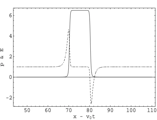
Further, to produce symmetrical rectangular current pulses as solutions to (6) and (7), the charge density in Gauss’s law must be an even function ofE−E. This symmetry property is manifest in Figure 1 (pis a reference ion density defined through (10)) and follows from the invariance of the drift-diffusion traveling wave equations (6) and (7) under the transformationp→p, dp/ds→ −dp/ds,E−E→ −(E−E), and
dE/ds→dE/ds. The reader may check that for a pulse in ion density, the electric field must consist of two equal and opposite spikes because of (6). This symmetry then implies thatρmust be an even function ofE−E.
A simple, physically based model with these properties which produces rectangu-lar current pulses is
ρ(p, E) =−ce(p−p)E
E −1 ,
(10)
where c 1 is a positive constant and p > 0 is a reference ion density at which the slope of E reverses sign. Note that our model has ρ(p, E) = 0 for all p—which produces a line of fixed points for the drift-diffusion traveling wave equations—and is a stronger condition than the constraint above that ρ(p±, E) = 0. See [7] for the characterization of a line of fixed points in terms of the vanishing ofρ(p, E) for allp. The charge density (10) can be derived from a Boltzmann factor. The energy per unit time required to create a current perturbation δj in an electric field E is
50 60 70 80 90 100 110
x - v0t
-2 0 2 4 6
p&E
Fig. 1. Traveling wave solution consisting of a rectangular current pulsep/p∝j (solid line) and electric fieldE/E(dotted line) vs.(x−v0t)E/α.
current perturbation δj =ev0(p−p) is with respect to ev0p. Then the energy per
unit time to turn on a current pulse by creatingδj is
Uon=−v0(p−p)(E−E)ACδxδt, (11)
whereACis the cross-sectional area of the channel andδxandδtare length and time scales over which the current perturbation turns on or off. Note that a factor ofehas been incorporated into our definition of the electric field. To turn off a current pulse by destroyingδj, the energy per unit time is
Uoff=−Uon=v0(p−p)(E−E)ACδxδt. (12)
Since E−E >0 when the current pulse is turned on (see Figure 1) and<0 when the current pulse is turned off, we can writeU as
U =−v0(p−p)|E−E|ACδxδt. (13)
Thus, in our model only the magnitude of displacements ofE fromE matters. We assume that near thermal equilibrium p ≈ p and that N is governed by a Boltzmann factor
N ≈pexp{−U/(kT0)},
(14)
wherekT0is the ambient temperature in energy units. Near thermal equilibrium, the charge density in the channel is
ρ≈ep−epexp{v0(p−p)|E−E|ACδxδt/(kT0)}
≈ −ce(p−p)E
E −1 .
[image:4.612.122.392.83.289.2]Note that the electric field term inρhas the required even symmetry inE−E. With the parameter values chosen below in section 4 to model a K+channel,δxturns out to
be on the order of 0.2 ˚A andδton the order of 10 nanoseconds—which are physically plausible values over which the current perturbation might turn on or off.
We will also add a random noise termσ, representing small charge density fluc-tuations, to the right-hand side of Gauss’s law. We set σ equal to +σ, 0, or −σ, whereσ1 is a positive constant. The nonzero values ofσare randomly distributed with uniform probability in time with zero mean, i.e., with equal probability of being positive or negative. Generating noise±σwith zero mean guarantees charge conser-vation.
We control the frequency of noise by generating a random number r using the C library function random( ) at each timestep and comparingrwith a fixed number
R∈[0,1] which sets the specified frequency. Ifr≥R, then we setσ=±σ, where the sign is chosen randomly. If r < R, we setσ= 0. Thus ifR = 0.999, noise is added on the average once every thousand timesteps.
The magnitude σ should be chosen small enough so as not to visibly affect the height of the current pulses over the course of the simulation (see section 3 below), since these heights are constant to very high accuracy in the experimental data. As long as this condition holds, plots of the computed solutions do not differ visibly with the magnitude of σ. This model for noise generation mimics thermal fluctuations of charge density (where σ corresponds to the average of the absolute value of the thermal fluctuations), since it is theexistenceof small thermal fluctuations of charge density that is important, and not their quantitative magnitude.
The drift-diffusion equations can now be written as
dp dτ =p
E−E,
(16)
dE
dτ =−c(p−p)
EE −1+σ(τ),
(17)
whereτ =s/αandc=αe2c/.
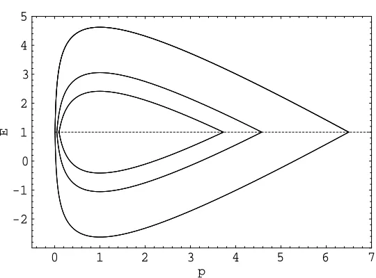
The traveling wave equations (16) and (17) without noise are integrable:
E=E0±c(p−p0−pln(p/p0))/E,
(18)
where the initial conditions are p(τ = 0) =p0 and E(τ = 0) = E0. Equation (18)
may be used to plot phase space orbits.
0 1 2 3 4 5 6 7 p
-2 -1 0 1 2 3 4 5
E
Fig. 2. Heteroclinic orbits in phase space(p/p, E/E)for different initial conditions p0, E0.
The line of fixed points is also shown.
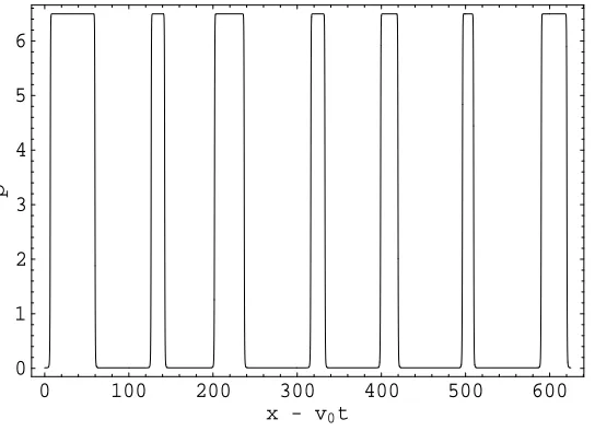
0 50 100 150 200 250 300
x - v0t
0 1 2 3 4 5 6
p
Fig. 3.Solutionp/pvs.(x−v0t)E/αwith random noise added every timestep.
In Figures 3 and 4 we display the solution with noise added every timestep for
p(τ) and total charge density ρ, with p0 = 0.01p, E0 = 1.01E, c = E2/p, and σ=±10−9E2. Recall that the current density j(τ)∝p(τ) and that the integral of
the charge density as the current pulse turns on or off vanishes (preserving charge neutrality). Also note that the physical charge density will be multiplied byc 1, ensuring that the charge density is small in magnitude compared withp.
The solutions are computed from (16) and (17) (and have converged under timestep refinement) using a fourth-order Runge–Kutta method with a fixed timestep ∆t = 0.01 chosen to guarantee that the local truncation error is always less than 10−9. (A
[image:6.612.122.392.88.288.2] [image:6.612.122.397.331.526.2]50 60 70 80 90 100 110
x - v0t
-6 -4 -2 0 2
p-N
Fig. 4.Charge density(p−N)/(cp)∼106(p−N)/pvs.(x−v0t)E/α.
0 100 200 300 400 500 600
x - v0t
0 1 2 3 4 5 6
p
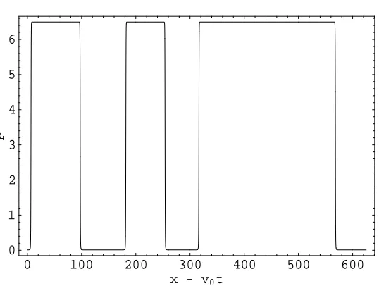
Fig. 5.Solutionp/pvs.(x−v0t)E/αwith random noise added every thousandth timestep on
average.
simulations ensure that the point E =E is not jumped over.) The horizontal axis
x−v0tin the figures may be interpreted at fixedtas space running to the right or at fixedxas time running to the left.
[image:7.612.124.396.324.521.2]0 100 200 300 400 500 600
x - v0t
0 1 2 3 4 5 6
p
Fig. 6.Solutionp/pvs.(x−v0t)E/αwith random noise added every ten thousandth timestep
on average.
0.4
0.42
0.44
0.46
0.48
0.5
0.52
Pulse Duration
0
2000
4000
6000
8000
10000
Number
Fig. 7. Histogram of number of pulses vs. pulse duration in milliseconds for random noise every timestep.
in Figure 7 for a total of approximately 100,000 pulses with noise added every timestep. The exponential decay (above a threshold) of the number of pulses with increasing pulse duration agrees qualitatively with experimental data.
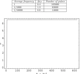
[image:8.612.125.394.85.288.2] [image:8.612.118.391.330.527.2]Table 1
Average pulse duration∆tP in milliseconds and number of pulses for a sample of250seconds
with different average frequencies of adding noise.
Average frequency ∆tP Number of pulses
1 0.4 105000
1/1000 1.3 63000
1/10000 8.8 14000
0 100 200 300 400 500 600
x - v0t
0 1 2 3 4 5 6
p
Fig. 8.Solutionp/pvs.(x−v0t)E/αwithout noise, illustrating that the solution without noise
gets stuck at a fixed point.
timestep the solution cannot get stuck for long at the heteroclinic points. With less frequent noise, the solution may get stuck at a fixed point for a very long time. The elongation of pulse duration with more widely dispersed noise demonstrates conver-gence to the deterministic case (σ = 0) in Figure 8. Note that for the “baseline” solution with noise every timestep the length of an orbit is about 6000 ∆t. We thus expect a phase transition in the behavior of solutions as the frequency of noise falls below once per baseline orbit. It is possible that the two phases may correspond to the two qualitatively distinct forms of gating (“activation” and “inactivation”) experimentally observed in most ionic channels [1].
4. Connection to physical parameter values. We consider here the flow of K+ ions through a channel of diameter 7 ˚A and length 10 ˚A. K+ channels play a
central role in electrical signaling in the nervous system. A typical nerve cell has hundreds of thousands of K+ channels. For the K+ channel, the dielectric constant is on the order of 20, the mobility coefficient µ ≈ 6×10⁻⁵ cm2/(V s), and the
diffusion coefficient D ≈ 1.5×10⁻⁶ cm2/s. Note that the Einstein relation holds: eD/µ=kT0=α, and that in our unitse2= 1.80955×10⁻⁶eV cm.
I and ∆tP in our model are as follows:
I= (6.5p)µEAC, ∆tP = 10αe
µE2, v0=µE/e, c= E2 αe2p.
(19)
The magic numbers 6.5 and 10 in the formulas for I and ∆tP, respectively, come from the simulation results in Figures 3, 5, and 6: pmax ≈ 6.5p for all cases and ∆τP ≈10/Efor the baseline case of noise every timestep.
The simulations presented above thus represent a range of physical values for I, ∆tP,v0,p,N,E, andc. A physically natural magnitude forpwould be a unit charge e spread uniformly throughout the channel volume (2.6×1021 cm−3). We choose p
to be one-half this value so that the average number of ions in the channel when the channel is on is roughly 3.25. We then choose E = 3200 eV/cm in order to make I
equal to 1 picoampere. These values forpandE yield an average pulse duration of 0.4–8.8 milliseconds (see Table 1). The traveling wave velocityv0 = 0.2 cm/s is the
same order of magnitude as the ion permeation velocityvp through the channel. As expected,c= 3.5×10−61.
5. Conclusion. It is remarkable that an electrodiffusion model can produce not only rectangular current pulses, but the wide variety of current behavior observed experimentally in channels of biological membranes. It is difficult to get rectangular waves with flat tops from ordinary differential equations. The addition of noise to the drift-diffusion equations can excite a series of heteroclinic orbits with different current pulse durations and separations but equal heights, in accord with experimental measurements of channel currents. Our model serves as an example where nature may make use of ubiquitous thermal noise to accomplish a biological task—in this case turning the channel on and off.
Physical values predicted in the model, like v0 ∼ vp, ∆tP ∼1–10 milliseconds, E (implies |V|max ∼ 100 millivolts), etc., are of the right order of magnitude for biological channels. A conformational change in the protein and the concomitant small charge fluctuations (c∼10−6) produce gating, rather than a mechanical “flap”
or “slider.” A small dipolar charge wave (a positive spike followed by a negative spike) turns on the current in the channel, and a similar reversed charge wave (a negative spike followed by a positive spike) turns off the current. The relationship of this charge wave to gating current [1] remains to be investigated in the context of a finite channel with realistic boundary conditions.
Our model depends on concentration through the reference ion densityp. How-ever,pis not necessarily coupled to ion densities in the external baths, etc., although it could be. Thus our model can treat both K and Na channels, which are roughly concentration independent, and Ca channels, which are very sensitive to ionic con-centrations.
Alexander [7] investigate the behavior of solutions to a general system of ordinary differential equations with lines of equilibria under various symmetry assumptions. Techniques from these papers may be applicable to a dynamical systems analysis of our current pulse solutions.
We are currently simulating finite channel effects in the full drift-diffusion model. We have recently reproduced the rectangular current pulses in a 10 ˚A long voltage biased channel using the full drift-diffusion model. The finite channel simulations are important because the traveling wave pulses have a length equal to v0∆tP >∼ 1000
channel lengths. This is consistent with experimental measurements of current pulses if the ionic velocities are on the order of vp, since the channel is on for a long time ∆tP compared to an ionic transit time 10 ˚A/vp. Simulating the full drift-diffusion model will allow us to formulate physically relevant boundary conditions for the finite channel. Simulations using the charge model (10) expressed in terms of the currentj
ρ(j, E) =−c v0(j−j)
EE −1,
(20)
wherej =ev0pproduce a nonlinear (sublinear) current-voltage curve, as is observed experimentally (see p. 328 of Hille [1]) and lend credence to the charge model (10). We are also applying our charge model and the current pulse solutions presented here to reproducing “random telegraph noise” current pulses in semiconductor field effect transistors.
REFERENCES
[1] B. Hille,Ionic Channels of Excitable Membranes, Sinauer, Sunderland, MA, 1992.
[2] R. S. Eisenberg, M. M. Klosek, and Z. Schuss,Diffusion as a chemical reaction: Stochastic trajectories between fixed concentrations, J. Chem. Phys., 102 (1995), pp. 1767–1780. [3] W. Nonner, D. Chen, and R. S. Eisenberg,Anomalous mole fraction effect, electrostatics,
and binding, Biophys. J., 74 (1998), pp. 2327–2334.
[4] W. Nonner and R. S. Eisenberg,Ion permeation and glutamate residues linked by Poisson-Nernst-Planck theory in L-type calcium channels, Biophys. J., 75 (1998), pp. 1287–1305. [5] P. Szmolyan,Traveling waves in GaAs-semiconductors, Phys. D, 39 (1989), pp. 393–404. [6] G.-Q. Chen, J. W. Jerome, C.-W. Shu, and D. Wang,Two-carrier semiconductor device
models with geometric structure and symmetry properties, in Modelling and Computa-tion for ApplicaComputa-tions in Mathematics, Science, and Engineering, Oxford University Press, Oxford, UK, 1998, pp. 103–140.
[7] B. Fiedler and S. Liebscher, and J. Alexander, Generic Hopf bifurcation from lines of equilibria without parameters,I. Theory,J. Differential Equations, to appear.
[8] R. P. Feynman, R. B. Leighton, and M. Sands,The Feynman Lectures on Physics, Vol. II, Addison-Wesley, Reading, MA, 1964.
[9] M. Krupa,Robust heteroclinic cycles, J. Nonlinear Sci., 7 (1997), pp. 129–176.