Development and evaluation of an accelerometry system based on inverted pendulum to measure and analyze human balance

Development and evaluation of an accelerometry system

based on inverted pendulum to measure and analyze

human balance

OJIE, Oseikhuemen Davis and SAATCHI, Reza

<http://orcid.org/0000-0002-2266-0187>

Available from Sheffield Hallam University Research Archive (SHURA) at:

http://shura.shu.ac.uk/25064/

This document is the author deposited version. You are advised to consult the

publisher's version if you wish to cite from it.

Published version

OJIE, Oseikhuemen Davis and SAATCHI, Reza (2019). Development and evaluation

of an accelerometry system based on inverted pendulum to measure and analyze

human balance. In: The 32nd International Congress and Exhibition on Condition

Monitoring and Diagnostic Engineering Management, The University of Huddersfield

in West Yorkshire, United Kingdom., 3 Sep 2019 - 5 Sep 2019. (Unpublished)

Copyright and re-use policy

See

http://shura.shu.ac.uk/information.html

Sheffield Hallam University Research Archive

Development and Evaluation of an Accelerometry System Based

On Inverted Pendulum to Measure and Analyze Human Balance

Oseikhuemen Davis Ojie, Reza Saatchi

Sheffield Hallam University, Sheffield, United Kingdom

Email: [email protected]

Abstract. An accelerometry system was developed based on the inverted pendulum model and its effectiveness to measure the body's sway path and sway angle was verified in healthy adult volunteers. Sway path represents the body’s movement from its center of mass position projected to the ground surface while sway angle represents the body's orientation from the vertical. Mathematical models were developed to determine the sway displacement and sway angle from the accelerometry system. The resulting values were compared with the manual measurements obtained from a plumb bob based setup and found to correlate closely. Using the developed system, measures that analyzed the contribution of the visual, somatosensory and vestibular systems to balance were obtained. It was found that the accelerometry system followed the principle of motion of an inverted pendulum and provided information that can assist in better understanding of balance and thus it may assist clinicians in diagnosing balance dysfunctions.

Keywords: Accelerometry, Balance assessment, Sway path, Sway angle.

1

Introduction

Balance disorders have different causes and can be grouped into vertiginous and non-vertiginous disorders [8,9]. Vertiginous disorders (vertigo) are a rotating or spinning motion associated with problems with the vestibular system. Non-vertiginous disorders such as light-headedness, motion intolerance, imbalance, floating, unsteadiness and tilting sensations are associated with cardiovascular diseases, e.g. those found in Parkinson disease [8,9]. Timely diagnosis of balance problems can reduce associated falls [10,11].

Balance examinations can be performed in static and dynamic scenarios using a number of subjective approaches. These approaches have varying complexity, reliability and validity [11]. They include the Berg Balance Scale, the Modified Clinical Test of Sensory Interaction on Balance (M-CTSIB), the Functional Reach Test, the Tinetti Balance Test of the Performance-Oriented Assessment of Mobility Problems, the Timed "Up and Go" Test, and the Physical Performance Test (PPT). Some of these tests are used in balance examination in dynamic conditions (i.e. Berg Scale, Tinetti and Physical Performance Test) while others are suitable for static conditions (i.e. M-CTSIB and Functional Reach Test) [11].

Balance examinations can be based on posturography equipment. Clinically acceptable equipment for posturography should be portable, cost effective, accurate, reliable and easy to use [11]. Force platforms can be used for posturography. They measure the center of foot pressure (COP) displacement in a quiet stance (standing still) position. Force platforms are costly and available only in specialized centers. With the advancement in electronics, miniaturized electronic devices capable of measuring motion have been developed. These devices that are also known as Inertial Measurement Unit (IMUs) are cost effective, can be worn and provide detailed information about the body’s movement. An IMU typically contains an accelerometer that measures directional acceleration (forward/backward) and a gyroscope that indicates the rate of rotation. For the past decades the use of IMUs for measuring human balance has been reported. These provide evidence of the validity of these devices in motion measurements and for balance problem examinations [12,13].

In this paper accelerometry refers to the technique of using an IMU to measure body movement. Accelerometers were used to evaluate static and dynamic balance functions in children [14]. The use of an inertial sensor to quantitatively describe postural control strategy during lying-to-sit-to-stand-to walk tasks has been reported [15]. The majority of these systems only measure dynamic stability. The measurement of standing balance has been reported to play an important role in balance assessment [16]. Standing balance has been evaluated to be useful in the Modified Clinical Test of Sensory Interaction on Balance (M-CTSIB) [16].

2

Accelerometry Technique for Measuring Balance

In the analysis of human balance several authors have provided evidence that body sway during quiet standing can be compared to the motion of an inverted pendulum [17-19]. An inverted pendulum is a pendulum that has its center of mass above its pivot point [19].

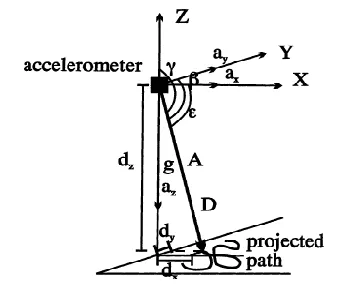
In accelerometry based body sway analysis, the signals from an inertial measurement unit (accelerometer or gyroscope) that is placed on the body's center of mass (COM) position are processed to determine body's movements and orientation angles during a quiet standing position. This sway analysis can provide valuable information such as sway path plot and sway polar plot. A model for evaluating standstill balance is shown in Figure 1 and described by equations 1 and 2, where A is the resultant acceleration, cos α, cos β and cos γ are directional cosines of the accelerations 𝑎𝑥, 𝑎𝑦, and 𝑎𝑧 in the x, y and z axes of the accelerometer, D is the

combined coordinate distance, dz is the position of the sensor from the ground

representing the center of mass position of a body. In this paper centimeters (cm) and centimeters per second square (cm/s2) are used for displacements and accelerations respectively.

Fig. 1. Obtaining the displacement of the tri-axial accelerometer on the ground surface (Source: Mayagoitia et al, (2002)).

𝐴 = √𝑎2𝑥+ 𝑎𝑦2+ 𝑎𝑧 2, cos α =𝑎_𝐴𝑥, cos β =𝑎_𝐴𝑦 𝑎𝑛𝑑 cos γ =𝑎_𝐴𝑧 (1)

𝐷 = − 𝑑𝑧

𝑐𝑜𝑠γ , 𝑑𝑥= 𝐷 cos 𝛼 , 𝑑𝑦= 𝐷 cos 𝛽 (2)

Using this model, the projected displacements from the COM position to the ground, 𝑑𝑥 and 𝑑𝑦, in the x and y directions can be obtained. The equations of the

model are only valid provided the angle swept by the pendulum is small [20]. The limitation of this model relates to not fully conforming to the motion of an inverted pendulum.

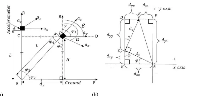
(a) (b)

Fig. 2. Tracing of the sway displacement on the ground: (a) tri-axial accelerometer and (b) gyroscope using an inverted pendulum setup. R is the resultant acceleration in cm/s2. L is the length of the rod in cm. H is the height above the ground surface in cm. 𝑎𝑥, 𝑎𝑦 and 𝑎𝑧 are

accelerations in cm/s2 in the x, y and z axes. α, β , γ, 𝑎 and b are angles in degrees. 𝑑𝑥1 and 𝑑𝑦1

are the resultant displacements in the x and y axes due to the rotational angle 𝜑 in degrees.

𝑑𝑥𝑥, 𝑑𝑥𝑦, 𝑑𝑦𝑦, and 𝑑𝑦𝑥, are coordinate displacements of the x and y axes of 𝑑𝑥, and 𝑑𝑦,

respectively. 𝑑𝑥, and 𝑑𝑦 are ground displacements of the accelerometer.

The resultant acceleration (R) is the same as the resultant acceleration (A) obtained in [20] with directional cosines obtained from equation 1. The following equations can be established for the inclined accelerometer position (labelled as B) as shown in Figure 2(a).

𝜑1= 90 − 𝛾, 𝛾 = 𝛼 − 90, 𝜑1= 180 − 𝛼 (3)

Line CD is parallel to EF (mathematical notation: 𝐶𝐷̅̅̅̅ // 𝐸𝐹̅̅̅̅ ) and Line 𝐶𝐸̅̅̅̅ // 𝐷𝐹̅̅̅̅ thus, 𝜑2= 𝜑1, 𝜑3= 𝛾 (corresponding angles) and 𝜑4= 𝜑2 , 𝜑5= 𝜑3 (alternate

angles). Replacing all angles in Figure 2(a) by their corresponding and alternate angles, the sway displacement in the x axis and the height of the sensor from ground (H) are obtained. Using same operation, the sway displacement in the y axis is computed. These are given as:

𝑑𝑥= −𝐿 cos 𝛼, 𝑑𝑦= −𝐿 cos β , 𝐻 = 𝐿 𝑐𝑜𝑠 𝛾 (4)

In Figure 2(b), the resultant displacements on ground 𝑑𝑥1, and 𝑑𝑦1, from the

gyroscope in the x and y directions can be obtained from equations 5-8, where a and b

are angles defined by the equations. All displacements and angles are in units of cm and degrees respectively. By resolving the angles and displacements, the resultant projected displacements (𝑑𝑥1 and𝑑𝑦1) on ground can be obtained using equations 7

and 8 respectively.

𝑏̂ = 90 − 𝜑̂ , 𝜑̂ = 90 − 𝑏̂ , 𝑎̂ = 90 − 𝑏̂, 𝑎̂=𝜑̂ (5)

𝑑𝑥𝑥 = 𝑑𝑥𝑐𝑜𝑠𝜑 , 𝑑𝑦𝑦= 𝑑𝑦𝑐𝑜𝑠𝜑, 𝑑𝑦𝑥= 𝑑𝑦𝑠𝑖𝑛𝜑, 𝑑𝑥𝑦= 𝑑𝑥𝑠𝑖𝑛𝜑 (6)

𝑑𝑥1 = 𝑑𝑥𝑥− 𝑑𝑦𝑥= 𝑑𝑥𝑐𝑜𝑠𝜑 − 𝑑𝑦𝑠𝑖𝑛𝜑 (7)

𝑑𝑦1= 𝑑𝑦𝑦+ 𝑑𝑥𝑦= 𝑑𝑦𝑐𝑜𝑠𝜑 + 𝑑𝑥𝑠𝑖𝑛𝜑 (8)

3

Evaluation Method of the Mathematical Models

3.1 Accelerometry System Evaluation

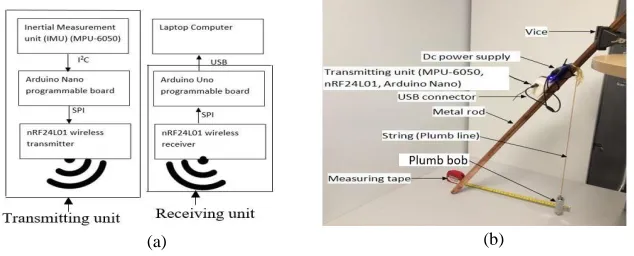
To evaluate the operation of the models an accelerometry system was developed. The system consisted of electronic subunits namely an inertial measurement unit (MPU 6050) with an integrated accelerometer and gyroscope, microcontroller boards (Arduino Nano and Uno board), a wireless transmitter and receiver module. The system has two main sections: the transmitter and receiver as shown in Figure 3(a). The setup used for evaluation consisted of a metal rod, a plumb bob connected to the end of a string which was attached at 100 cm height of the metal rod, and corresponding to the point where the accelerometry transmitting unit was connected as shown in Figure 3(b). The receiving unit of the accelerometry system was connected to a laptop computer using a USB connector. To evaluate the models, the rod was moved to varying angles at steps of 5 degrees from 0 to 45 degrees and its sway measurements (i.e. displacement and angles) were compared with the manual measurements obtained using the plumb bob setup as shown in Figure 3(b). The data of the accelerometer and gyroscope were recorded for 30 seconds at a sampling rate of 60 Hz. Data recording was carried out using Processing© software package and stored in the hard-disk drive of the laptop computer. A measuring tape was used to measure the displacements of the plumb bob on the ground and a protractor was used to measure the orientation angles of the rod. The orientation angle in this study is angle γ in degrees from equation 1.

Fig. 3. Accelerometry system: (a) transmitting and receiving unit (b) andsetup for evaluation

3.2 Balance Evaluation on Human Subjects

Balance evaluation was carried out on 15 healthy volunteers (nine males, six females; mean age and standard deviation: 22.5 and 3.4 years; age range: 18 to 31 years; mean weight and standard deviation: 70.9 and 7.5 kg; weight range: 56.2 to 79.7 kg; mean height and standard deviation: 173.5 and 9.8 cm; height range: 150 to 187.5 cm) with the accelerometry unit placed approximately on the COM position of the subjects. The COM position was just above the hip on the subject's back.

The four conditions defined by the Modified Clinical Test of Sensory Interaction on Balance (M-CTSIB) were used. These are defined as:

 Condition 1: Standing on a firm ground surface with eyes open.

 Condition 2: As in condition 1 but with the eyes closed.

 Condition 3: Standing on a flexible surface (sponge, thickness 8 cm) with eyes open.

 Condition 4: As in condition 3 but with eyes closed.

The data recording lasted for 30 seconds for each test condition. Similar processes of storing the data discussed in section 3.1 were used. Ethical clearance was received from the University prior to recording. The subjects declared to be physically fit and not to have ingested any substance that may affect their balance 48 hours prior to data recording.

3.3 Data Analysis

The data analysis was carried out using MATLAB© and SPSS© packages. The signals from the accelerometer and gyroscope were sampled at 60 Hz and combined using the complimentary filter algorithm shown in equation 9 for better performance to obtain the roll and pitch angle of the IMU device. 𝜃𝑐and 𝜃𝑐−1 represents the current and

previous roll or pitch angle, 𝜃𝑔 is the angular rate of the gyroscope in degrees per

seconds, 𝑑𝑡 is the sample interval (time between successive samples) in second, a is the filter parameter and 𝜑 is the angle obtained from the accelerometer (α or β) in the

x and y axes respectively. The filter parameter (a) was set to 0.8. The obtained angles were inputted into the displacements formulae of equations 2 and 4, to obtain the displacements on ground. The displacements (𝐷_𝑀𝐿𝑛and 𝐷_𝐴𝑃𝑛), velocities (𝑉_𝑀𝐿𝑛and

𝑉_𝐴𝑃𝑛) and accelerations (𝐴_𝑀𝐿𝑛and 𝐴_𝐴𝑃𝑛) on ground in Medio-Lateral (ML) and Anterior-Posterior (AP) directions were obtained using equations 10 and 11, where

𝐷_𝑀𝐿1 and 𝐷_𝐴𝑃1 are the first terms of the displacements in ML and AP directions and the nth and nth-1 terms are current and previous values, and T is the sampling period. The subtraction of the first term of the displacements was used to remove the offsets due to orientation problems of the sensor on the subjects back. Sway measures used to assess balance such as average displacements, velocities and accelerations in the ML and AP directions were computed using equations 12-14. The average displacements (𝐷_{𝑀𝐿𝑎𝑣} and 𝐷_{𝐴𝑃𝑎𝑣}), velocities (𝑉_{𝑀𝐿𝑎𝑣} and 𝑉_{𝐴𝑃𝑎𝑣}) and accelerations (𝐴_{𝑀𝐿𝑎𝑣} and 𝐴_{𝐴𝑃𝑎𝑣}) were measures of the mean of the absolute displacements, velocities and accelerations of the movement of the COM position from the origin, where N is the total number of samples. The range was defined as the difference between the maximum and minimum of each sway measure as shown in equation 15. All displacements, velocities and accelerations were in units of cm, cm/s and cm/s2 respectively.

𝜃𝑐= 𝑎 × (𝜃𝑐−1+ 𝜃𝑔× 𝑑𝑡) + (1 − 𝑎) × 𝜑 (9)

𝐷_𝑀𝐿𝑛= 𝐷_𝑀𝐿𝑛− 𝐷_𝑀𝐿1 , 𝐷_𝐴𝑃𝑛= 𝐷_𝐴𝑃𝑛− 𝐷_𝐴𝑃1, 𝑉_𝑀𝐿𝑛=𝐷𝑀𝐿𝑛−𝐷𝑀𝐿𝑛−1

𝑇 (10)

𝑉_𝐴𝑃𝑛=𝐷𝐴𝑃𝑛−𝐷𝐴𝑃𝑛−1

𝑇 , 𝐴𝑀𝐿𝑛=

𝑉_𝑀𝐿𝑛−𝑉_{𝑀𝐿𝑛−1}

𝑇 , 𝐴𝐴𝑃𝑛=

𝑉_𝐴𝑃𝑛−𝑉_{𝐴𝑃𝑛−1}

𝑇 (11)

𝐷_{𝑀𝐿𝑎𝑣}=_𝑁1

∑

|

|

𝑛=1 , 𝐷_{𝐴𝑃𝑎𝑣} =

1

𝑁

∑

|

|

𝑛=1 (12)

𝑉_{𝑀𝐿𝑎𝑣} =_𝑁1∑𝑁 |𝑉_𝑀𝐿𝑛|

𝑛=1

,

𝐴_{𝑀𝐿𝑎𝑣}=_𝑁1∑𝑁 |𝐴_𝑀𝐿𝑛|

𝑛=1 , 𝐴_{𝐴𝑃𝑎𝑣}=_𝑁1∑𝑁𝑛=1|𝐴_𝐴𝑃𝑛| (14)

𝑅𝑎𝑛𝑔𝑒 = |𝑚𝑎𝑥𝑖𝑚𝑢𝑚 − 𝑚𝑖𝑛𝑖𝑚𝑢𝑚| (15)

The root mean square (rms) values of the displacements (𝐷_{𝑀𝐿𝑅𝑀𝑆} and 𝐷_{𝐴𝑃𝑅𝑀𝑆}), velocities (𝑉_{𝑀𝐿𝑅𝑀𝑆} and 𝑉_{𝐴𝑃𝑅𝑀𝑆}) and accelerations (𝐴_{𝑀𝐿𝑅𝑀𝑆} and 𝐴_{𝐴𝑃𝑅𝑀𝑆}) are the square root of the means of the squared displacements, velocities, and accelerations. The rms values of these measures in ML and AP directions are obtained using equations 16 through 18, where N is the total number of samples.

𝐷_{𝑀𝐿𝑅𝑀𝑆}= √_𝑁1∑𝑁 (𝐷_𝑀𝐿𝑛)2

𝑛=1 , 𝐷_{𝐴𝑃𝑅𝑀𝑆}= √_𝑁1∑𝑁𝑛=1(𝐷_𝐴𝑃𝑛)2 (16)

𝑉_{𝑀𝐿𝑅𝑀𝑆} =

√

𝑁

∑

(𝑉

𝑛=1

,

√

1

𝑁

∑

(

𝑛=1 (17)

𝐴_{𝑀𝐿𝑅𝑀𝑆} =

√

𝑁

∑

𝑛=1 , 𝐴𝐴𝑃𝑅𝑀𝑆=

√

1

𝑁

∑

(

𝑛=1 (18)

4 Results and Discussion

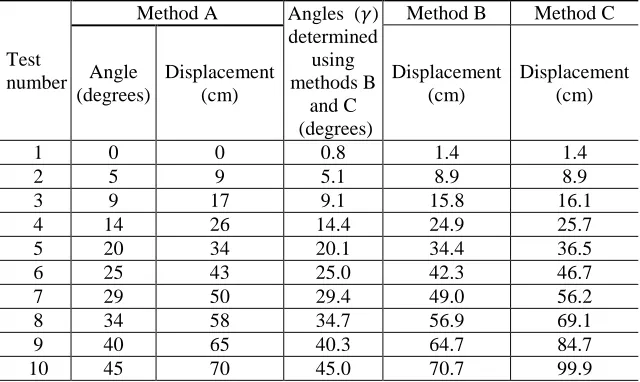
The results of the displacements and angles obtained from the methods are shown in Table 1.

Table 1. Sway measurements obtained using the methods A, B and C. The sway relates to the displacements and angles in the y coordinate axis projected to the ground surface (x=0 cm)

Test number

Method A Angles (𝛾) determined

using methods B

and C (degrees)

Method B Method C

Angle (degrees) Displacement (cm) Displacement (cm) Displacement (cm)

1 0 0 0.8 1.4 1.4

2 5 9 5.1 8.9 8.9

3 9 17 9.1 15.8 16.1

4 14 26 14.4 24.9 25.7

5 20 34 20.1 34.4 36.5

6 25 43 25.0 42.3 46.7

7 29 50 29.4 49.0 56.2

8 34 58 34.7 56.9 69.1

9 40 65 40.3 64.7 84.7

10 45 70 45.0 70.7 99.9

Fig. 4. (a) Displacement differences between the methods and (b) orientation angles

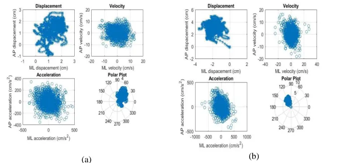
Examples of sway plots produced by the systems for a subject in the conditions 1 and 2 of the M-CTSIB test are shown in Figure 5.

Fig. 5. Examples of displacement, velocity, acceleration and polar plots of a subject from M-CTSIB Test. (a) conditions: 1, (b) condition 2.

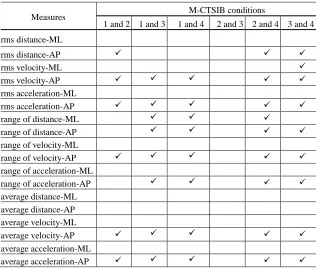
Sway measures used for analyzing conditions 1 to 4 are shown in Table 2. A tick mark indicates significant differences between the sway measures of the compared conditions using both the paired sample t test and the Wilcoxon signed rank test. We observed that there was no difference in the results (i.e. similar results for the tests of significance) of the comparison of the sway measures of the paired sample t test and that of Wilcoxon signed rank test irrespective of whether or not the data conformed to a normal distribution. Five measurement types that provided highest differentiation between the four test conditions were selected from Table 2. The means and standard deviations of their associated measures are provided in Table 3. It was observed that none of the sway measures were able to differentiate between conditions 2 (eyes closed standing on a firm surface) and 3 (eyes open standing on a flexible surface). Among these sway measures, the range, average and rms values of the velocities in the AP direction, and the average and rms values of the accelerations in the AP direction provided higher differentiations amongst the four conditions.

Table 2. Sway measures for the conditions 1 to 4. A tick mark indicates significant differences between the measures of the conditions. Distances, velocities and accelerations are in units of cm, cm/s and cm/s2.

Measures M-CTSIB conditions

1 and 2 1 and 3 1 and 4 2 and 3 2 and 4 3 and 4 rms distance-ML

rms distance-AP   

rms velocity-ML 

rms velocity-AP      rms acceleration-ML

rms acceleration-AP      range of distance-ML   

range of distance-AP     range of velocity-ML

range of velocity-AP      range of acceleration-ML

range of acceleration-AP     average distance-ML

average distance-AP average velocity-ML

average velocity-AP      average acceleration-ML

average acceleration-AP     

Table 3. Means and standard deviations in bracket of the sway measures for the four conditions of M-CTSIB. Velocity in units of cm/s and acceleration in units of cm/s2. 1: Eyes open standing on a firm surface, 2: eyes closed standing on a firm surface, 3: eyes open standing on a flexible surface and 4: eyes closed standing on a flexible surface.

Measures

M-CTSIB conditions

1 2 3 4 rms velocity-AP 2.3 (0.6) 2.7 (0.8) 2.8 (1.0) 3.6 (1.3) rms acceleration-AP 58.6 (15.0) 65.6 (18.8) 69.6(26.9) 85.9 (31.3) range of velocity -AP 16.3 (3.5) 23.5 (12.2) 24.1 (11.0) 33.7 (18.0) average velocity-AP 1.9 (0.5) 2.2 (0.6) 2.2 (0.8) 2.9 (1.0) average acceleration-AP 47.7 (12.8) 53.5 (15.1) 56.8 (21.0) 70.3 (25.2)

5. Conclusion

References

1. Pollock A, Durward B, Rowe P, Paul J (2000) What is balance?. Clinical Rehabilitation 14:402-406. doi: 10.1191/0269215500cr342oa

2. Woollacott M (1993) Age-Related Changes in Posture and Movement. Journal of Gerontology 48:56-60. doi: 10.1093/geronj/48.special_issue.56

3. Shaffer S, Harrison A (2007) Aging of the Somatosensory System: A Translational Perspective. Physical Therapy 87:193-207. doi: 10.2522/ptj.20060083

4. Zalewski C (2015) Aging of the Human Vestibular System. Seminars in Hearing 36:175-196. doi: 10.1055/s-0035-1555120

5. Baker S, Harvey A (1985) Fall Injuries in the Elderly. Clinics in Geriatric Medicine 1:501-512. doi: 10.1016/s0749-0690(18)30920-0

6. Perry B (1982) Falls among the Elderly. Journal of the American Geriatrics Society 30:367-371. doi: 10.1111/j.1532-5415. 1982.tb02833.x

7. Sattin R (1992) Falls Among Older Persons: A Public Health Perspective. Annual Review of Public Health 13:489-508. doi: 10.1146/annurev.publhealth.13.1.489

8. Newman-Toker D, Camargo C (2006) 'Cardiogenic vertigo'—true vertigo as the presenting manifestation of primary cardiac disease. Nature Clinical Practice Neurology 2:167-172. doi: 10.1038/ncpneuro0125

9. Bisdorff A, Staab J, Newman-Toker D (2015) Overview of the International Classification of Vestibular Disorders. Neurologic Clinics 33:541-550. doi: 10.1016/j.ncl.2015.04.010 10. Walker J, Howland J (1991) Falls and Fear of Falling Among Elderly Persons Living in

the Community: Occupational Therapy Interventions. American Journal of Occupational Therapy 45:119-122. doi: 10.5014/ajot.45.2.119

11. Whitney S, Poole J, Cass S (1998) A Review of Balance Instruments for Older Adults. American Journal of Occupational Therapy 52:666-671. doi: 10.5014/ajot.52.8.666 12. Mathie M, Coster A, Lovell N, Celler B (2004) Accelerometry: providing an integrated,

practical method for long-term, ambulatory monitoring of human movement. Physiological Measurement 25: R1-R20. doi: 10.1088/0967-3334/25/2/r01

13. Zheng H, Black N, Harris N (2005) Position-sensing technologies for movement analysis in stroke rehabilitation. Medical & Biological Engineering & Computing 43:413-420. doi: 10.1007/bf02344720

14. Eguchi R, Takada S (2014) Usefulness of the tri-axial accelerometer for assessing balance function in children. Pediatrics International 56:753-758. doi: 10.1111/ped.12370

15. Bagala F, Klenk J, Cappello A et al. (2013) Quantitative Description of the Lie-to-Sit-to-Stand-to-Walk Transfer by a Single Body-Fixed Sensor. IEEE Transactions on Neural Systems and Rehabilitation Engineering 21:624-633. doi: 10.1109/tnsre.2012.2230189 16. Shumway-Cook A, Horak F (1986) Assessing the Influence of Sensory Interaction on

Balance. Physical Therapy 66:1548-1550. doi: 10.1093/ptj/66.10.1548

17. Gatev P, Thomas S, Kepple T, Hallett M (1999) Feedforward ankle strategy of balance during quiet stance in adults. The Journal of Physiology 514:915-928. doi: 10.1111/j.1469-7793.1999. 915ad.x

18. Fitzpatrick R, McCloskey D (1994) Proprioceptive, visual and vestibular thresholds for the perception of sway during standing in humans. The Journal of Physiology 478:173-186. doi: 10.1113/jphysiol. 1994.sp020240

19. Winter D (1995) Human balance and posture control during standing and walking. Gait & Posture 3:193-214. doi: 10.1016/0966-6362(96)82849-9