Using the XCS classifier system for multi objective reinforcement learning problems

Keywords

Action selection, autonomous agents, genetic algorithm, population size

Abstract We investigate the performance of a learning classifier system in some simple multi-objective, multi-step maze problems, using both random and biased action-selection policies for exploration. Results show that the choice of action-selection policy can significantly affect the performance of the system in such environments. Further, this effect is directly related to population size, and we relate this finding to recent theoretical studies of learning classifier systems in single-step problems.

1 Introduction

All living organisms exhibit homeostasis. While the external environment changes constantly, they are able to maintain a relatively constant internal environment; when their ability to do so is compromised, death may swiftly follow. In order to maintain this stability, they must balance many conflicting goals or desires, and dynamically change their actions according to their circumstances. The needs of the moment may override longer-term objectives: the need for food is less than the need to avoid being eaten, the need for shelter may overcome the drive to mate, and so on. Balancing these conflicting drives is the difference between success and failure — between life and death — and the optimization of balancing behaviors is therefore subject to great evolutionary pressure.

For any autonomous artificial entity to perform useful work, it will need to operate in complex problem domains, and also will need to adapt its behavior to optimize the balance of tasks it must perform. In this article we consider the use of an adaptive system — here, a learning classifier system (LCS) [10]— to control an agent that has to solve multi-objective problems. For example, in a simple case, the agent has to seek the shortest path to a goal state while it also needs to maintain its energy levels, in similar fashion to a mobile robot that must perform tasks while maintaining its battery power. The optimal course of action can change dynamically during the course of performing a trial, for its energy levels may be depleted by its actions: the learner is operating in a changing environment.

In particular, we use Wilson’s XCS [18] as detailed in [2]. The ability of XCS to cope with an increased number of objectives and larger maze environments is investigated, paying attention to the choice of action-selection policy.

the population. Results show that the two action-selection schemes can have significant conse-quences for XCS in such domains. In Section 6 we relate these findings to recent theoretical studies of XCS, and in Section 7 we present our conclusions.

2 Related Work

Most complex real-world problems involve multiple objectives that may conflict. There has been a considerable amount of work on multi-objective optimization problems, and numerous researchers have reported success through the application of evolutionary techniques such as genetic algorithms (GAs) [9] — for example, see [6] for an overview.

The first implementation of an LCS, Holland and Reitman’s CS-1 system [11], was a form of multi-objective reinforcement learner, since it included resource reservoirs, which ‘‘reflect simple biological needs’’ and ‘‘deplete regularly in time.’’ Note that the resource reservoirs are not presented to the condition part of the classifiers as the internal environment, but instead influence the choice of which classifier’s action is taken by the learner. A rule’s chance of being chosen is proportional to the specificity of its match to the environment, both internal and external, ‘‘multiplied by the amount of the current needs fulfilled by this classifier’s predicted payoff.’’ The authors outline a simple maze environment where the system starts in the middle and can receive at one end a reward that partially fills the first internal resource reservoir, and at the other end a reward that partially fills the second. The system learns to perform the task and balance its internal needs.

Dorigo and Colombetti [7] used a novel LCS, Alecsys, to control a robot. The main thrust of their work was to evolve simple behaviors, and then combine these to produce more complicated behaviors through a hierarchical system of LCSs. A hierarchy is imposed on a problem, and anLCS coordinatoris introduced to select an action from the LCS lower in the hierarchy. The lower-level LCSs are trained, orshaped, on their task in isolation, and once an acceptable level of performance is obtained for each lower-level module, the rules that it contains are fixed. When this happens, the shaping of the higher coordinating module takes place. Results were obtained for various following/ avoiding tasks in simple environments in which the coordinator switches between different behavioral modules as appropriate; the coordinator switched between behaviors, each attempting to satisfy its own objectives as the global situation required.

Llora and Goldberg [13] present an approach to Pittsburgh-style LCSs [14] — that is, those in which the GA works with complete sets of rules — which is in itself multi-objective, since they con-sider at the same time the following objectives: accuracy of the rules, number of rules, and gener-ality of the solution. In contrast with the work presented in this article, their multiple objectives describe a balancing of desirable characteristics of the learning system by maintaining a Pareto front of nondominated solutions — a balance that is implicit in classifier systems where generality and accuracy are concerned — rather than learning systems solving problems that have multiple objectives.

goals; he examines the latter case. We investigate a similar scenario here.

Gabor et al. [8] have considered similar multi-criteria sequential tasks. Examples of such tasks would include situations where a robot has to perform a number of tasks, but the way in which it per-forms task A can lower the value it will receive from performing task B. The example they give is of ‘‘Buridan’s ass’’: placed between two dishes of food, its hunger drives it to one or the other, but in doing so it raises the possibility that the food on the other dish will be stolen. Since the ass tries to optimize his overall utility, he guards both dishes, thereby eating nothing. He therefore has two different conflicting objectives. We present and examine versions of such sequential multi-objective tasks.

3 XCS: A Brief Description

A population [P] of classifiers is created, each classifier having aconditionand an associated action. Classifier conditions use a ternary encoding with a # (‘‘don’t care’’), allowing generalization. On each discrete time step, amatch set [M] is created, consisting of those rules whose conditions match the current binary input vector from the environment. A system prediction is then formed for each action in [M] according to a fitness-weighted average of the predictions of rules in eachaction set[A], that is, the classifiers in [M] advocating the same action. The system action is then selected either deterministically or randomly (usually with probability 0.5 per trial). If [M] is empty,coveringis used to make a rule whose condition matches the current input, with an equal chance (p#) that each 1 or 0 in

the input vector will be replaced in the new classifier’s condition by a #. Fitness reinforcement in XCS consists of updating three parameters via the Widrow-Hoff delta rule: the predicted payoff (p), the error in that prediction (q), and the fitness (F) for each appropriate rule. The fitness is updated

according to the error relative to those of the other rules within the set. The maximum value of the system’s prediction array is discounted by a factorgand used to update rules from the previous time step. Thus XCS exploits a form of Q-learning [16] in its reinforcement procedure.

The GA acts in [A], that is, niches. Two rules are selected, based on fitness from within the chosen [A]. Rule replacement is global and based on the estimated size of each action set a rule participates in, with the aim of balancing resources across niches. The GA is triggered within a given action set according to the average time since the members of the niche last participated in a GA. The intention is to form a complete and accurate mapping of the problem space through efficient generalizations. In this way, XCS represents a way of using reinforcement learning on complex problems where the number of possible state-action combinations is very large, by discovering efficient generalizations over an underlying Q function. The reader is referred to [2] for a full description of XCS.

We now examine the performance of XCS on a number of simple multi-objective tasks. This takes place in adaptations of the familiar Woods1 grid world [17]. In these and all following experiments, results are the average of 10 experiments, presented as the running average of the last 50 deterministic exploit trials, as in [18].

4 Sequential Multi-objective Maze Problems

with F for ‘‘food.’’ In the experiments described here, three characters are used to encode each state in the environment (to enable future extensions), and the environment is presented to the classifier system as a binary string representing the states of the eight cells that surround the animat’s current position, from north clockwise to northwest. The condition of a classifier has an equal number of characters to the environmental representation. Three characters, allowing the eight possible directions to be represented, again encode the action. The environment is toroidal; every cell has eight neighbors. In the Woods1 environment, the reward given upon reaching the goal is 1,000, and the optimum average path from start to finish is 1.7 steps.

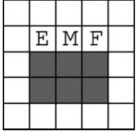
In order to use this, we first present an alteration of the Woods1 environment — Woods1k (Figure 1) — that not only has a food goal, but also has another goal that we call thekey. Each trial starts with the animat not having visited the key state. The reward function gives a payoff of 1,000 in the case that the animat arrives at the goal state when it has visited the key state; the idea being that the key is needed to unlock a door to obtain the reward. In order to allow XCS to know whether the animat has previously visited the key state, an extra character is added to the representation of the environment, this character being set from its initial state of zero to one when the animat visits the key. This can be matched by a concomitant extra character in a classifier’s condition. In Figure 2 the key is shown as K. The optimal average number of steps to the goal state is 3.7. A trial cannot terminate until the key state has been visited before the goal state. 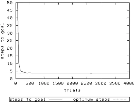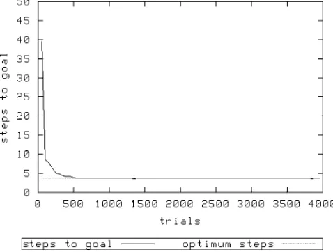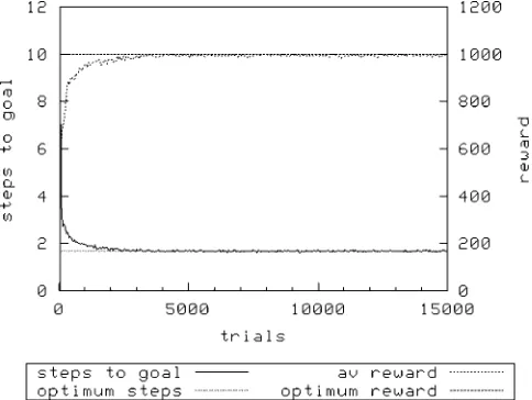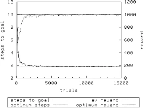Throughout, apart from rule base sizeN, the parameters used areh¼0.2,g¼0.71,u_GA¼25,q0¼0.01,a¼0.1,r¼5,m¼0.8, A¼0.01,udel¼20,y¼0.1,p_#¼0.33, p_I¼10,_qI¼0,F_I¼10,u_sub¼20,u_mna¼8 (see [2]).

Figure 2 shows the performance of XCS with a population sizeNof 1,600 and random exploration. Figure 3 (N¼1,600) and Figure 4 (N¼3,200) show the same treatment using roulette-wheel selection.

Figure 1. Woods1k.

As can be seen, in all treatments XCS achieves optimal performance. However, it would appear that it takes longer to converge to an optimal solution with the roulette action selection mechanism; with

N¼ 1,600 and using random exploration, XCS achieves optimality after about 500 exploit trials, whereas using roulette exploration requires almost double this number of trials with the same value of

N. Increasing Nis required to allow roulette selection to perform as well — here, a doubling ofN. Of course, the above is a rather trivial problem. The animat can only achieve its reward and terminate the trial if it has first visited the key state. A slightly more complicated variant is provided by the same environment, in which the door is always open — Woods1kd. However, the reward gained is dependent on whether the animat has previously visited the key state, being 1,000 if it has, and otherwise 1. Once again, an extra character in both environment and classifier condition allows XCS to know whether the animat has previously visited the key state.

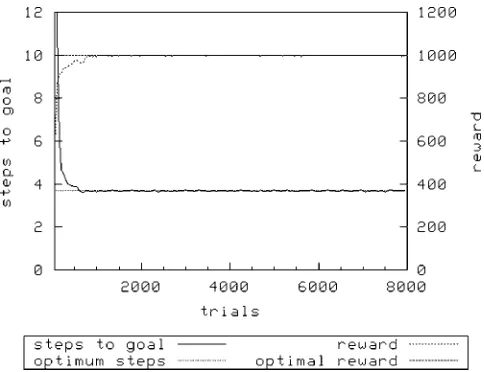
Figure 5 and Figure 6 show the performance of XCS on this second sequential multi-objective task. With both roulette-wheel exploration and random exploration, there is a reduction in the time needed to achieve optimal steps to goal as the population size is increased from 1,600 to 3,200. Once

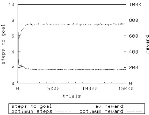
Figure 3. Woods1k,N¼1600, roulette exploration.

again, we also see that random exploration achieves optimal performance faster than with roulette-wheel exploration for the same population size. When N ¼ 1600, the treatment with random exploration clearly achieves a better average reward [1000F0.0 (mean FSD)] than the treatment using roulette-wheel exploration [986F 9.51 (mean F SD)], implying that the map of predicted payoffs is less accurate in the latter. We now examine another class of multi-objective learning problems with XCS, finding a similar pattern emerges.

5 Concurrent Multi-objective Maze Problems

Having seen that XCS is capable of optimal performance on simple, sequential, two-objective problems using both random and roulette-wheel exploration policies, we also considered the more interesting problems where the learner has to juggle multiple simultaneous objectives.

Figure 5. Woods1kd,N¼1600, random exploration.

5.1 Two Objectives

We have used an alteration of the previous Woods1k environment (Figure 7) that not only has a goal state, but also has another goal that we labelenergy(E). In a similar fashion to the sequential multi-objective task, the environment is presented to the classifiers with an additional character, which is set to one if the animat’s internal energy level is higher than 0.5, and otherwise set to zero. The internal energy level varies uniformly, randomly between 0 and 1, and is set at the start of each trial. The classifiers once again have an additional character in the condition that allows them to match this extension of the environment. A trial is terminated and reward is given when the animat reaches either of the goal states.

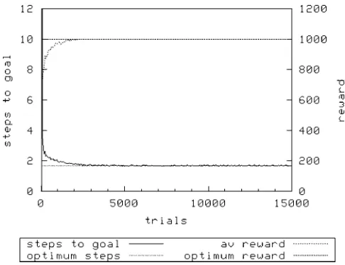
Each trial starts with the animat’s internal energy level initialized uniformly randomly in the range [0, 1]. The reward function is stepwise, giving an external reward of 1,000 in the case that the animat arrives at the energy goal when its energy level is lower than or equal to 0.5, the reward being otherwise 1. Likewise, the animat receives a reward of 1,000 if it arrives at the food goal when its energy level is higher than 0.5, the reward being otherwise 1. The optimal average reward that can be attained is 1,000, and the optimal average number of steps to either goal is 1.7.

Figure 8 shows XCS achieving optimal performance withN¼1,600 using random exploration. In Figure 9 it will be seen that using roulette exploration, performance is slightly worse in terms of the average reward achieved [random 1000F0, roulette 993F3.69 (meanFSD)]. Increasing the population size allows XCS to address this problem using roulette exploration (not shown), again indicating the significance ofNas seen in the sequential problems above.

Figure 7. The Woods1e environment.

Previously, we have presented a version of the Woods1e environment in which the reward received for reaching either goal state is a function of its internal energy level [1]. That is, the re-ward received upon arriving at one or other goal state is directly proportional to the energy level, rather than varying in a stepwise fashion according to the energy level as has hitherto been the case:

at the energy goal; reward ¼ 1000e;

at the food goal; reward ¼ 1000ð1eÞ;

where e is the animat’s internal energy level, which varies between zero and one. As before, this internal energy level is set randomly at the start of each trial, so that half the trials will start withe< 0.5. A cost of 0.01 energy points is deducted for each move made by the animat in the grid world, in the same way that a physical robot’s movement has an energetic cost. The animat’s energy level is not allowed to go below zero. The real value of the internal energy level is hidden from XCS and presented as an extra environmental character set to one if the energy level is above 0.5, otherwise zero. While the optimum number of steps to goal remains 1.7 as in the other parallel multi-objective tasks in the Woods1e environment, the optimum average reward is no longer 1,000, due to the dynamic reward. If the energy level at the goal state is above 0.5, achieving the correct food goal will gain a reward in the range [1000, 500]. The same is true when the animat correctly reaches the energy goal with its energy below 0.5. Assuming an equal random distribution of initial energy levels for trials, the average reward for success is 750. This problem is here called Woods1ef. Since there is a cost of movement, the external reward received by the learner is not only dependent upon initial conditions but also upon its actions.

Figure 10 and Figure 11 show the results using random exploration withN¼1,600 andN¼

3,200, and Figure 12 and Figure 13 show results with roulette-wheel exploration at these values of

N. Using both methods of exploration, XCS was able to solve this problem with a minimum of adjustment, achieving optimal performance simultaneously in terms of both reward achieved and steps taken.

We have so far observed that using roulette-wheel exploration is generally less optimal with smaller populations, compared with random exploration. As can be seen, this is not the case with this problem. Interestingly, withN¼1,600, the treatment using roulette exploration outperforms

the equivalent treatment using random exploration, both in reducing to an optimum the average number of steps taken to the goal state (roulette 1.76F0.03, random 1.98F0.04), and also with respect to the average reward gained (roulette 743 F 7.34, random 714 F 9.97). This result is returned to in Section 6.

5.2 Three Objectives

We have also increased the complexity of the Woods1e task by adding a third goal. The new goal, maintenance, takes priority over the other two goals. We call the resulting task Woods1em (Figure 14). If the animat reaches the maintenance goal and its need for maintenance is higher than or equal to 0.5, it is rewarded 1,000, otherwise 1, irrespective of the internal energy level. If the animat reaches the food goal when the need for maintenance is lower than 0.5 and the energy level is higher than 0.5, it receives a high reward of 1,000, otherwise a low of 1. Likewise, if the animat

reaches the energy goal when the need for maintenance is lower than 0.5 and the energy level is lower than or equal to 0.5, it receives a high reward, otherwise low.

All other experimental details remain as before, except that the condition part of the classifier is extended by a further character, which is set to zero if the animat’s maintenance level is lower than 0.5, and otherwise set to one. As is the case with the internal energy level, the animat’s need for maintenance is set randomly between 0 and 1 at the start of each trial, so that all combinations of high and low maintenance need and high and low energy need are represented in equal numbers of trials. The optimum number of steps to goal increases to around 1.8, and the optimum average reward that can be achieved is once again 1,000. XCS achieves an optimal average reward usingN¼3,200 and random exploration (Figure 15). With an equivalent population size, roulette-wheel exploration takes longer to achieve similar performance, and the system shows more variability in the average reward achieved (Figure 16). Again, doubling the population size allowed XCS with roulette-wheel exploration to achieve results that match those with random exploration (not shown).

5.3 Three Objectives in a Larger Maze

We then further increased the complexity of the task by increasing the size of the environment with a version of the well-known Maze5 [12], which we term Maze5em.

Figure 17 shows Maze5em — a bounded environment containing obstacles (O) and three goal states: food (F), energy (E), and maintenance (M). As before, all environmental states are encoded in three characters, and eight actions are possible. The payoff matrix remains the same as for the three-objective Woods1em problem.

XCS achieves optimality (Figure 18) in the Maze5em environment using random exploration when the probability of having a don’t-care character at each position in the condition isp#¼0.1 and withN¼ 6,400. When p# ¼0.33, some runs are optimal, but some are not, leading to an

average suboptimal performance (not shown). However, it was less easy to achieve similar performance using a roulette-wheel exploration policy. Once again, it was found necessary to increaseNwhen using wheel selection; equivalent performance was achieved with roulette-wheel action selection using the same value ofp#(0.1), and a larger value ofN(8,000).Trials using

p#¼0.33 were never found to perform the task optimally.

This last result is interesting. In all other cases, we have found that roulette-wheel exploration can produce comparable results to that achieved using a random action selection policy at the expense of increasingN. We now see that in this latter, more complex case it is not enough to increaseN; we must also decreasep#. Here p# controls the probability with which alleles in the condition of the rules will have the don’t-care symbol, #. It would appear that XCS is suffering from a greater

tendency to produce overgeneral classifiers in Maze5em. This tendency seems to be exacerbated when using the roulette-wheel action selection policy on explore trials.

We have observed that lowering p#improves XCS’s performance in the three-objective Maze5em problem in the same way it does in Maze5 [12]. Further, roulette-wheel action selection is in effect causing XCS to anneal too fast. That is, the best actions in any particular environmental state are not explored sufficiently, and overgeneral classifiers are allowed to direct the system into suboptimal actions.

6 Roulette-wheel Exploration — Discussion

We now test the hypothesis that increasingNwith roulette action selection improves performance by decreasing the tendency towards excessive generalization. For each experimental treatment of

Figure 17. Maze5em.

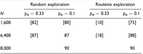
increasing values ofN, withp#¼0.33 orp#¼0.1 and with roulette-wheel action exploration, we examine the average specificity for all classifiers that match in each environmental state for Maze5em. The resulting figures are based on 15,000 exploit trials, and are the average of ten runs (Table 1). With increasing values ofNthere is a tendency for the amount of specificity to increase. Bracketed values indicate that optimal performance wasnotachieved.

The following can be concluded from these results:

_{We have seen that asNincreases, performance is more likely to be optimal.}

_{It is interesting to note that although the two treatments that used random exploration at}

N¼6400 had the same overall specificity (fraction of non-# characters), it was only by using a low value of p#that consistently optimal performance was produced.

_{There is a general tendency for specificity to increase with increasingN.}

_{There is a dramatic difference between the results with roulette selection andp# ¼0.33,}

and those of all other treatments.

It would therefore appear that increasingNreduces the speed at which the roulette-wheel action selection anneals the search within XCS; a larger population size allows more diversity to be maintained for longer, giving the GA more time to weed out the overgeneral rules.

Figure 18. Maze5em, random exploration,N¼6400,p#¼0.1.

Table 1. Percentage of non-general characters in all matching classifiers’ conditions.

Random exploration Roulette exploration

N p#¼0.33 p#¼0.1 p#¼0.33 p#¼0.1

1,600 [82] [80] [10] [75]

6,400 [87] 87 [18] [88]

influence were present, n is the number of actions, and kd is the difficulty of the problem —

determined by the length of the minimum order schema that provides guidance on whether one solution is better than another. This last aspect is illustrated with the extreme case of the parity problem, in which all characters must be specified to correctly predict the outcome; in such a case, any partial solution is as little use as a completely general classifier.

It can be seen from the above equation thatNmust grow with bigger values of both the order of difficultykdand the necessary specificitys[p] in the population. This is based upon the assumption

that binary input strings are encountered that are uniformly distributed over the whole problem instance space {0, 1}l.

As noted above, the Maze5 environment is one in which little generalization is possible, and thus is difficult for XCS. To achieve optimal performance with either action selection mechanism required more specificity (i.e., a lower value ofp#). This is as predicted by the ROP bound above. However,

the assumption that ‘‘binary input strings are encountered . . . uniformly’’ [3] is satisfied neither in multi-step problems (states further from the goal are less frequently visited), nor when the action-selection scheme is other than random. The necessity to further increaseNwhen using roulette-wheel exploration must therefore be due to the effects of bias in sampling frequency on the ROP bound. That is, when using roulette-wheel action selection, higher-payoff action rules will be picked more often than lower-payoff ones. Note that this bias will actually increase as more trials are performed and the payoff values are better approximated by the system. Therefore, new candidate solutions in lower-payoff niches will be much slower to show their accuracy than those in the more frequently visited high-payoff niches. We believe that this explains the necessity to increaseNin order to get equivalent optimality to that achieved with random exploration— the dilution effect reduces the probability of deletion. The differences between individuals are less obvious in a crowd.

Generally then, we have seen that random exploration gives better results for a given value ofN

than roulette-wheel exploration. However, it will be recalled that when we examined the behavior of XCS using random and roulette action selection on the Woods1ef problem with a continuous reward function and associated cost of movement (Section 5.2), we noticed that with lower values ofN, roulette selection outperformed random selection. This contradicts all other results, and requires further explanation.

This problem ( Woods1ef ) in which the seemingly anomalous results occur is a difficult one for XCS to solve, since the reward varies in direct proportion to the animat’s internal energy level when it is at a goal state. There will thus be a high degree of error in all predictions of absolute payoff. Perhaps the results observed in this continuous-reward problem reveal an effect of low values ofN

that have been masked in the other, less challenging problems?

In Figure 19 we see the effect ofNon the performance of XCS in the Woods1ef problem, using the two exploration action-selection strategies. It will be seen that at low values of N, roulette selection strongly outperforms random exploration. A two-tailedt-test demonstrates that there is a statistically significant difference between the treatments in the reward gained at values ofNbetween 600 and 1,400 inclusive. The same is true in the simpler Woods1e problem, as shown in Figure 20. Note that the advantages of roulette action selection are reduced asNrises.

In Figure 19, Figure 20, Figure 21, and Figure 22, ‘‘steps to goal’’ is the average of the last 100 windowed average figures for each run, averaged over ten runs. The ‘‘reward’’ measure is similarly averaged so that it represents the behavior at the end of learning.

areas of the problem space, thus maximizing its overall returns; if resources are scarce, roulette selec-tion can only give this performance advantage if classifiers that predict a lower payoff can be deleted. In XCS there is typically a 90% reduction in fitness from the parents’ values levied on the offspring of classifiers newly produced by the GA. Figure 21 shows how, when this fitness reduction does not occur, roulette-wheel exploration ceases to give such a marked advantage at lower values of

Nfor the Woods1e problem. This supports the hypothesis that roulette-wheel exploration provides a performance advantage by allowing the system to appropriate resources from lower-payoff niches. In less visited niches, offspring would normally have their fitness reduced (as indeed would offspring in all niches). Because the niche is less often visited, they have little chance to boost their fitness by participation in [A] (in the current version of XCS, as used here, and in contrast to Wilson’s original description, fitness increases slowly, since MAM1does not operate on fitness updates, as it is claimed that this ‘‘results in a stronger robustness against inaccurate classifiers’’ [2]). These lower-fitness classifiers then become candidates for deletion when the GA is triggered in a more frequently visited state; the age threshold on deletion is insufficient here. In this way resources are ‘‘stolen’’ from low-payoff state-action niches, since the roulette-wheel exploration strategy increases the bias towards visiting the higher-payoff niches.

Figure 22 shows two areas where XCS experiences the ROP bound. In area 1, at values ofN in-sufficient to satisfy the bound, the roulette-wheel exploration strategy benefits performance through ‘‘resource theft,’’ as described above. Analysis indicates that the suboptimal performance of XCS is not due to thecover challenge[4] — that is, to the population being too small and/or specific to avoid cover firing throughout learning—since for all values ofN,cover occurs infrequently and has stopped after trial 2,000 of a total of 15,000 exploit trials in each experiment (not shown).

In area 2, we suggest that the suboptimal behavior using roulette-wheel exploration is evidence of the effect of the bias on the ROP. As previously stated, the ROP bound is derived on the assumption that all possible states in the space {0, 1}l will be uniformly presented to the system. All other things being equal, this will be true if the exploration policy does not introduce any bias. There is a bias in exploration when using roulette-wheel action selection; higher-payoff classifiers will be picked more often than lower-payoff ones, and this bias will increase as more trials are performed. Therefore, new candidate solutions in lower-payoff niches will be more likely to be deleted before their true accuracy can be

Figure 19. Woods1ef, increasingNwith roulette and random exploration.

determined when using roulette exploration. We believe that this explains the necessity to increaseNin order to get equivalent optimality to that achieved with random exploration—the dilution effect reduces the probability of deletion. The ROP bound is dependent upon the exploration policy.

7 Conclusions

In this article we have shown that XCS can optimally solve a variety of simple multi-objective tasks. It can do so using different action-selection policies in the exploration phase. In the results presented here, we have seen that:

_{XCS can be used successfully with roulette-wheel exploration replacing random action}

selection, suggesting that it may be used for online control where random actions would be inappropriate.

_{Roulette-wheel action selection functions less well than random action selection at}

population sizes sufficient for optimal performance using random action selection. This appears to be due to overgenerality resulting from a lack of exploration.

_{When population sizes are too small for random action selection to perform optimally,}

roulette-wheel action selection may give a performance benefit. This appears to be due to the advantages of concentrating resources on high-payoff niches where there are insufficient resources to form a complete and accurate map of state-action pairs. This may be of value in a robotic environment; smaller populations are less computationally expensive.

_{There is clear evidence for the ROP bound of Butz et al. [3] in multi-step environments,}

but it is critically dependent upon the action-selection policy.

We are now exploiting these findings to use XCS to control a real mobile robot that must solve such multi-objective problems. Investigations of how XCS performs in other types of multi-objective learning tasks are also being undertaken, along with comparisons with other approaches [1].

References

1. Bull, L., & Studley, M. (2002). Consideration of multiple objectives in neural learning classifier systems. InParallel Problem Solving from Nature — PPSN VII(pp. 549 – 557). New York: Springer-Verlag. 2. Butz, M., & Wilson, S. W. (2001). An algorithmic description of XCS. InAdvances in Learning Classifier

Systems: Proceedings of the Fourth International Workshop on Learning Classifier Systems(pp. 253 – 272). New York: Springer-Verlag.

3. Butz, M. V., & Goldberg, D. E. (2003). Bounding the population size in XCS to ensure reproductive opportunities.Evolutionary Computation,11(3), 239 – 278.

4. Butz, M., Kovacs, T., Lanzi, P., & Wilson, S. W. (2004). Toward a theory of generalization and learning in XCS.IEEE Transactions on Evolutionary Computation,8(1), 28 – 46.

5. Crabbe, F. L. (2001). Multiple goal Q-learning: Issues and functions. InProceedings of the International Conference on Computational Intelligence for Modelling Control and Automation (CIMCA). San Mateo, CA: Morgan Kaufmann.

6. Deb, K. (2001).Multi-objective optimization using evolutionary algorithms. New York: Wiley.

7. Dorigo, M., & Colombetti, M. (1998).Robot shaping: An experiment in behavior engineering. Cambridge, MA: MIT Press.

12. Lanzi, P. L. (2000). An analysis of generalization in the XCS classifier system.Evolutionary Computation, 7(2), 125 – 149.

13. Llora, X., & Goldberg, D. E. (2003). Bounding the effect of noise in multiobjective learning classifier systems.Evolutionary Computation,11(3), 278 – 297.

14. Smith, S. F. (1980).A learning system based on genetic adaptive algorithms. Ph.D. thesis. University of Pittsburgh, Pittsburgh, Pennsylvania.

15. Sutton, R. A., & Barto, A. G. (1998).Reinforcement learning: An introduction.Cambridge, MA: MIT Press. 16. Watkins, C. J. C. H. (1989).Learning from delayed rewards. Ph.D. thesis. University of Cambridge,

Cambridge, UK.