Comparing Automatic and Human Evaluation of Local Explanations for
Text Classification
Dong Nguyen♠♦
♠The Alan Turing Institute, London
♦School of Informatics, University of Edinburgh, Edinburgh
Abstract
Text classification models are becoming in-creasingly complex and opaque, however for many applications it is essential that the mod-els are interpretable. Recently, a variety of approaches have been proposed for generat-ing local explanations. While robust evalua-tions are needed to drive further progress, so far it is unclear which evaluation approaches are suitable. This paper is a first step towards more robust evaluations of local explanations. We evaluate a variety of local explanation ap-proaches using automatic measures based on word deletion. Furthermore, we show that an evaluation using a crowdsourcing experi-ment correlates moderately with these auto-matic measures and that a variety of other fac-tors also impact the human judgements.
1 Introduction
While the impact of machine learning is increasing rapidly in society, machine learning systems have also become increasingly complex and opaque. Classification models are usually evaluated based on prediction performance alone (e.g., by measur-ing the accuracy, recall, and precision) and the in-terpretability of these models has generally been undervalued. However, the importance of inter-pretable models is increasingly being recognized (Doshi-Velez and Kim,2017;Freitas,2014).
First, higher interpretability could lead to more effective models by revealing incompleteness in the problem formalization (Doshi-Velez and Kim,
2017), by revealing confounding factors that could lead to biased models, and by supporting error analyses or feature discovery (Aubakirova and Bansal,2016). Second, with the increasing adop-tion of machine learning approaches for humani-ties and social science research, there is also an in-creasing need for systems that support exploratory analyses and theory development.
Various approaches have been explored to in-crease the interpretability of machine learning models (Lipton,2016). This paper focuses on lo-calexplanation, which aims to explain the predic-tion for an individual instance (e.g.,Ribeiro et al.
(2016)). A study byHerlocker et al.(2000) found that providing local explanations could help im-prove the acceptance of movie recommendation systems. Local explanations can come in different forms. For example,Koh and Liang(2017) iden-tify the most influential training documents for a particular prediction. The most common type of local explanation involves identifying the impor-tant parts of the input for a prediction, such as the most predictive words in a document for a text classification model.
In this paper we focus on local explanations for text classification. Below is a fragment of a movie review. The words identified by a local explana-tion method to explain a neural network predicexplana-tion are in bold. The review is labeled with a negative sentiment, but the classifier incorrectly predicted a positive sentiment. The highlighted words help us understand why.
steve martin is one of thefunniestmen alive. if you can take that as a true statement, then your disappointment at this film will equal mine. martin can behilarious,creatingsome of the best laugh-out-loud experiences that have ever taken place in movie theaters. you won’t find any of them here. [...]
Words such as funniestandhilarious were im-portant for the prediction. Besides providing ev-idence for a predicted label, some local expla-nations can also provide evidenceagainst a pre-dicted label. For example, in the above example, the word disappointment was one of the highest ranked words against the predicted label.
Ineffective approaches could generate mislead-ing explanations (Lipton,2016), but evaluating lo-cal explanations is challenging. A variety of ap-proaches has been used, including only visual in-spection (Ding et al.,2017;Li et al.,2016a), intrin-sic evaluation approaches such as measuring the impact of deleting the identified words on the clas-sifier output (Arras et al.,2016), and user studies (Kulesza et al.,2015).
Contributions To further progress in this area, it is imperative to have a better understanding of how to evaluate local explanations. This paper makes the following contributions:
• Comparison of local explanation methods for text classification. We present an in-depth comparison between three local explanation approaches (and a random baseline) using two different automatic evaluation measures on two text classification tasks (Section 4).
• Automatic versus human evaluation. Auto-matic evaluations, such as those based on word deletions, are frequently used since they enable rapid iterations and are easy to repro-duce. However, it is unclear to what extent they correspond with human-based evalua-tions. We show that the automatic measures correlate moderately with human judgements in a task setting and that other factors also impact human judgement. (Section 5).
2 Related Work
Research on interpretable machine learning mod-els has so far mainly focused on computer vision systems (e.g.,Simonyan et al.(2013)). Topic mod-eling is one of the exceptions within NLP where the interpretability of models has been important, since topic models are often valued for their pretability and are integrated in various user inter-faces (Paul,2016). There has recently been an in-creasing interest in improving the interpretability of NLP models, perhaps driven by the increasing complexity of NLP models and the rise of deep learning (Manning,2015).
Globalapproaches aim to provide a global view of the model. One line of work involves mak-ing the machine learnmak-ing model itself more inter-pretable, e.g., by enforcing sparsity or imposing monotonicity constraints (Freitas, 2014). How-ever, often there is a trade-off between accuracy and interpretability as adding constraints to the
model could reduce the performance. An al-ternative involves extracting a more interpretable model, such as a decision tree, from a model that is less interpretable, such as a neural network (Craven,1996). In this case, model performance is not sacrificed but it is essential that the proxy is faithful to the underlying model.
However, often a machine learning model is so complex that interpretable, trustworthy global ex-planations are difficult to attain. Local explana-tions aim to explain the output for an individual instance. For some models the local explanations are relatively easy to construct, e.g., displaying the word probabilities of a Naive Bayes model with respect to each label (Kulesza et al.,2015) or dis-playing the path of a decision tree (Lim et al.,
2009). However, these models may not be easily interpretable if they make use of many features.
For many machine learning models, extracting local explanations is even less straight-forward. Proposed approaches so far include using the gra-dients to visualize neural networks (Aubakirova and Bansal, 2016; Li et al., 2016a; Simonyan et al., 2013), measuring the effect of removing individual words (or features) (Li et al., 2016b;
Martens and Provost, 2014), decomposition ap-proaches (Arras et al., 2016; Ding et al., 2017), and training an interpretable classifier (e.g., lin-ear model) that approximates the neighborhood around a particular instance (Ribeiro et al.,2016). Some approaches have only been evaluated us-ing visual inspection (Ding et al.,2017;Li et al.,
2016a). Goyal et al. (2016) identified impor-tant words for a visual question answering sys-tem and informally evaluated their approach by analyzing the distribution among PoS tags (e.g., assuming that nouns are important). However, quantitative evaluations are needed for more ro-bust comparisons. Such evaluations have included measuring the impact of the deletion of words identified by the explanation approaches on the classification output (Arras et al., 2016, 2017), or testing whether the explanation was consistent with an underlying gold model (Ribeiro et al.,
3 Experimental Setup
This section describes the datasets, the classifica-tion models and the local explanaclassifica-tion approaches used in our experiments.
3.1 Datasets
We experiment with two datasets (Table1):
• Twenty newsgroups (20news). The Twenty
Newsgroups dataset has been used in sev-eral studies on ML interpretability (Arras et al., 2016; Kapoor et al., 2010; Ribeiro et al.,2016). Similar toRibeiro et al.(2016), we only distinguish betweenChristianityand
Atheism. We use the20news-bydate ver-sion, and randomly reserve 20% of the train-ing data for development.
• Movie reviews. Movie reviews with
polar-ity labels (positive versus negative sentiment) fromPang and Lee(2004). We use the ver-sion fromZaidan et al.(2007). The dataset is randomly split into a train (60%), develop-ment (20%) and test (20%) set.
Movie 20news
# training docs 1072 870
# development docs 358 209
# test docs 370 717
label distribution (pos. class) 50.00% 44.49%
Table 1: Dataset statistics
3.2 Text Classification Models
We experiment with two different models. Logis-tic Regression (LR) is implemented using Scikit-learn (Pedregosa et al.,2011) with Ridge regulari-sation, unigrams and a TF-IDF representation, re-sulting in a 0.797 accuracy on the movie dataset and a 0.921 accuracy on the 20news dataset. We experiment with a LR model, because the contri-butions of individual features in a LR model are known. We thus have a ground truth for feature importance to compare against for this model. We also use a feedforward neural network (MLP) im-plemented using Keras (Chollet et al.,2015), with 512 hidden units, ReLU activation, dropout (0.5, not optimized) and Adam optimization, resulting in a 0.832 accuracy on the movie dataset and a 0.939 accuracy on the 20news dataset.
3.3 Local Explanation Methods
In this paper, we focus on local explanation ap-proaches that identify the most influential parts of the input for a particular prediction. In this paper we limit our focus to individual words for explain-ing the output of text classification models. Other representations, e.g., explanations using phrases or higher-level concepts are left for future work. We experiment with explanations for thepredicted
class, since in real-life settings usually no ground truth labels are available. We experiment with the following local explanation approaches:
• Random.A random selection of words in the document.
• LIME (Ribeiro et al., 2016) is a
model-agnostic approach and involves training an interpretable model (in this paper, a linear model with Ridge regularisation) on samples created around the specific data point by per-turbing the data. We experiment with 500– 5000 samples and use the implementation provided by the authors.1
• Word omission. This approach aims to es-timate the contribution of individual words by deleting them and measuring the effect, e.g., by the difference in probability ( Robnik-ˇSikonja and Kononenko,2008). Within NLP, variations have been proposed byK´ad´ar et al.
(2016), Li et al. (2016b) and Martens and Provost(2014). It is also similar to occlusion in the context of image classification, which involves occluding regions of the input image (Zeiler and Fergus, 2014). For LR, this ap-proach corresponds to ranking words accord-ing to the regression weights (and consider-ing the frequency in the text) and is there-fore optimal. For MLP, we use the differ-ence in probability for the predicted class (y) when removing wordˆ w from input x:
p(ˆy|x)−p(ˆy|x\w). This approach supports explanations based on interpretable features (e.g., words) even when the underlying repre-sentation may be less interpretable. However note that in general, this omission approach might not be optimal, since it estimates the contribution of words independently. This approach is also computationally expensive, especially when many features are used.
• First derivative saliency. This approach computes the gradient of the output with re-spect to the input (e.g., used in Aubakirova and Bansal (2016),Li et al.(2016a) and Si-monyan et al. (2013)). The obtained esti-mates are often referred to as saliency values. Several variations exist, e.g.,Li et al.(2016a) take the absolute value. In this paper, the raw value is taken to identify the words important for and against a certain prediction.
4 Automatic Evaluation
In this section we explore automatic evaluation of local explanations. Local explanations should ex-hibit highlocal fidelity, i.e. they should match the underlying model in the neighborhood of the in-stance (Ribeiro et al.,2016). An explanation with low local fidelity could be misleading. Because we generate explanations for the predicted class (rather than the ground truth), explanations with high local fidelity do not necessarily need to match human intuition, for example when the classifier is weak (Samek et al.,2017). Ideally, the evaluation metrics are model agnostic and do not require in-formation that may not always be available such as probability outputs. This paper focuses on local fidelity, but other aspects might also be desired, such as sparsity (Samek et al.,2017;Ribeiro et al.,
2016;Martens and Provost,2014).
4.1 Evaluation Metrics
We measure local fidelity by deleting words in the order of their estimated importance for the predic-tion. Arras et al. (2016) generated explanations with the correct class as target. By deleting the identified words, accuracy increased for incorrect predictions and decreased for correct predictions. However, their approach assumes knowledge of the ground-truth labels.
We take an alternative, but similar, approach. Words are also deleted according to their esti-mated importance, e.g. w1...wnwithw1 the word
with the highest importance score, but for the pre-dicted classinstead. For each document, we mea-sure the number of words that need to be deleted before the prediction switches to another class (the switching point), normalized by the number of words in the document. For example, a value of 0.10 indicates that 10% of the words needed to be deleted before the prediction changed. An ad-vantage of this approach is that ground-truth labels
are not needed and that it can be applied to black-box classifiers, we only need to know the predicted class. Furthermore, the approach acts on the raw input. It requires no knowledge of the underly-ing feature representation (e.g., the actual features might be on the character level). We also experi-ment with the measure proposed bySamek et al.
(2017), referred to as the area over the perturbation curve (AOPC):
AOP C= 1 K+ 1h
K
X
k=1
f(x)−f(x\1..k)ip(x)
wheref(x\1..k)is the probability for the predicted class when words1..kare removed andh·ip(x)
de-notes the average over the documents. This ap-proach is also based on deleting words, but it is more fine-grained since it uses probability values rather than predicted labels. It also enables evalu-ating negative evidence. A drawback is that AOPC requires access to probability estimates of a clas-sifier. In this paper,Kis set to 10.
ForLR, the exact contribution of individual fea-tures to a prediction is known and the words in the document that contributed most to the prediction can be computed directly. For this classifier, the optimal approach corresponds to the omission ap-proach.
4.2 Results
Table 3 reports the results by measuring the ef-fect of word deletions and reporting the aver-age switching point. Lower values indicate that the method was better capable of identifying the words that contributed most towards the predicted class, because on average fewer words needed to be deleted to change a prediction. Table2shows the AOPC values with a cut-off at 10. We measure AOPC in two settings: removing positive evidence (higher values indicate a more effective explana-tion) and negative evidence (lower values indicate a more effective explanation).
Comparison local explanation methods As expected, LIME improves consistently when more samples are used. Furthermore, when comparing the scores of the omission approach for the LR
al-20news (topic) Movie (sentiment)
LR MLP LR MLP
pos. neg. pos. neg. pos. neg. pos. neg.
random 0.0116 0.0101 0.0110 0.0112 0.0073 0.0112 0.0083 0.0066
LIME-500 0.1855 -0.0301 0.1279 -0.0266 0.3168 -0.0786 0.2125 -0.0727
LIME-1000 0.2013 -0.0303 0.1350 -0.0268 0.3509 -0.0793 0.2330 -0.0738
LIME-1500 0.2067 -0.0302 0.1369 -0.0269 0.3586 -0.0794 0.2375 -0.0740
LIME-2000 0.2092 -0.0304 0.1378 -0.0269 0.3628 -0.0794 0.2394 -0.0740
LIME-5000 0.2128 -0.0303 0.1391 -0.0270 0.3693 -0.0794 0.2425 -0.0741
omission 0.2342 -0.0307 0.1422 -0.0272 0.3724 -0.0795 0.2440 -0.0741
[image:5.595.115.489.63.184.2]saliency - - 0.1418 -0.0273 - - 0.2439 -0.0741
Table 2: AOPC results. For each method, AOPC is used to evaluate the words identified to be supportive of the predicted class (positive evidence) and words identified to be supportive of the other class (negative evidence). For LIME, results are reported for different sample sizes.
20news Movie
LR MLP LR MLP
random 0.8617 0.8880 0.6586 0.6843
LIME-500 0.4394 0.5330 0.1747 0.1973
LIME-1000 0.3098 0.4164 0.0811 0.1034
LIME-1500 0.2607 0.3566 0.0613 0.0800
LIME-2000 0.2336 0.3235 0.0547 0.0743
LIME-5000 0.1895 0.2589 0.0474 0.0664
omission 0.1595 0.2662 0.0449 0.0644
[image:5.595.80.284.250.361.2]saliency - 0.2228 - 0.0639
Table 3: The % of words that needs to be deleted to change the prediction (the switching point).
most all cases, the differences are highly signifi-cant (p <0.001), except the difference in average switching point between the omission and salience approach on the movies dataset with theMLP clas-sifier (n.s.) and the difference in average switch-ing point between the omission and LIME-5000 approach on 20news with theMLPclassifier (n.s.). The difference in AOPC scores for evaluating neg-ative evidence was not significant in many cases.
Metric sensitivity First, the results suggest that the values obtained depend strongly on the type of task and classifier. The explanation approaches score better on the sentiment detection task in both Tables 2 and3. For example, fewer words need to be removed on average to change a prediction in the movie dataset (Table 3). A possible explanation is that for sentiment detec-tion, a few words can provide strong cues for the sentiment (e.g., terrific), while for (fine-grained) topic detection (e.g., distinguishing between
Christianityandatheism) the evidence tends to be distributed among more words. Better values are also obtained for theLRclassifier (a linear model) than forMLP.
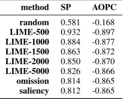
method SP AOPC
random 0.581 -0.168
LIME-500 0.932 -0.897
LIME-1000 0.884 -0.877
LIME-1500 0.863 -0.872
LIME-2000 0.850 -0.870
LIME-5000 0.826 -0.866
omission 0.814 -0.865
saliency 0.812 -0.865
Table 4: Spearman correlation between prediction con-fidence and AOPC and the switching point (SP) for the MLPclassifier on the movie dataset.
Second, as shown in Table2, AOPC enables as-sessing negative evidence (i.e. the words that pro-vide epro-vidence for the opposite class). The obtained absolute values are much smaller compared to the values obtained for the words identified as positive evidence. This is expected, since the positive evi-dence in a document for the predicted class should be larger than the negative evidence.
[image:5.595.354.480.251.352.2]5 Human-based Evaluation
In the previous section we evaluated the local ex-planation approaches using automatic measures. However, the explanations are meant to be pre-sented to humans. We therefore turn to evaluat-ing the explanations usevaluat-ing crowdsourcevaluat-ing. We an-alyze the usefulness of the generated explanations in a task setting and analyze to what extent the au-tomatic measures correspond to the human-based evaluations. The crowdsourcing experiments are run on CrowdFlower. Only crowdworkers from Australia, Canada, Ireland, United Kingdom and the United States and with quality levels two or three were accepted.
5.1 Forward Prediction Task
One way to evaluate an explanation is by ask-ing humans to guess the output of a model based on the explanation and the input. Doshi-Velez and Kim (2017) refer to this as forward simula-tion/prediction. As mentioned byDoshi-Velez and Kim(2017), this is a simplified task. Evaluations using more specific application-oriented tasks or tailored towards specific user groups should be ex-plored in future work. We have chosen the forward prediction task as a first step since it is a general setup that could be used to evaluate explanations for a variety of tasks and models.
In this study, crowdworkers are shown the texts (e.g., a movie review), in which the top words identified by the local explanation approaches are highlighted. Crowdworkers are then asked to guess the output of the system (e.g., a positive or negative sentiment). The crowdworkers are also asked to state their confidence on a five-point Lik-ert scale (‘I am confident in my answer’: strongly disagree . . . strongly agree).
Note that the workers need to guess the out-put of the model regardless of the true label (i.e. the model may be wrong). The crowdworkers are therefore presented with documents with differ-ent prediction outcomes (true positive, true neg-ative, false negneg-ative, and false positive). We sam-ple up to 50 documents for each prediction out-come. A screenshot is shown in Figure1. A quiz and test questions are used to ensure the quality of the crowdworkers. Instructions as well as the test questions included cases where the system made an incorrect prediction, so that workers understood that the task was different than standard labeling tasks. See AppendixAfor more details.
We experiment with the following parameters:
methods (random baseline, LIME with 500 and 5000 samples, word omission, saliency) and the
[image:6.595.308.526.279.422.2]number of words (10, 20). We experiment with both datasets. Due to space constraints, we only experiment with theMLPclassifier. We collected the data in August and September 2017. Each HIT (Human Intelligence Task) was carried out by five crowdworkers. We paid $0.03 per judge-ment. On the 20news dataset, we collected 7,200 judgements from 406 workers (mean nr of. judge-ments per worker: 17.73, std.: 7.21) and on the movie dataset we collected 8,100 judgements from 445 workers (mean nr of. judgements per worker 18.20, std: 7.24).
Figure 1: Screenshot of the task
Confidence Most workers chose confidence val-ues of three or four. Table6reports the confidence scores by method. On the movie dataset, the trends match the intrinsic evaluations closely. The ran-dom method leads to the lowest confidence score, followed by LIME-500 and LIME-5000, and ex-planations from the omission and saliency ap-proach both lead to the highest confidence scores. On the 20news dataset, the trends are less clear. We observe a small, significant negative corre-lation between confidence values and time spent (Spearman correlation:ρ=-0.08,p <0.0001 on the movie dataset,ρ=-0.06,p <0.0001 on 20news).
TP TN FP FN
Method #w Acc Conf n Acc Conf n Acc Conf n Acc Conf n
Movies
random 10 0.652 3.42 250 0.484 3.35 250 0.581 3.26 155 0.355 3.53 155
LIME-500 10 0.848 3.65 250 0.796 3.58 250 0.787 3.41 155 0.710 3.61 155
LIME-5000 10 0.900 3.73 250 0.896 3.70 250 0.852 3.43 155 0.748 3.63 155
omission 10 0.932 3.80 250 0.916 3.67 250 0.845 3.52 155 0.781 3.54 155
saliency 10 0.940 3.87 250 0.872 3.78 250 0.819 3.50 155 0.729 3.59 155
random 20 0.628 3.48 250 0.512 3.43 250 0.471 3.24 155 0.374 3.45 155
LIME-500 20 0.864 3.65 250 0.784 3.51 250 0.742 3.54 155 0.794 3.39 155
LIME-5000 20 0.880 3.76 250 0.864 3.63 250 0.787 3.77 155 0.800 3.67 155
omission 20 0.896 3.95 250 0.884 3.72 250 0.832 3.54 155 0.761 3.58 155
saliency 20 0.860 3.70 250 0.876 3.78 250 0.819 3.63 155 0.806 3.57 155
20news
random 10 0.664 3.45 250 0.656 3.45 250 0.489 3.44 45 0.514 3.47 175
LIME-500 10 0.724 3.53 250 0.768 3.73 250 0.733 3.62 45 0.817 3.84 175
LIME-5000 10 0.740 3.52 250 0.832 3.87 250 0.556 3.29 45 0.697 3.75 175
omission 10 0.652 3.37 250 0.800 3.78 250 0.689 3.31 45 0.754 3.63 175
saliency 10 0.712 3.42 250 0.832 3.77 250 0.689 3.80 45 0.789 3.86 175
random 20 0.616 3.52 250 0.696 3.57 250 0.511 3.84 45 0.537 3.65 175
LIME-500 20 0.668 3.50 250 0.788 3.67 250 0.689 3.22 45 0.697 3.73 175
LIME-5000 20 0.720 3.52 250 0.888 3.86 250 0.667 3.36 45 0.709 3.60 175
omission 20 0.692 3.53 250 0.864 3.80 250 0.644 3.42 45 0.726 3.71 175
[image:7.595.82.517.63.330.2]saliency 20 0.752 3.64 250 0.904 3.74 250 0.711 3.67 45 0.783 3.78 175
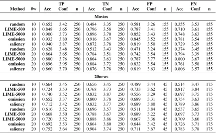
Table 5: Results forward prediction task, with the accuracy (acc), average confidence (conf) and the number of judgements (n). The results are separated according to TP (true positive), TN (true negative), FP (false positive) and FN (false negative) predictions, and the number of words shown (#w).
method accuracy confidence
20news movie 20news movie
random 0.616 0.522 3.520 3.402
LIME-500 0.740 0.798 3.640 3.555
LIME-5000 0.761 0.851 3.665 3.673
omission 0.744 0.868 3.615 3.694
[image:7.595.84.517.66.329.2]saliency 0.790 0.851 3.691 3.701
Table 6: Confidence and accuracy results
Table5separates the results by the different pre-diction outcomes. The results suggest that false positive and false negative are the most revealing. In these cases, crowdworkers are not able to rely on their intuition and a strong explanation should convince them that the system makes a mistake. Otherwise, crowd workers might choose the la-bel matching the document (and not necessarily the classifier output). This is especially salient in the 20news dataset, where the random approach performs better than expected on the true positives and true negatives. For example, compare the ran-dom approach with the omission approach on true positives with ten word explanations.
Our experiments also show that local explana-tions in the form of the most predictive words are sometimes not enough to simulate the output of a system. For example, the best accuracy on true
positive instances in the 20news data is only 0.752. The movie dataset contains difficult instances as well. For example, the omission method identifies the following words in a movie review to explain a false positive prediction: ‘believes’, ‘become’, ‘hair’, ‘unhappy’, ‘quentin’, ‘directed’, ‘runs’, ‘filled’, ‘fiction’, ‘clint’. Due to the composition of the training data, the system has associated words like ‘quentin’ and ‘clint’ with a positive sentiment. This may have confused the crowdworkers as most of them guessed incorrectly. Expanding the ex-planation with for example influential documents (Koh and Liang, 2017) or a visualization of the class distributions of the most influential words could make the explanations more informative.
TP TN FP FN
Noise AOPC Acc Conf n Acc Conf n Acc Conf n Acc Conf n
[image:8.595.83.514.64.145.2]0 0.2627 0.940 3.87 250 0.872 3.78 250 0.819 3.50 155 0.729 3.59 155 0.2 0.2044 0.896 3.60 250 0.780 3.67 250 0.735 3.39 155 0.735 3.58 155 0.4 0.1485 0.824 3.62 250 0.776 3.68 250 0.723 3.37 155 0.645 3.31 155 0.6 0.0851 0.800 3.40 250 0.756 3.40 250 0.710 3.63 155 0.639 3.34 155 0.8 0.0411 0.736 3.29 250 0.640 3.35 250 0.632 3.25 155 0.523 3.25 155
Table 7: Forward prediction task with noisy explanations on the movie dataset and the saliency method
Movie 20news
SP AOPC SP AOPC
tp −0.144** 0.156*** 0.134** −0.161*** fn −0.283*** 0.367***−0.181*** 0.343*** tn −0.195*** 0.153***−0.203***−0.027
[image:8.595.332.502.186.295.2]fp −0.076 0.290***−0.076 0.172
Table 8: Spearman correlation between automatic mea-sures and crowd accuracy. Significance: ∗p < 0.05, ∗∗p <0.01,∗∗∗p <0.001
Dependent variable: crowd accuracy Switching point -0.365∗∗∗(0.023)
Classifier confidence 0.344∗∗∗(0.044)
Prediction outcome: fp 0.053∗∗ (0.021)
Prediction outcome: tn 0.093∗∗∗(0.020)
Prediction outcome: tp 0.132∗∗∗(0.019)
Constant 0.472∗∗∗(0.037)
R2: 0.177 (Adj.: 0.174)
F Stat.: 69.255∗∗∗(df = 5; 1614)
Table 9: OLS results with switching points on the movie data (n = 1,620). ∗p<0.1; ∗∗p<0.05;
∗∗∗p<0.01. Prediction outcome base level = fn.
measured on the true positives in 20news are oppo-site of what we expect. The 20news data is noisy and the classifier picks up on spurious features, possibly confusing the workers.
An example in the 20news data is an e-mail with the following words highlighted: ‘thank’, ‘mail’, ‘discussions’, ‘seminary’, ‘ be-fore’, ‘thanks’, ‘question’, ‘fill’, ‘affected’, ‘ dur-ing’, ‘proofs’. The classifier was confident and the computed switchpoint was low. The e-mail comes from the atheism newsgroup, which becomes clear from reading the text. The highlighted words are all more likely to occur in the christianity news-group, but on their own they are not intuitive to lay people. Consequently, workers guessed incor-rectly that the predicted label was atheism. Expla-nations that also show the negative evidence (in this case, words such as ‘atheism’ and ‘atheists’) and/or the word distributions across classes would likely have led to better crowd accuracy.
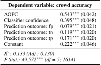
Dependent variable: crowd accuracy
AOPC 0.543∗∗∗(0.042)
Classifier confidence 0.395∗∗∗(0.048)
Prediction outcome: fp 0.079∗∗∗(0.021)
Prediction outcome: tn 0.119∗∗∗(0.020)
Prediction outcome: tp 0.171∗∗∗(0.020)
Constant 0.222∗∗∗(0.046)
R2: 0.133 (Adj.: 0.130)
F Stat.: 49.572∗∗∗(df = 5; 1614)
Table 10: OLS results with AOPC on the movie data (n= 1,620).∗p<0.1;∗∗p<0.05;∗∗∗p<0.01. Prediction
outcome base level = fn.
As shown in section4, the automatic measures correlate strongly with the prediction confidence of the classifier. More words need to be removed before a prediction changes (i.e. a higher switch-ing point) when the classifier is more confident. However, we also find that higher classifier con-fidence leads to higher crowd accuracies (e.g., ρ = 0.236, p < 0.001 on the 20news dataset). We therefore fit an Ordinary Least Squares (OLS) model to control for these different factors (Table
9), with crowd accuracy as the dependent variable. A higher switching point significantly leads to a lower accuracy. However, classifier confidence and prediction outcome also significantly impact the accuracy. Similar trends are observed for the AOPC measure (Table10). We also find that the automatic evaluation measures significantly im-pact crowd accuracy on the 20news dataset, but the patterns are less strong.
6 Conclusion
There has been an increasing interest in improving the interpretability of machine learning systems, but evaluating the quality of explanations has been challenging. This paper focused on evaluating lo-cal explanations for text classification. Lolo-cal ex-planations were generated by identifying impor-tant words in a document for a prediction. We compared automatic evaluation approaches, based on measuring the effect of word deletions, with human-based evaluations. Explanations generated using word omissions and first derivatives both performed well. LIME (Ribeiro et al.,2016) per-formed close to these methods when using enough samples. Our analyses furthermore showed that the evaluation numbers depend on the task/dataset and the confidence of the classifiers.
Next, crowd workers were asked to predict the output of the classifiers based on the generated ex-planations. We found moderate, but significant, correlations between the automatic measures and crowd accuracy. In addition, the human judge-ments were impacted by the confidence of the classifier and the type of prediction outcome (e.g., a false negative versus a true positive). Our re-sults also suggest that only highlighting words is sometimes not enough. An explanation can high-light the most important parts of an input and score well on automatic measures, but if the explanation is not intuitive (for example due to biases in the data), humans are still not able to predict the out-put.
For the classification tasks in this paper (topic classification and sentiment detection) individual words are often predictive. As a result, local expla-nation approaches that select words independently worked well. However, we expect that for tasks where individual words are not predictive, the cur-rent evaluation methods and local explanation ap-proaches may not be sufficient. Furthermore, in future work more fine-grained visualizations (e.g.,
Handler et al.(2016)) could be explored.
Acknowledgements
This work was supported by The Alan Turing Institute under the EPSRC grant EP/N510129/1. The author is supported with an Alan Turing In-stitute Fellowship (TU/A/000006). This work was supported with seed funding award SF023.
References
Leila Arras, Franziska Horn, Gr´egoire Montavon, Klaus-Robert Muller, and Wojciech Samek. 2016. Explaining predictions of non-linear classifiers in NLP. InProceedings of the 1st Workshop on Repre-sentation Learning for NLP. pages 1–7.
Leila Arras, Franziska Horn, Gr´egoire Montavon, Klaus-Robert M¨uller, and Wojciech Samek. 2017. ”What is relevant in a text document?”: An inter-pretable machine learning approach. PLOS ONE
12(8):e0181142.
Malika Aubakirova and Mohit Bansal. 2016. Interpret-ing neural networks to improve politeness compre-hension. In Proceedings of EMNLP 2016. pages 2035–2041.
Chollet et al. 2015. Keras. https://github.
com/fchollet/keras.
Mark W. Craven. 1996. Extracting comprehensible models from trained neural networks. Ph.D. thesis, University of Wisconsin–Madison.
Yanzhuo Ding, Yang Liu, Huanbo Luan, and Maosong Sun. 2017. Visualizing and understanding neural machine translation. In Proceedings of ACL 2017. pages 1150–1159.
Finale Doshi-Velez and Been Kim. 2017. Towards a rigorous science of interpretable machine learning. InarXiv preprint arXiv:1702.08608.
Alex A. Freitas. 2014. Comprehensible classification models: A position paper. SIGKDD Explorations Newsletter15(1):1–10.
Yash Goyal, Akrit Mohapatra, Devi Parikh, and Dhruv Batra. 2016. Towards transparent AI systems: Inter-preting visual question answering models. In Inter-national Conference on Machine Learning (ICML) Workshop on Visualization for Deep Learning.
Abram Handler, Su Lin Blodgett, and Brendan O’Connor. 2016. Visualizing textual models with in-text and word-as-pixel highlighting. In Proceed-ings of the 2016 Workshop on Human Interpretabil-ity in Machine Learning.
Jonathan L. Herlocker, Joseph A. Konstan, and John Riedl. 2000. Explaining collaborative filtering rec-ommendations. InProceedings of CSCW ’00. pages 241–250.
´Akos K´ad´ar, Grzegorz Chrupala, and Afra Alishahi. 2016. Representation of linguistic form and function in recurrent neural networks. CoRR
abs/1602.08952.
Pang Wei Koh and Percy Liang. 2017. Understand-ing black-box predictions via influence functions. In
Proceedings of ICML 2017. pages 1885–1894.
Todd Kulesza, Margaret Burnett, Weng-Keen Wong, and Simone Stumpf. 2015. Principles of explanatory debugging to personalize interactive machine learn-ing. InProceedings of IUI ’15. pages 126–137.
Jiwei Li, Xinlei Chen, Eduard Hovy, and Dan Jurafsky. 2016a. Visualizing and understanding neural mod-els in NLP. InProceedings of NAACL 2016. pages 681–691.
Jiwei Li, Will Monroe, and Dan Jurafsky. 2016b. Un-derstanding neural networks through representation erasure. arXiv preprint arXiv:1612.08220.
Brian Y. Lim, Anind K. Dey, and Daniel Avrahami. 2009. Why and why not explanations improve the intelligibility of context-aware intelligent systems. InProceedings of CHI ’09. pages 2119–2128.
Zachary C. Lipton. 2016. The mythos of model inter-pretability. InProceedings of the 2016 ICML Work-shop on Human Interpretability in Machine Learn-ing (WHI 2016). pages 96–100.
Christopher D. Manning. 2015. Computational lin-guistics and deep learning. Computational Linguis-tics41(4):701–707.
David Martens and Foster Provost. 2014. Explaining data-driven document classifications. MIS Quar-terly38(1):73–100.
Bo Pang and Lillian Lee. 2004. A sentimental educa-tion: Sentiment analysis using subjectivity. In Pro-ceedings of ACL. pages 271–278.
Paul. 2016. Interpretable machine learning: Lessons from topic modeling. In Proceedings of the CHI Workshop on Human-Centered Machine Learning.
Fabian Pedregosa, Ga¨el Varoquaux, Alexandre Gram-fort, Vincent Michel, Bertrand Thirion, Olivier Grisel, Mathieu Blondel, Peter Prettenhofer, Ron Weiss, Vincent Dubourg, Jake Vanderplas, Alexan-dre Passos, David Cournapeau, Matthieu Brucher, Matthieu Perrot, and ´Edouard Duchesnay. 2011. Scikit-learn: Machine learning in Python. Journal of Machine Learning Research12:2825–2830.
Marco Tulio Ribeiro, Sameer Singh, and Carlos Guestrin. 2016. “Why should I trust you?”: Ex-plaining the predictions of any classifier. In Pro-ceedings of KDD ’16. pages 1135–1144.
Marko Robnik-ˇSikonja and Igor Kononenko. 2008. Explaining classifications for individual instances.
IEEE Transactions on Knowledge and Data Engi-neering20(5):589–600.
Wojciech Samek, Alexander Binder, Gregoire Mon-tavon, Sebastian Lapuschkin, and Klaus-Robert M¨uller. 2017. Evaluating the visualization of what
a deep neural network has learned. IEEE Trans-actions on Neural Networks and Learning Systems
28(11):2660 – 2673.
Karen Simonyan, Andrea Vedaldi, and Andrew Zisser-man. 2013. Deep inside convolutional networks: Vi-sualising image classification models and saliency maps. CoRRabs/1312.6034.
Omar Zaidan, Jason Eisner, and Christine Piatko. 2007. Using “annotator rationales” to improve machine learning for text categorization. InProceedings of NAACL 2007. pages 260–267.
Matthew D. Zeiler and Rob Fergus. 2014. Visualiz-ing and understandVisualiz-ing convolutional networks. In
ECCV 2014. pages 818–833.
A Appendix: Crowdsourcing
Test questions were manually selected and were cases for which there should be no doubt about the correct answer (e.g., a simple movie review with only words such as ‘brilliant’, ‘terrific’, etc. high-lighted). Thus, these are questions where work-ers would only fail if they did not pay attention or if they did not understand the task. Explanations were provided for most test questions and were shown after an answer was submitted. The test questions contained instances with different pre-diction outcomes (e.g. false positives and true pos-itives) to make the task clear. To make sure that the test questions did not overlap with the actual HITs (which were generated to explain the predictions of theMLP), the test questions were explanations generated for theLRclassifier.
A quiz with test questions was provided to the crowdworkers when starting the task. If the work-ers performed poorly on the quiz, they were not allowed to continue with the task. Throughout the task, test questions were entered in between the actual HITs (one out of five presented HITs was a test question), to monitor the quality and to flag crowdworkers who performed poorly. We closely monitored the responses to the test questions and in the pilot phase we did remove a few that turned out not be suitable. In the final task, workers per-formed overall very well on the test questions.