Proceedings of the 2nd Clinical Natural Language Processing Workshop, pages 15–21
15
An Analysis of Attention over Clinical Notes for Predictive Tasks
Sarthak Jain Northeastern University [email protected]
Ramin Mohammadi Northeastern university [email protected]
Byron C. Wallace Northeastern University [email protected]
Abstract
The shift to electronic medical records (EMRs) has engendered research into machine learning and natural language technologies to analyze patient records, and to predict from these clinical outcomes of interest. Two ob-servations motivate our aims here. First, un-structured notes contained within EMR often contain key information, and hence should be exploited by models. Second, while strong predictive performance is important, inter-pretability of models is perhaps equally so for applications in this domain. Together, these points suggest that neural models for EMR may benefit from incorporation of at-tentionover notes, which one may hope will both yield performance gains and afford trans-parency in predictions. In this work we per-form experiments to explore this question us-ing two EMR corpora and four different pre-dictive tasks, that: (i) inclusion of attention mechanismsis critical for neural encoder mod-ules that operate over notes fields in order to yield competitive performance, but, (ii) unfor-tunately, while these boost predictive perfor-mance, it is decidedly less clear whether they provide meaningful support for predictions. Code to reproduce all experiments is avail-able athttps://github.com/successar/ AttentionExplanation.
1 Introduction
The adoption of electronic medical records (EMRs) has spurred development of machine learning (ML) and natural language processing (NLP) methods that analyze the data these records contain; for a recent survey of such efforts, see (Shickel et al.,2018). Key information for down-stream predictive tasks (e.g., forecasting whether a patient will need to be readmitted within 30 days) may be contained within unstructured notes fields (Boag et al.,2018;Jin et al.,2018).
In this work we focus on the modules within neural network architectures responsible for en-coding text (notes) into a fixed-size representation for consumption by downstream layers. Patient histories are often long and may contain informa-tion mostly irrelevant to a given target. Encoding this may thus be difficult, and text encoder mod-ules may benefit fromattention mechanisms( Bah-danau et al.,2014), which may be imposed to em-phasize relevant tokens.
In addition to mitigating noise introduced by irrelevant tokens, attention mechanisms are often seen as providing interpretability, or insight into model behavior. However, recent work (Jain and Wallace, 2019) has argued that treating attention as explanation may, at least in some cases, be mis-guided. Interpretability is especially important for clinical tasks, but incorrect or misleading ratio-nales supporting predictions may be particularly harmful in this domain; this motivates our focused study in this space.
To summarize, our contributions are as fol-lows. First, we empirically investigate whether incorporating standard attention mechanisms into RNN-based text encoders improves the perfor-mance of predictive models learned over EMR. We find that they do; inclusion of standard additive attention mechanism in LSTMs consistently yields absolute gains of∼10 points in AUC, compared to an LSTM without attention.1 Second, we evaluate the induced attention distributions with respect to their ability to ‘explain’ model predictions. We find mixed results here, similar to (Jain and Wal-lace, 2019): attention distributions correlate only weakly (though almost always significantly) with
1
gradient measures of feature importance, and we are often able to identify very different attention distributions that nonetheless yield equivalent pre-dictions. Thus, one should not in general treat at-tention weights as meaningful explanation of pre-dictions made using clinical notes.
2 Models
We experiment with multiple standard encoding architectures, including: (i) a standard BiLSTM model; (ii) a convolutional model, and (iii) an embedding projection based model. We cou-ple each of these with an attention layer, follow-ing (Jain and Wallace, 2019). Concretely, each encoder yields hidden state vectors {h1, ..., hT}, and an attention distribution {α1, ..., αT} is in-duced over these according to a scoring function
φ: αˆ = softmax(φ(h)) ∈ RT. In this work we considerAdditivesimilarity functionsφ(h) =
vTtanh(W1h+b)(Bahdanau et al.,2014), where
v,W1,b are model parameters. Predictions are made on the basis of induced representations:yˆ=
σ(θ·hα)∈R|Y|, wherehα =PTt=1αˆt·htandθ are top-level discriminative (e.g., softmax) param-eters.
3 Datasets and Tasks
We consider five tasks over two independent EMR datasets. The first EMR corpus is MIMIC-III (Johnson et al.,2016), a publicly available set of records from patients in the Intensive Care Unit (ICU). We follow prior work in modeling aims and setup on this dataset. Specifically we consider the following predictive tasks on MIMIC.
1. Readmission. The task here is to predict pa-tient readmission within 30 days of discharge or transfer from the ICU. We follow the cohort selection of (Lin et al.,2018). We assume the model has access to all notes from patient ad-mission up until the discharge or transfer from the ICU (the point of prediction).
2. Retrospective 1-yr mortality. We aim to pre-dict patient mortality within one year. In this we follow the experimental setup of (Ghassemi et al.,2014). The model is provided all notes up until patient discharge (excluding the discharge summary).
3. Phenotyping. Here we aim to predict the top 25 acute care phenotypes for patients (asso-ciated at discharge with the admission). For
this we again rely on the framing established in prior work (Harutyunyan et al.,2017). The model has access to all notes from admission up until the end of the ICU stay. Note that this may be viewed as a multilabel classifica-tion task, similar to (Harutyunyan et al.,2017;
Lipton et al.,2015).
The second EMR dataset we use comprises records for 7174 patients from Mass General Hos-pital who underwent hip or knee arthroplasty pro-cedures. Use of this data was approved by an In-stitutional Review Board (IRB protocol number 2016P002062) at Partners Healthcare.
1. Predicting Hip and Knee Surgery Compli-cations. We consider patients who underwent hip or knee arthroplasty procedure; we aim to classify these patients with respect to whether or not they will be readmitted within 30 days due to surgery-related complications. We run experiments over hip and knee surgery patients separately.
4 Experiments
Following the analysis of (Jain and Wallace,2019) but focusing on clinical tasks, we perform a set of experiments on these corpora that aim to assess the degree to which attention mechanisms aid (or hamper) predictive performance, and the degree to which the induced attention weights might be viewed as providing explanations for predictions.
0.0 0.5 1.0 Median Output Difference [0.00, 0.25) [0.25, 0.50) [0.50, 0.75) [0.75, 1.00) Max attention (a) Readmission
0.0 0.5 1.0
[0.00, 0.25) [0.25, 0.50) [0.50, 0.75) [0.75, 1.00) (b) Mortality
0.0 0.5 1.0
[0.00, 0.25) [0.25, 0.50) [0.50, 0.75) [0.75, 1.00)
(c) Knee Surgery
0.0 0.5 1.0
[0.00, 0.25) [0.25, 0.50) [0.50, 0.75) [0.75, 1.00)
(d) Hip Surgery
0.0 0.5 1.0
[0.00, 0.25) [0.25, 0.50) [0.50, 0.75) [0.75, 1.00) (e) Phenotyping
0.0 0.5 1.0
Median Output Difference [0.00, 0.25) [0.25, 0.50) [0.50, 0.75) [0.75, 1.00) Max attention (f) Readmission
0.0 0.5 1.0
[0.00, 0.25) [0.25, 0.50) [0.50, 0.75) [0.75, 1.00) (g) Mortality
0.0 0.5 1.0
[0.00, 0.25) [0.25, 0.50) [0.50, 0.75) [0.75, 1.00)
(h) Knee Surgery
0.0 0.5 1.0
[0.00, 0.25) [0.25, 0.50) [0.50, 0.75) [0.75, 1.00)
(i) Hip Surgery
0.0 0.5 1.0
[0.00, 0.25) [0.25, 0.50) [0.50, 0.75) [0.75, 1.00) (j) Phenotyping
0.0 0.5 1.0
Median Output Difference [0.00, 0.25) [0.25, 0.50) [0.50, 0.75) [0.75, 1.00) Max attention (k) Readmission
0.0 0.5 1.0
[0.00, 0.25) [0.25, 0.50) [0.50, 0.75) [0.75, 1.00) (l) Mortality
0.0 0.5 1.0
[0.00, 0.25) [0.25, 0.50) [0.50, 0.75) [0.75, 1.00)
(m) Knee Surgery
0.0 0.5 1.0
[0.00, 0.25) [0.25, 0.50) [0.50, 0.75) [0.75, 1.00)
(n) Hip Surgery
0.0 0.5 1.0
[image:3.595.79.520.76.346.2][0.00, 0.25) [0.25, 0.50) [0.50, 0.75) [0.75, 1.00) (o) Phenotyping
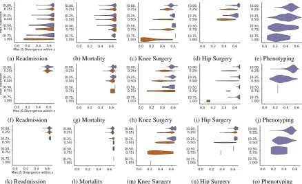
Figure 1: Median change in output ∆ ˆymed (x) densities in relation to themax attention (max ˆα)(y) ob-tained by randomly permuting instance attention weights. Colors denote classes: negative () and positive (); phenotyping (e) is not binary. Top row shows results for BiLSTM encoders; middle for CNNs; bottom for Embedding Projection.
0.0 0.2 0.4 0.6 Max JS Divergence within 0.0
0.1 0.2 0.3
0.0 0.2 0.4 0.6 Max JS Divergence within [0.00,0.25) [0.25, 0.50) [0.50, 0.75) [0.75, 1.00) Max Attention (a) Readmission
0.0 0.2 0.4 0.6 0.00 0.05 0.10 0.15 0.20 0.25
0.0 0.2 0.4 0.6 [0.00, 0.25) [0.25, 0.50) [0.50, 0.75) [0.75, 1.00) (b) Mortality
0.0 0.2 0.4 0.6 0.00 0.05 0.10 0.15 0.20 0.25
0.0 0.2 0.4 0.6 [0.00, 0.25) [0.25, 0.50) [0.50, 0.75) [0.75, 1.00)
(c) Knee Surgery
0.0 0.2 0.4 0.6 0.0
0.1 0.2 0.3 0.4
0.0 0.2 0.4 0.6 [0.00, 0.25) [0.25, 0.50) [0.50, 0.75) [0.75, 1.00)
(d) Hip Surgery
0.0 0.2 0.4 0.6 0.00
0.02 0.04 0.06 0.08
0.0 0.2 0.4 0.6 [0.00, 0.25) [0.25, 0.50) [0.50, 0.75) [0.75, 1.00) (e) Phenotyping
0.0 0.2 0.4 0.6 Max JS Divergence within 0.00 0.05 0.10 0.15 0.20 0.25
0.0 0.2 0.4 0.6 Max JS Divergence within [0.00, 0.25) [0.25, 0.50) [0.50,0.75) [0.75, 1.00) Max Attention (f) Readmission
0.0 0.2 0.4 0.6 0.0
0.1 0.2 0.3
0.0 0.2 0.4 0.6 [0.00, 0.25) [0.25, 0.50) [0.50, 0.75) [0.75, 1.00) (g) Mortality
0.0 0.2 0.4 0.6 0.00
0.05 0.10 0.15 0.20
0.0 0.2 0.4 0.6 [0.00, 0.25) [0.25, 0.50) [0.50, 0.75) [0.75, 1.00)
(h) Knee Surgery
0.0 0.2 0.4 0.6 0.0
0.2 0.4 0.6
0.0 0.2 0.4 0.6 [0.00, 0.25) [0.25, 0.50) [0.50, 0.75) [0.75, 1.00)
(i) Hip Surgery
0.0 0.2 0.4 0.6 0.000 0.025 0.050 0.075 0.100 0.125
0.0 0.2 0.4 0.6 [0.00, 0.25) [0.25, 0.50) [0.50, 0.75) [0.75, 1.00) (j) Phenotyping
0.0 0.2 0.4 0.6 Max JS Divergence within 0.0
0.1 0.2 0.3 0.4
0.0 0.2 0.4 0.6 Max JS Divergence within [0.00, 0.25) [0.25, 0.50) [0.50, 0.75) [0.75, 1.00) Max Attention (k) Readmission
0.0 0.2 0.4 0.6 0.0
0.1 0.2 0.3 0.4
0.0 0.2 0.4 0.6 [0.00,0.25) [0.25, 0.50) [0.50, 0.75) [0.75, 1.00) (l) Mortality
0.0 0.2 0.4 0.6 0.00 0.05 0.10 0.15 0.20 0.25
0.0 0.2 0.4 0.6 [0.00, 0.25) [0.25, 0.50) [0.50, 0.75) [0.75, 1.00)
(m) Knee Surgery
0.0 0.2 0.4 0.6 0.0
0.1 0.2 0.3
0.0 0.2 0.4 0.6 [0.00,0.25) [0.25, 0.50) [0.50, 0.75) [0.75, 1.00)
(n) Hip Surgery
0.0 0.2 0.4 0.6 0.000 0.025 0.050 0.075 0.100 0.125
0.0 0.2 0.4 0.6 [0.00, 0.25) [0.25, 0.50) [0.50,0.75) [0.75, 1.00) (o) Phenotyping
[image:3.595.78.517.437.705.2]Dataset Class Mean±Std. Sig. Frac. LSTM Encoder
Readmission 0 0.37±0.04 1.00
1 0.38±0.05 1.00
Mortality 0 0.33±0.05 1.00
1 0.35±0.06 1.00
Knee Surgery 0 0.38±0.07 1.00
1 0.49±0.08 1.00
Hip Surgery 0 0.24±0.07 1.00
1 0.33±0.09 1.00
Phenotyping Overall 0.24±0.06 1.00
Projection Encoder
Readmission 0 0.65±0.03 1.00
1 0.64±0.03 1.00
Mortality 0 0.76±0.02 1.00
1 0.76±0.02 1.00
Knee Surgery 0 0.65±0.05 1.00
1 0.60±0.06 1.00
Hip Surgery 0 0.59±0.09 1.00
1 0.55±0.09 1.00
[image:4.595.71.304.62.273.2]Phenotyping Overall 0.89±0.02 1.00
Table 1: Mean and std. dev. of correlations between gradient importance measures and attention weights.
Sig. Frac. columns report the fraction of instances for which this correlation is statistically significant.
4.1 Gradient Experiments
To evaluate correlations between attention weights and gradient based feature importance scores, we compute Kendall-τ measure (Table1) between at-tention scores and gradients with respect to the to-kens comprising documents. Across both corpora and all tasks we observe only a modest correla-tion between the two for BiLSTM model (the pro-jection based model have higher correspondence, which is expected for such simple architectures). This may be problematic for attention as an ex-planatory mechanism, given the explicit relation-ship between gradients and model outputs. (Al-though we note that gradient based methods them-selves pose difficulty with respect to interpretation (Feng et al.,2018)).
4.2 Counterfactual Experiments
We investigate if model predictions would have differed, had the model attended to different words (i.e., undercounterfactualattention distributions). We follow the two strategies from (Jain and Wallace,2019) for constructing counterfactual at-tention distributions. In the first we randomly per-mute the empirical weights obtained from the at-tention module prior to inducing the weighted rep-resentationhα. We repeat this process 100 times and record the median change in output.
The second strategy is adversarial; we explic-itly aim to identify attention weights that are max-imally different from the observed weights, with
Model ROC AUC PR AUC
Readmission
LR + BoW 0.70 0.29
LSTM 0.63 0.22
LSTM + Additive Attention 0.71 0.30 LSTM + Additive Attention
(Log Odds at Test) 0.69 0.26 LSTM + Log Odds Attention 0.71 0.29 Mortality
LR + BoW 0.82 0.46
LSTM 0.74 0.29
LSTM + Additive Attention 0.83 0.47 LSTM + Additive Attention
(Log Odds at Test) 0.80 0.41 LSTM + Log Odds Attention 0.82 0.42 Knee Surgery Complication
LR + BoW 0.80 0.39
LSTM 0.66 0.18
LSTM + Additive Attention 0.79 0.35 LSTM + Additive Attention
(Log Odds at Test) 0.81 0.34 LSTM + Log Odds Attention 0.81 0.38 Hip Surgery Complication
LR + BoW 0.76 0.32
LSTM 0.63 0.16
LSTM + Additive Attention 0.75 0.24 LSTM + Additive Attention
(Log Odds at Test) 0.74 0.26 LSTM + Log Odds Attention 0.78 0.29 Phenotyping
LR + BoW 0.86 0.59
LSTM 0.78 0.41
LSTM + Additive Attention 0.86 0.58 LSTM + Additive Attention
[image:4.595.306.527.63.442.2](Log Odds at Test) 0.81 0.48 LSTM + Log Odds Attention 0.85 0.56
Table 2: Predictive results across all datasets and tasks using different models and attention variants.
the constraint that this does not change the model output by more some small value. In both cases, all other model parameters are held constant.
In Figures1and2, we observe that predictions are unchanged under alternative attention config-urations in a significant majority of cases across all architectures. Thus, attention cannot be viewed casually in the sense of ‘the model made these pre-dictions because these words were attended to’. Alternative attention distributions that yield equiv-alent predictions would seem to be equally plausi-ble under the view of attention as explanation.
4.3 Log Odds Experiments
Original vs Adversarial Attention Difference :Sed dolorem sed adipisci ipsum dolor dolorem. Ut adipisci magnam tempora. Modi # eius : tempora change ipsum adipisci tempora tracheobronchomalacia quaerat dolor. Numquam est dolore labore est neque. respiratory failure Ipsum quiquia etincidunt labore modi. Dolorem aliquam dolore amet. Amet est consectetur modi neque. Porro respiratory failure etincidunt quaerat est neque dolor quaerat. Est quaerat est adipisci ipsum. Sit dolore quisquam ipsum non neque quiquia aliquam. Ut ipsum adipisci labore tempora quaerat tempora labore. Ipsum numquam voluptatem consectetur. Aliquam voluptatem , eius numquam. Velit generalized ut non numquam magnam sed modi. Consectetur porro . heart etincidunt eius consectetur , quaerat amet. Amet dolorem is difficult dolor consectetur etincidunt sed effusions quiquia aliquam. Porro etincidunt dolore labore no dolore dolorem aliquam. Tempora etincidunt quisquam aliquam numquam eius ut. tracheostomy Modi modi amet voluptatem
Original Output: 0.694Adversarial Output: 0.699
Original vs Log Odds Attention Difference : Non magnam quiquia magnam magnam quaerat. Ut etincidunt magnam voluptatem velit eius. Dolorem dolorem velit dolor porro ut etincidunt. Consectetur dolor voluptatem cystic brain mass quaerat surgical resection est magnam etincidunt. Ipsum neque dolorem sed consectetur est. Magnam modi voluptatem dolorem tempora sed ut. Dolore dolor tempora eius aliquam quisquam. Dolor quisquam eius sed labore dolore sit velit. Magnam aliquam quisquam numquam. Aliquam sed sed modi neque. Dolor chronic quiquia voluptatem adipisci quaerat adipisci. . . Magnam velit quaerat adipisci. Ut cystic brain mass adipisci velit modi. Sed aliquam astrocytoma est porro. Labore resection eius voluptatem sit quisquam consectetur modi. Est ipsum tumor dolore
[image:5.595.82.516.317.412.2]Original Output: 0.798Log Odds Output : 0.800
Figure 3: Heatmaps showing difference in Original and counterfactual attention distributions over clinical notes from MIMIC, where we have replaced text withlorem ipsumfor all but the most relevant tokens in order to preserve privacy (red implies counterfactual attention is higher and blue vice-versa). These show different cases where we can significantly change the attention distribution (eitheradversarial (Top)or usingLog Odds (Bottom)while barely affecting the prediction.
0.0 0.2 0.4 0.6 JSD (logodds vs normal) [0.00,
0.25) [0.25, 0.50) [0.50, 0.75) [0.75, 1.00)
Max Attention
0.0 0.2 0.4 0.6 JSD (logodds vs normal) 0.0
0.2 0.4 0.6 0.8 1.0
Output Difference
(a) Readmission
0.0 0.2 0.4 0.6 [0.00,
0.25) [0.25, 0.50) [0.50, 0.75) [0.75, 1.00)
0.0 0.2 0.4 0.6 0.0
0.2 0.4 0.6 0.8 1.0
(b) Mortality
0.0 0.2 0.4 0.6 [0.00,
0.25) [0.25, 0.50) [0.50, 0.75) [0.75, 1.00)
0.0 0.2 0.4 0.6 0.0
0.2 0.4 0.6 0.8 1.0
(c) Knee Surgery
0.0 0.2 0.4 0.6 [0.00,
0.25) [0.25, 0.50) [0.50, 0.75) [0.75, 1.00)
0.0 0.2 0.4 0.6 0.0
0.2 0.4 0.6 0.8 1.0
(d) Hip Surgery
0.0 0.2 0.4 0.6 [0.00,
0.25) [0.25, 0.50) [0.50, 0.75) [0.75, 1.00)
0.0 0.2 0.4 0.6 0.0
0.2 0.4 0.6 0.8 1.0
(e) Phenotyping
Figure 4: Change in output (y-axis) using original attention vs Log Odds attention during predictions against JSD between these two distributions (x-axis). These results are for LSTM encoders.
the word present at each position and passing this through a softmax: αLO = softmaxt({βwt}
T
t=1)
wherewtis the word at positiontandβ are log-odds estimates.
These scores enjoy a clear interpretation under a linear regime. We thus explore two ways of using them with attentive neural models: (1) Swapping in these in as attention weights place ofhαat test (prediction) time; (2) Use the (fixed) ‘log-odds at-tention’ during training, in place of learning the attention distribution end-to-end.
Table 2 shows that using log odds attention at test time does not degrade the performance sig-nificantly in most datasets (and actually improves performance for the Knee Surgery Complications task). Similarly, using log odds attention during training also yields similar performance to stan-dard attention variants. But as we see in Figure4, log odds attention distributions can differ consid-erably from learned attention distributions, again highlighting the difficulty of interpreting attention weights.
5 Discussion and Conclusions
Across two EMR datasets and five predictive tasks, we have shown that (i) attention mech-anisms substantially boost the performance of LSTM text encoders passed over clinical notes, but, (ii) treating attention weights as ‘explana-tions’ for predictions is unwarranted. The latter confirms that the recent general findings of (Jain and Wallace, 2019) hold in the clinical domain; this is important because interpretability in this space is critical for obvious reasons.
We hope that this paper inspires work on trans-parent attention mechanisms for models that make predictions on the basis of EMR.
Acknowledgments
References
Dzmitry Bahdanau, Kyunghyun Cho, and Yoshua Ben-gio. 2014. Neural machine translation by jointly learning to align and translate. arXiv preprint arXiv:1409.0473.
Willie Boag, Dustin Doss, Tristan Naumann, and Pe-ter Szolovits. 2018. What‘s in a note? unpack-ing predictive value in clinical note representations.
AMIA Summits on Translational Science Proceed-ings, 2017:26.
Shi Feng, Eric Wallace, Alvin Grissom II, Pedro Rodriguez, Mohit Iyyer, and Jordan Boyd-Graber. 2018. Pathologies of neural models make interpreta-tion difficult. InEmpirical Methods in Natural Lan-guage Processing.
Marzyeh Ghassemi, Tristan Naumann, Finale Doshi-Velez, Nicole Brimmer, Rohit Joshi, Anna Rumshisky, and Peter Szolovits. 2014. Unfolding physiological state: Mortality modelling in inten-sive care units. In Proceedings of the 20th ACM SIGKDD international conference on Knowledge discovery and data mining, pages 75–84. ACM.
Hrayr Harutyunyan, Hrant Khachatrian, David C Kale, and Aram Galstyan. 2017. Multitask learning and benchmarking with clinical time series data. arXiv preprint arXiv:1703.07771.
Sarthak Jain and Byron C Wallace. 2019. Attention is not explanation. arXiv preprint arXiv:1902.10186.
Mengqi Jin, Mohammad Taha Bahadori, Aaron Co-lak, Parminder Bhatia, Busra Celikkaya, Ram Bhakta, Selvan Senthivel, Mohammed Khalilia, Daniel Navarro, Borui Zhang, et al. 2018. Im-proving hospital mortality prediction with medical named entities and multimodal learning. arXiv preprint arXiv:1811.12276.
Alistair EW Johnson, Tom J Pollard, Lu Shen, H Lehman Li-wei, Mengling Feng, Moham-mad Ghassemi, Benjamin Moody, Peter Szolovits, Leo Anthony Celi, and Roger G Mark. 2016. Mimic-iii, a freely accessible critical care database.
Scientific data, 3:160035.
Jiwei Li, Will Monroe, and Dan Jurafsky. 2016. Un-derstanding neural networks through representation erasure. arXiv preprint arXiv:1612.08220.
Yu-Wei Lin, Yuqian Zhou, Faraz Faghri, Michael J Shaw, and Roy H Campbell. 2018. Analysis and prediction of unplanned intensive care unit read-mission using recurrent neural networks with long short-term memory.bioRxiv.
Zachary C Lipton, David C Kale, Charles Elkan, and Randall Wetzel. 2015. Learning to diagnose with lstm recurrent neural networks. arXiv preprint arXiv:1511.03677.
Sampo Pyysalo, Filip Ginter, Hans Moen, Tapio Salakoski, and Sophia Ananiadou. 2013. Distribu-tional semantics resources for biomedical text pro-cessing.Proceedings of LBM, pages 39–44.
Andrew Slavin Ross, Michael C Hughes, and Finale Doshi-Velez. 2017. Right for the right reasons: Training differentiable models by constraining their explanations. arXiv preprint arXiv:1703.03717.
An Analysis of Attention over Clinical Notes for Predictive Tasks:
Appendix
A Dataset Statistics
Task |V| Avg. length Train size Test size
Readmission 36464 3865 23790 / 5499 4265 / 735
Mortality 34030 3901 21347 / 4675 4323 / 677
Hip Surgery Complications 10842 2624 3281 / 369 719 / 75 Knee Surgery Complications 10842 2586 2664 / 324 582 / 48
Phenotyping 10842 3641 31075 5000
Table 3: Dataset characteristics. For train and test size, we list the cardinality for each class, where applicable:0/1 for binary classification and overall for multilabel. Average length is in tokens.
The Phenotypes studied in Phenotyping task are
-Acute and unspecified renal failure, -Acute cerebrovascular disease, -Acute myocardial infarction, Car-diac dysrhythmias, Chronic kidney disease, Chronic obstructive pulmonary disease and bronchiectasis, Complications of surgical procedures or medical care, Conduction disorders, Congestive heart failure - nonhypertensive, Coronary atherosclerosis and other heart disease, Diabetes mellitus with complica-tions, Diabetes mellitus without complication, Disorders of lipid metabolism, Essential hypertension, Fluid and electrolyte disorders, Gastrointestinal hemorrhage, Hypertension with complications and sec-ondary hypertension, Other liver diseases, Other lower respiratory disease, Other upper respiratory dis-ease, Pleurisy - pneumothorax - pulmonary collapse, Pneumonia (except that caused by tuberculosis or sexually transmitted disease), Respiratory failure - insufficiency - arrest (adult), Septicemia (except in labor), Shock .
B Model Details
For all datasets, we usespaCyfor tokenization. We map out of vocabulary words to a special<unk> token and map any word with numeric characters to ‘qqq’. Each word in the vocabulary was initialized using pretrained embeddings (Pyysalo et al.,2013). We initialize words not present in the vocabulary using samples from a standard Gaussian (µ= 0,σ2= 1).
B.1 BiLSTM
We use an embedding size of 300 and hidden size of 128 for all datasets. The model was regularized withL2 regularization (λ= 10−5) applied to all parameters. We use a sigmoid activation function for all binary classification tasks. We treat each phenotype classification as binary classification and take the mean loss over labels during training. We trained the model using maximum likelihood loss function with Adam Optimizer with default parameters in PyTorch.
B.2 CNN
We use an embedding size of 300 and 4 kernels of sizes [1, 3, 5, 7], each with 64 filters, giving a final hidden size of 256. We use ReLU activation function on the output of the filters. All other configurations remain same as BiLSTM.
B.3 Average