Learning to Explicitate Connectives with Seq2Seq Network
for Implicit Discourse Relation Classification
Wei Shi†and Vera Demberg†,‡ †
Dept. of Language Science and Technology ‡
Dept. of Mathematics and Computer Science, Saarland University Saarland Informatics Campus, 66123 Saarbr¨ucken, Germany
{w.shi, vera}@coli.uni-saarland.de
Abstract
Implicit discourse relation classification is one of the most difficult steps in discourse parsing. The difficulty stems from the fact that the coherence relation must be inferred based on the content of the discourse relational arguments. Therefore, an effective encoding of the relational arguments is of crucial importance. We here propose a new model for implicit discourse relation classification, which consists of a classifier, and a sequence-to-sequence model which is trained to generate a repre-sentation of the discourse relational arguments by trying to predict the relational arguments including a suitable implicit connective. Training is possible because such implicit connectives have been an-notated as part of the PDTB corpus. Along with a memory network, our model could generate more refined representations for the task. And on the now standard 11-way classification, our method out-performs the previous state of the art systems on the PDTB benchmark on multiple settings including cross validation.
1
Introduction
Discourse relations describe the logical relation between two sentences/clauses. When understanding a text, humans infer discourse relation between text segmentations. They reveal the structural organization of text, and allow for additional inferences. Many natural language processing tasks, such as machine translation, question-answering, automatic summarization, sentiment analysis, and sentence embedding learning, can also profit from having access to discourse relation information. Recent years have seen more and more works on this topic, including two CoNNL shared tasks (Xue et al., 2015, 2016).
Penn Discourse Tree Bank (Prasad et al., 2008, PDTB) provides lexically-grounded annotations of discourse relations and their two discourse relational arguments (i.e., two text spans). Discourse relations are sometimes signaled by explicit discourse markers (e.g.,because, but). Example 1 shows an explicit discourse relation marked by “because”; the presence of the connective makes it possible to classify the discourse relation with high reliability: Miltsakaki et al. (2005) reported an accuracy of 93.09% for 4-way classification of explicits.
1. [I refused to pay the cobbler the full $95]Arg1because[He did poor work.]Arg2
— Explicit, Contingency.Cause
2. [In the energy mix of the future, bio-energy will also have a key role to play in boosting rural employment and the rural economy in Europe .]Arg1(Implicit = However) [At the same time , the promotion of
bio-energy must not lead to distortions of competition.]Arg2
— Implicit, Comparison.Contrast
The key in implicit discourse relation classification lies in extracting relevant information for the relation label from (the combination of) the discourse relational arguments. Informative signals can consist of surface cues, as well as the semantics of the relational arguments. Statistical approaches have typically relied on linguistically informed features which capture both of these aspects, like temporal markers, polarity tags, Levin verb classes and sentiment lexicons, as well as the Cartesian products of the word tokens in the two arguments (Lin et al., 2009). More recent efforts use distributed representations with neural network architectures (Qin et al., 2016a).
The main question in designing neural networks for discourse relation classification is how to get the neural networks to effectively encode the discourse relational arguments such that all of the aspects rele-vant to the classification of the relation are represented, in particular in the face of very limited amounts of annotated training data, see e.g. Rutherford et al. (2017). The crucial intuition in the present paper is to make use of the annotated implicit connectives in the PDTB: in addition to the typical relation label classification task, we also train the model to encode and decode the discourse relational arguments, and at the same time predict the implicit connective. This novel secondary task forces the internal represen-tation to more completely encode the semantics of the relational arguments (in order to allow the model to decode later), and to make a more fine-grained classification (predicting the implicit connective) than is necessary for the overall task. This more fine-grained task thus aims to force the model to represent the discourse relational arguments in a way that allows the model to also predict a suitable connective. Our overall discourse relation classifier combines representations from the relational arguments as well as the hidden representations generated as part of the encoder-decoder architecture to predict relation labels. What’s more, with an explicit memory network, the network also has access to history represen-tations and acquire more explicit context knowledge. We show that our method outperforms previous approaches on the 11-way classification on the PDTB 2.0 benchmark.
The remaining of the paper is organized as follows: Section 2 discusses related work; Section 3 describes our proposed method; Section 4 gives the training details and experimental results, which is followed by conclusion and future work in section 5.
2
Related Work
2.1 Implicit Discourse Relation Classification
Implicit discourse relation recognition is one of the most important components in discourse parsing. With the release of PDTB (Prasad et al., 2008), the largest available corpus which annotates implicit examples with discourse relation labels and implicit connectives, a lot of previous works focused on typical statistical machine learning solutions with manually crafted sparse features (Rutherford and Xue, 2014).
Recently, neural networks have shown an advantage of dealing with data sparsity problem, and many deep learning methods have been proposed for discourse parsing, including convolutional (Zhang et al., 2015), recurrent (Ji et al., 2016), character-based (Qin et al., 2016a), adversarial (Qin et al., 2017) neural networks, and pair-aware neural sentence modeling (Cai and Zhao, 2017). Multi-task learning has also been shown to be beneficial on this task (Lan et al., 2017).
cn
c1 Softmax
Global Attention
…
w1 w2 w3 wn-1 wn
… …
…
y1 y2
<sos> yn-1 yn
…
α1 y1
…
y2 <eos>
Gated-Interaction Layer
…
…
En
co
de
r
Context Vector
Decoder y3 yn
Softmax Layer Classifier
ˆ hd
he
h1d
hn d
… αn
h* Knowledge Vector Attention
Update
Context Memory
[image:3.595.140.453.71.275.2]…
Figure 1: The Architecture of Proposed Model.
the text in the target language which were not originally present in the source language. They used ex-plicitated connectives as a source of weak supervision to obtain additional labeled instances, and showed that this extension of the training data leads to substantial performance improvements.
The huge gap between explicit and implicit relation recognition (namely, 50% vs. 90% in 4-way classification) also motivates to incorporate connective information to guide the reasoning process. Zhou et al. (2010) used a language model to automatically insert discourse connectives and leverage the infor-mation of these predicted connectives. The approach which is most similar in spirit to ours, Qin et al. (2017), proposed a neural method that incorporates implicit connectives in an adversarial framework to make the representation as similar as connective-augmented one and showed that the inclusion of implicit connectives could help to improve classifier performance.
2.2 Sequence-to-sequence Neural Networks
Sequence to sequence model is a general end-to-end approach to sequence learning that makes minimal assumptions on the sequence structure, and firstly proposed by Sutskever et al. (2014). It uses multi-layered Long Short-Term Memory (LSTM) or Gated Recurrent Units (GRU) to map the input sequence to a vector with a fixed dimensionality, and then decode the target sequence from the vector with another LSTM / GRU layer.
Sequence to sequence models allow for flexible input/output dynamics and have enjoyed great suc-cess in machine translation and have been broadly used in variety of sequence related tasks such as Question Answering, named entity recognition (NER) / part of speech (POS) tagging and so on.
If the source and target of a sequence-to-sequence model are exactly the same, it is also called Auto-encoder, Dai and Le (2015) used a sequence auto-encoder to better represent sentence in an unsupervised way and showed impressive performances on different tasks. The main difference between our model and this one is that we have different input and output (the output contains a connective while the input doesn’t). In this way, the model is forced to explicitate implicit relation and try to learn the latent pattern and discourse relation between implicit arguments and connectives and then generate more discriminative representations.
3
Methodology
consists of three components: Encoder, Decoder and Discourse Relation Classifier. We here use different LSTMs for the encoding and decoding tasks to help keep the independence between those two parts.
The task of implicit discourse relation recognition is to recognize the senses of the implicit relations, given the two arguments. For each discourse relation instance, The Penn Discourse Tree Bank (PDTB) provides two arguments (Arg1, Arg2) along with the discourse relation (Rel) and manually inserted
implicit discourse connective (Conni). Here is an implicit example from section 0 in PDTB:
3. Arg1: This is an old story.
Arg2: We’re talking about years ago before anyone heard of asbestos having any questionable properties. Conni: in fact
Rel: Expansion.Restatement
During training, the input and target sentences for sequence-to-sequence neural network are[Arg1;Arg2]
and[Arg1;Conni;Arg2]respectively, where “;” denotes concatenation.
3.1 Model Architecture
3.1.1 Encoder
Given a sequence of words, an encoder computes a joint representation of the whole sequence.
After mapping tokens to Word2Vec embedding vectors (Mikolov et al., 2013), a LSTM recurrent neural network processes a variable-length sequencex = (x1, x2, ..., xn). At time step t, the state of memory cellctand hiddenhtare calculated with the Equations 1:
it
ft
ot
ˆ
ct
=
σ σ σ tanh
W ·[ht−1, xt]
ct=ftct−1+itcˆt
ht=ottanh(ct)
(1)
wherextis the input at time stept,i,f andoare the input, forget and output gate activation respec-tively. ctˆ denotes the current cell state, σ is the logistic sigmoid function and denotes element-wise multiplication. The LSTM separates the memory c from the hidden state h, which allows for more flexibility incombining new inputs and previous context.
For the sequence modeling tasks, it is beneficial to have access to the past context as well as the future context. Therefore, we chose a bidirectional LSTM as the encoder and the output of the word at time-step tis shown in the Equation 2. Here, element-wise sum is used to combine the forward and backward pass outputs.
ht=
h−→
ht⊕
←−
ht
i
(2)
Thus we get the output of encoder:
he= [he1, h
e
2, ..., h
e
n] (3)
3.1.2 Decoder
With the representation from the encoder, the decoder tries to map it back to the targets space and predicts the next words.
Here we used a separate LSTM recurrent network to predict the target words. During training, target words are fed into the LSTM incrementally and we get the outputs from decoder LSTM:
hd=
hd1, hd2, ..., hdn
Global Attention
In each time-step in decoding, it’s better to consider all the hidden states of the encoder to give the decoder a full view of the source context. So we adopted the global attention mechanism proposed in Luong et al. (2015). For time steptin decoding, context vector ctis the weighted average of he, the weights for each time-step are calculated withhdt andheas illustrated below:
αt=
exp(hd
t
>
Wαhe)
n P t=1
exp(hd
t
>
Wαhe)
(5)
ct=αhe (6)
Word Prediction
Context vectorctcaptured the relevant source side information to help predict the current target wordyt. We employ a concatenate layer with activation functiontanhto combine context vectorctand hidden state of decoderhd
t at time-step t as follows:
ˆ
hd
t = tanh(Wc
ct;hdt
) (7)
Then the predictive vector is fed into the softmax layer to get the predicted distribution pˆ(yt|s) of the current target word.
ˆ
p(yt|s) =sof tmax(Wshˆd+bs)
ˆ
yt= arg max
y pˆ(yt|s)
(8)
After decoding, we obtain the predictive vectors for the whole target sequence hˆd =
hd1, hd2, ..., hdn. Ideally, it contains the information of exposed implicit connectives.
Gated Interaction
In order to predict the coherent discourse relation of the input sequence, we take both thehencoder and the predictive word vectorshdinto account. K-max pooling can “draw together” features that are most discriminative and among many positions apart in the sentences, especially on both the two relational arguments in our task here; this method has been proved to be effective in choosing active features in sentence modeling (Kalchbrenner et al., 2014). We employ an average k-max pooling layer which takes average of the top k-max values among the whole time-steps as in Equation 9 and 10:
¯
he=
1 k
k X
i=1
topk(he) (9)
¯
hd=
1 k
k X
i=1
topk( ˆhd) (10)
¯
heand¯hdare then combined using a linear layer (Lan et al., 2017). As illustrated in Equation 11, the linear layer acts as a gate to determine how much information from the sequence-to-sequence network should be mixed into the original sentence’s representations from the encoder. Compared with bilinear layer, it also has less parameters and allows us to use high dimensional word vectors.
h∗= ¯he⊕σ(Wi¯hd+bi) (11)
Explicit Context Knowledge
Given a representationh∗ from the interaction layer, we generate aknowledge vector by weighted memory reading:
k=M sof tmax(MTh∗) (12)
We here use dot product attention, which is faster and space-efficient than additive attention, to calculate the scores for each training instances. The scores are normalized with a softmax layer and the final knowledge vector is a weighted sum of the columns in memory matrixM.
Afterwards, the model predicts the discourse relation using a softmax layer.
ˆ
p(r|s) =sof tmax(Wr[k;h∗] +br)
ˆ
r= arg max
y pˆ(r|s)
(13)
3.2 Multi-objectives
In our model, the decoder and the discourse relation classifier have different objectives. For the decoder, the objective consists of predicting the target word at each time-step. The loss function is calculated with masked cross entropy withL2regularization, as follows:
Lossde =−
1 n
n X
t=1
ytlog( ˆpy) +
λ
2 kθdek
2
2 (14)
whereytis one-hot represented ground truth of target words, pˆy is the estimated probabilities for each words in vocabulary by softmax layer,ndenotes the length of target sentence.λis a hyper-parameter of L2regularization andθis the parameter set.
The objective of the discourse relation classifier consists of predicting the discourse relations. A rea-sonable training objective for multiple classes is the categorical cross-entropy loss. The loss is formulated as:
Losscl=−
1 m
m X
i=1
rilog( ˆpr) +
λ
2 kθclk
2
2 (15)
whereriis one-hot represented ground truth of discourse relation labels,pˆrdenotes the predicted prob-abilities for each relation class by softmax layer,mis the number of target classes. Just like above,λis a hyper-parameter ofL2regularization.
For the overall loss of the whole model, we set another hyper-parameterwto give these two objective functions different weights. Largerwmeans that more importance is placed on the decoder task.
Loss =w·Lossde+ (1−w)·Losscl (16)
3.3 Model Training
To train our model, the training objective is defined by the loss function we introduced above. We use Adaptive Moment Estimation (Adam) (Kingma and Ba, 2014) with different learning rate for different parts of the model as our optimizer. Dropout layers are applied after the embedding layer and also on the top feature vector before the softmax layer in the classifier. We also employL2regularization with small
λin our objective functions for preventing over-fitting. The values of the hyper-parameters, are provided in Table 2. The model is trained firstly to minimize the loss in Equation 14 until convergence, we use scheduled sampling (Bengio et al., 2015) during training to avoid “teacher-forcing problem”. And then to minimize the joint loss in Equation 16 to train the implicit discourse relation classifier.
4
Experiments and Results
4.1 Experimental Setup
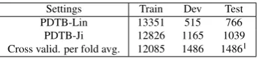
Settings Train Dev Test
PDTB-Lin 13351 515 766
PDTB-Ji 12826 1165 1039
[image:7.595.206.392.69.111.2]Cross valid. per fold avg. 12085 1486 14861
Table 1: Numbers of train, development and test set on different settings for 11-way classification task. Instances annotated with two labels are double-counted and some relations with few instances have been removed.
works we directly compare to in our evaluation, we here use the setting where AltLex, EntRel and NoRel tags are ignored. About 2.2% of the implicit relation instances in PDTB have been annotated with two relations, these are considered as two training instances.
To allow for full comparability to earlier work, we here report results for three different settings. The first one is denoted as PDTB-Lin (Lin et al., 2009); it uses sections 2-21 for training, 22 as dev and section 23 as test set. The second one is labeled PDTB-Ji (Ji and Eisenstein, 2015), and uses sections 2-20 for training, 0-1 as dev and evaluates on sections 21-22. Our third setting follows the recommendations of Shi and Demberg (2017), and performs 10-fold cross validation on the whole corpus (sections 0-23). Table 1 shows the number of instances in train, development and test set in different settings.
The advantage of the cross validation approach is that it addresses problems related to the small cor-pus size, as it reports model performance across all folds. This is important, because the most frequently used test set (PDTB-Lin) contains less than 800 instances; taken together with a lack in the community to report mean and standard deviations from multiple runs of neural networks (Reimers and Gurevych, 2018), the small size of the test set makes reported results potentially unreliable.
Preprocessing
We first convert tokens in PDTB to lowercase and normalize strings, which removes special characters. The word embeddings used for initializing the word representations are trained with the CBOW archi-tecture in Word2Vec2 (Mikolov et al., 2013) on PDTB training set. All the weights in the model are initialized with uniform random.
To better locate the connective positions in the target side, we use two position indicators (hconni, h/conni) which specify the starting and ending of the connectives (Zhou et al., 2016), which also indicate the spans of discourse arguments.
Since our main task here is not generating arguments, it is better to have representations generated by correct words rather than by wrongly predicted ones. So at test time, instead of using the predicted word from previous time step as current input, we use the source sentence as the decoder’s input and target. As the implicit connective is not available at test time, we use a random vector, which we used as “impl conn” in Figure 2, as a placeholder to inform the sequence that the upcoming word should be a connective.
Hyper-parameters
There are several hyper-parameters in our model, including dimension of word vectorsd, two dropout rates after embedding layerq1 and before softmax layerq2, two learning rates for encoder-decoderlr1
and for classifierlr2, topkfor k-max pooling layer, different weightswfor losses in Equation (16) andλ
denotes the coefficient of regularizer, which controls the importance of the regularization term, as shown in Table 2.
1Cross-validation allows us to test on all 15057 instances.
2
https://code.google.com/archive/p/word2vec/
d q1 q2 lr1 lr2 k w λ
100 0.5 0.2 2.5e−3 5e−3 5 0.2 5e−4
Methods PDTB-Lin PDTB-Ji Cross Validation
Majority class 26.11 26.18 25.59
Lin et al. (2009) 40.20 -
-Qin et al. (2016a) 43.81 45.04
-Cai and Zhao (2017) - 45.81
-Qin et al. (2017) 44.65 46.23
-Shi et al. (2017) (with extra data) 45.50 - 37.84
Encoder only (Bi-LSTM) (Shi et al., 2017) 34.32 - 30.01
Auto-Encoder 43.86 45.43 39.50
Seq2Seq w/o Mem Net 45.75 47.05 40.29
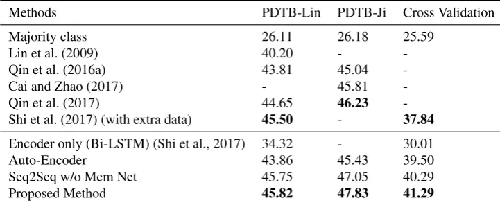
[image:8.595.116.477.71.219.2]Proposed Method 45.82 47.83 41.29
Table 3: Accuracy (%) of implicit discourse relations on PDTB-Lin, PDTB-Ji and Cross Validation Settings for multi-class classification.
4.2 Experimental Results
We compare our models with six previous methods, as shown in Table 3. The baselines contain feature-based methods (Lin et al., 2009), state-of-the-art neural networks (Qin et al., 2016a; Cai and Zhao, 2017), including the adversarial neural network that also exploits the annotated implicit connectives (Qin et al., 2017), as well as the data extension method based on using explicitated connectives from translation to other languages (Shi et al., 2017).
Additionally, we ablate our model by taking out the prediction of the implicit connective in the sequence to sequence model. The resulting model is labeled Auto-Encoder in Table 3. And seq2seq network without knowledge memory, which means we use the output of gated interaction layer to predict the label directly, as denoted as Seq2Seq w/o Mem Net.
Our proposed model outperforms the other models in each of the settings. Compared with perfor-mances in Qin et al. (2017), although we share the similar idea of extracting highly discriminative fea-tures by generating connective-augmented representations for implicit discourse relations, our method improves about 1.2% on setting PDTB-Lin and 1.6% on the PDTB-Ji setting. The importance of the implicit connective is also illustrated by the fact that the “Auto-Encoder” model, which is identical to our model except it does not predict the implicit connective, performs worse than the model which does. This confirms our initial hypothesis that training with implicit connectives helps to expose the latent discrim-inative features in the relational arguments, and generates more refined semantic representation. It also means that, to some extent, purely increasing the size of tunable parameters is not always helpful in this task and trying to predict implicit connectives in the decoder does indeed help the model extract more discriminative features for this task. What’s more, we can also see that without the memory network, the performances are also worse, it shows that with the concatenation of knowledge vector, the training instance may be capable of finding related instances to get common knowledge for predicting implicit relations. As Shi and Demberg (2017) argued that it is risky to conclude with testing on such small test set, we also run cross-validation on the whole PDTB. From Table 3, we have the same conclusion with the effectiveness of our method, which outperformed the baseline (Bi-LSTM) with more than 11% points and 3% compared with Shi et al. (2017) even though they have used a very large extra corpus.
For the sake of obtaining a better intuition on how the global attention works in our model, Figure 2 demonstrates the weights of different time-steps in attention layer from the decoder. The weights show how much importance the word attached to the source words while predicting target words. We can see that without the connective in the target side of test, the word filler still works as a connective to help predict the upcoming words. For instance, the true discourse relation for the right-hand example is
Figure 2: Visualization of attention weights during predicting target sentence in train and test, x-axis denotes the source sentence and the y-axis is the targets. First two figures are examples from training set with implicit connectives inside, while the following one, in which the implicit connective has been replaced by the word filler “impl conn”, is from test.
In recent years, U.S. steelmakers have supplied about 80% of the 100 million tons of steel used annually by the nation. (in
addition,) Of the remaining 20% needed, the steel-quota negotiations allocate about 15% to foreign suppliers.
— Expansion.Conjunction
1. The average debt of medical school graduates who borrowed to pay for their education jumped 10% to $42,374 this year from $38,489 in 1988, says the Association of American Medical Colleges. (furthermore) that’s 115% more than in 1981 — Expansion.Conjunction 2. ... he rigged up an alarm system, including a portable beeper, to alert him when Sventek came on the line. (and) Some nights he slept under his desk.
— Expansion.Conjunction
Prices for capital equipment rose a hefty 1.1% in September, while prices for home electronic equipment fell 1.1%. (
Mean-while,) food prices declined 0.6%, after climbing 0.3% in August.
— Comparison.Contrast
1. Lloyd’s overblown bureaucracy also hampers efforts to update marketing strategies. (Although) some underwriters have been pressing for years to tap the low-margin business by selling some policies directly to consumers.
— Comparison.Contrast 2. Valley National ”isn’t out of the woods yet. (Specifically), the key will be whether Arizona real estate turns around or at least stabilizes
[image:9.595.215.383.565.640.2]— Expansion.Restatement
Table 4: Example of attention in Context Knowledge Memory. The sentences in italic are from PDTB test set and following 2 instances are the ones with top 2 attention weights from training set.
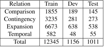
Relation Train Dev Test Comparison 1855 189 145 Contingency 3235 281 273 Expansion 6673 638 538
Temporal 582 48 55
Total 12345 1156 1011
Table 5: Distribution of top-level implicit discourse relations in the PDTB.
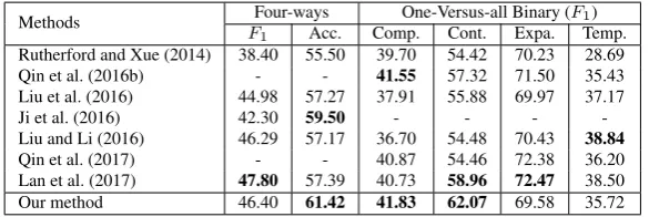
Methods Four-ways One-Versus-all Binary (F1)
F1 Acc. Comp. Cont. Expa. Temp.
Rutherford and Xue (2014) 38.40 55.50 39.70 54.42 70.23 28.69 Qin et al. (2016b) - - 41.55 57.32 71.50 35.43 Liu et al. (2016) 44.98 57.27 37.91 55.88 69.97 37.17
Ji et al. (2016) 42.30 59.50 - - -
-Liu and Li (2016) 46.29 57.17 36.70 54.48 70.43 38.84
[image:10.595.152.445.70.168.2]Qin et al. (2017) - - 40.87 54.46 72.38 36.20 Lan et al. (2017) 47.80 57.39 40.73 58.96 72.47 38.50 Our method 46.40 61.42 41.83 62.07 69.58 35.72
Table 6: Comparison ofF1scores (%) and Accuracy (%) with the State-of-the-art Approaches for
four-ways and one-versus-all binary classification on PDTB. Comp., Cont., Expa. and Temp. stand for Comparison, Contingency, Expansion and Temporal respectively.
4.2.1 Top-level Binary and 4-way Classification
A lot of the recent works in PDTB relation recognition have focused on first level relations, both on binary and 4-ways classification. We also report the performance on level-one relation classification for more comparison to prior works. As described above, we followed the conventional experimental settings (Rutherford and Xue, 2015; Liu and Li, 2016) as closely as possible. Table 5 shows the distribution of top-level implicit discourse relation in PDTB, it’s worth noticing that there are only 55 instances for Temporal Relation in the test set.
To make the results comparable with previous work, we report theF1score for four binary
classifi-cations and bothF1 and Accuracy for 4-way classification, which can be found in Table 6. We can see
that our method outperforms all alternatives on COMPARISONand CONTINGENCY, and obtain compa-rable scores with the state-of-the-art in others. For 4-way classification, we got the best accuracy and second-bestF1with around 2% better than in Ji et al. (2016).
5
Conclusion and Future Work
We present in this paper a novel neural method trying to integrate implicit connectives into the represen-tation of implicit discourse relations with a joint learning framework of sequence-to-sequence network. We conduct experiments with different settings on PDTB benchmark, the results show that our proposed method can achieve state-of-the-art performance on recognizing the implicit discourse relations and the improvements are not only brought by the increasing number of parameters. The model also has great potential abilities in implicit connective prediction in the future.
Our proposed method shares similar spirit with previous work in Zhou et al. (2010), who also tried to leverage implicit connectives to help extract discriminative features from implicit discourse instances. Comparing with the adversarial method proposed by Qin et al. (2017), our proposed model more closely mimics humans’ annotation process of implicit discourse relations and is trained to directly explicitate the implicit relations before classification. With the representation of the original implicit sentence and the explicitated one from decoder, and the help of the explicit knowledge vector from memory network, the implicit relation could be classified with higher accuracy.
Although our method has not been trained as a generative model in our experiments, we can see potential for applying it to generative tasks. With more annotated data, minor modification and fine-tuned training, we believe our proposed method could also be applied to tasks like implicit discourse connective prediction, or argument generation in the future.
6
Acknowledgments
References
Bengio, S., O. Vinyals, N. Jaitly, and N. Shazeer (2015). Scheduled sampling for sequence prediction with recurrent neural networks. InProceeding of NIPS, pp. 1171–1179.
Cai, D. and H. Zhao (2017). Pair-aware neural sentence modeling for implicit discourse relation classi-fication. InIEA-AIE, pp. 458–466. Springer.
Dai, A. M. and Q. V. Le (2015). Semi-supervised sequence learning. In Proceedings of NIPS, pp. 3079–3087.
Hochreiter, S. and J. Schmidhuber (1997). Long short-term memory. Neural computation 9(8), 1735– 1780.
Ji, Y. and J. Eisenstein (2015). One vector is not enough: Entity-augmented distributional semantics for discourse relations. TACL 3, 329–344.
Ji, Y., G. Haffari, and J. Eisenstein (2016). A latent variable recurrent neural network for discourse relation language models. InProceedings of NAACL, pp. 332–342.
Kalchbrenner, N., E. Grefenstette, and P. Blunsom (2014). A convolutional neural network for modelling sentences. InProceedings of ACL.
Kingma, D. and J. Ba (2014). Adam: A method for stochastic optimization. arXiv preprint arXiv:1412.6980.
Lan, M., J. Wang, Y. Wu, Z.-Y. Niu, and H. Wang (2017). Multi-task attention-based neural networks for implicit discourse relationship representation and identification. InProceedings of EMNLP, pp. 1299–1308.
Lin, Z., M.-Y. Kan, and H. T. Ng (2009). Recognizing implicit discourse relations in the penn discourse treebank. InProceedings of EMNLP, pp. 343–351.
Liu, Q., Y. Zhang, and J. Liu (2018). Learning domain representation for multi-domain sentiment clas-sification. InProceedings of NAACL, pp. 541–550.
Liu, Y. and S. Li (2016). Recognizing implicit discourse relations via repeated reading: Neural networks with multi-level attention. InProceedings of EMNLP, pp. 1224–1233.
Liu, Y., S. Li, X. Zhang, and Z. Sui (2016). Implicit discourse relation classification via multi-task neural networks. InProceedings of AAAI, pp. 2750–2756.
Luong, M.-T., H. Pham, and C. D. Manning (2015). Effective approaches to attention-based neural machine translation. InProceedings of EMNLP, pp. 1412–1421.
Mikolov, T., I. Sutskever, K. Chen, G. S. Corrado, and J. Dean (2013). Distributed representations of words and phrases and their compositionality. InProceedings of NIPS, pp. 3111–3119.
Miltsakaki, E., N. Dinesh, R. Prasad, A. Joshi, and B. Webber (2005). Experiments on sense annotations and sense disambiguation of discourse connectives. InProceedings of the Fourth Workshop TLT-2005.
Prasad, R., N. Dinesh, A. Lee, E. Miltsakaki, L. Robaldo, A. Joshi, and B. Webber (2008). The penn discourse treebank 2.0. InProceedings of LREC.
Qin, L., Z. Zhang, and H. Zhao (2016a). Implicit discourse relation recognition with context-aware character-enhanced embeddings. InProceedings of COLING.
Qin, L., Z. Zhang, H. Zhao, Z. Hu, and E. Xing (2017). Adversarial connective-exploiting networks for implicit discourse relation classification. InProceedings of ACL, pp. 1006–1017.
Reimers, N. and I. Gurevych (2018). Why comparing single performance scores does not allow to draw conclusions about machine learning approaches.arXiv preprint arXiv:1803.09578.
Rutherford, A., V. Demberg, and N. Xue (2017). A systematic study of neural discourse models for implicit discourse relation. InProceedings of EACL, pp. 281–291.
Rutherford, A. and N. Xue (2014). Discovering implicit discourse relations through brown cluster pair representation and coreference patterns. InProceedings of EACL, pp. 645–654.
Rutherford, A. and N. Xue (2015). Improving the inference of implicit discourse relations via classifying explicit discourse connectives. InProceedings of NAACL, pp. 799–808.
Shi, W. and V. Demberg (2017). On the need of cross validation for discourse relation classification. In
Proceedings of EACL, pp. 150–156.
Shi, W., F. Yung, and V. Demberg (2018). Acquiring annotated data with cross-lingual explicitation for implicit discourse relation classification.arXiv preprint arXiv:1808.10290.
Shi, W., F. Yung, R. Rubino, and V. Demberg (2017). Using explicit discourse connectives in translation for implicit discourse relation classification. InProceedings of IJCNLP, pp. 484–495.
Sutskever, I., O. Vinyals, and Q. V. Le (2014). Sequence to sequence learning with neural networks. In
Proceedings of NIPS, pp. 3104–3112.
Wu, C., X. Shi, Y. Chen, Y. Huang, and J. Su (2016). Bilingually-constrained synthetic data for implicit discourse relation recognition. InProceedings of EMNLP, pp. 2306–2312.
Xue, N., H. T. Ng, S. Pradhan, R. Prasad, C. Bryant, and A. Rutherford (2015). The conll-2015 shared task on shallow discourse parsing. InProceedings of CoNLL-15 Shared Task, pp. 1–16.
Xue, N., H. T. Ng, A. Rutherford, B. Webber, C. Wang, and H. Wang (2016). Conll 2016 shared task on multilingual shallow discourse parsing. InProceedings of CoNLL-16 shared task, pp. 1–19.
Zhang, B., J. Su, D. Xiong, Y. Lu, H. Duan, and J. Yao (2015). Shallow convolutional neural network for implicit discourse relation recognition. InProceedings of EMNLP, pp. 2230–2235.
Zhou, P., W. Shi, J. Tian, Z. Qi, B. Li, H. Hao, and B. Xu (2016). Attention-based bidirectional long short-term memory networks for relation classification. InProceedings of ACL, pp. 207–212.