Nonlinear response of dipolar systems to superimposed ac and dc bias fields

Nonlinear Response of Dipolar Systems

to Superimposed AC and DC Bias Fields

Nijun Wei

Thesis submitted to the University of Dublin

for the degree of Doctor of Philosophy

Department of Electronic and Electrical Engineering

Trinity College Dublin

i

Declaration

I declare that this thesis has not been submitted as an exercise for a degree at this or any

other university and it is entirely my own work.

I agree to deposit this thesis in the University’s open access institutional repository or

allow the library to do so on my behalf, subject to Irish Copyright Legislation and Trinity

College Library conditions of use and acknowledgement.

List of Publications:

[1] W.T. Coffey, Y.P. Kalmykov, and N. Wei, Nonlinear normal and anomalous

response of non-interacting electric and magnetic dipoles subjected to strong AC and DC

bias fields, Nonlinear Dyn. 80, 1861-1867 (2015).

[2] N. Wei, P.-M. Déjardin, Y.P. Kalmykov, and W.T. Coffey, External dc bias-field

effects in the nonlinear ac stationary response of dipolar particles in a mean-field potential,

Phys. Rev. E. 93, 042208 (2016).

[3] N. Wei, D. Byrne, W.T. Coffey, Y.P. Kalmykov, and S.V. Titov, Nonlinear

frequency-dependent effects in the dc magnetization of uniaxial magnetic nanoparticles in

superimposed strong alternating current and direct current fields, J. Appl. Phys. 116, 173903 (2014).

Signed:

iii

Acknowledgement

I would like to thank my supervisors Professor William T. Coffey and Professor Yuri

Kalmykov for their professional guidance in my research work. I am grateful to P. M.

Déjardin for his hospitality and his patient explanations. I wish to thank Declan Byrne and

William Dowling for helpful suggestions on my thesis writing. I would also like to thank

Teresa, Paul, Cormac and other colleagues in the Department of Electronic and Electrical

Engineering for those chats we had when I felt upset, and especially my old friends, Qian,

Lei and Nanxi for their company and encouragements. I want to thank my family for

supporting me through all the years of education. Finally, I thank Ambassade de France

en Irlande for research visits to Perpignan and the Irish Government and Trinity College

v

Abstract

The main purpose of this thesis is to study the nonlinear ac stationary response of dipolar

systems to superimposed ac and dc bias fields via the rotational Brownian motion model.

In this way we investigate (i) the nonlinear dielectric and Kerr effect ac stationary

responses of noninteracting permanent electric dipoles and the analogous nonlinear

magnetic relaxation of noninteracting magnetic dipoles in ferrofluids, (ii) the nonlinear

dielectric and dynamic Kerr effect of a system of permanent dipoles in a uniaxial mean

field potential, and (iii) the frequency-dependent dc component of the magnetization of

noninteracting magnetic nanoparticles possessing simple uniaxial anisotropy. A new

effective matrix method of calculation of the nonlinear ac stationary responses of dipolar

systems for arbitrary dc field strength via perturbation theory in the ac field is developed

for a uniaxial mean field potential. Furthermore, accurate analytic equations for nonlinear

dynamic susceptibilities, allowing one to qualitatively understand the main features of the

nonlinear ac stationary response of dipolar systems, are also derived using the two-mode

approximation. Two distinct dispersion regions appear in the dc components of the

polarization and birefringence of electric dipoles and the dc component of the

magnetization for magnetic dipoles at low- and mid-frequencies, corresponding to slow

overbarrier and fast intrawell relaxation modes, respectively. Such frequency-dependent

behaviour allows one to estimate the longest relaxation time via the half-width of the

low-frequency spectra of the dynamic susceptibility. In the nonaxially symmetric case, a third

high-frequency resonant dispersion in the dc component of the magnetization appears,

accompanied by parametric resonance behaviour due to excitation of transverse resonance

modes with characteristic frequencies close to the precession frequency. It is also shown

how the results obtained can be generalized to anomalous relaxation via the fractional

rotational diffusion equation. Possible experimental verifications of theoretical predictions

vii

Contents

Declaration

...

i

Acknowledgement

...

iii

Abstract

...

v

List of Symbols

...

ix

1

Introduction

···

1

1.1 Layout of the Thesis ··· 7

2

Diffusion Model of Orientational Relaxation in Dipolar Systems

9

2.1 Smoluchowski Equation for Electric Dipoles ··· 9

2.2 Five-Term Differential-Recurrence Relations ··· 12

2.3 Calculation of the Stationary Response of Electric Dipoles via the Matrix Continued Fraction Method ··· 15

2.4 Fokker-Planck Equation for Magnetic Dipoles ··· 18

2.5 11-Term Differential-Recurrence Relations ··· 21

2.6 Calculation of the Stationary Response via the Matrix Continued Fraction Method for Magnetic Dipoles ··· 25

2.7 Static Susceptibilities ··· 29

2.8 Two-Mode Approximation··· 31

2.9 Anomalous Relaxation ··· 35

Appendix 2A: Coefficients in the 11-Term Differential-Recurrence Relations · 37

3

Nonlinear AC Stationary Response of Noninteracting Electric and

Magnetic Dipoles

···

40

3.1 AC Stationary Solution for the Statistical Moments ··· 42

3.2 Successive Approximation Solution for f t1

 

and f2

 

t ··· 44

3.3 Analytical Form of Responses via Fourier Transforms ··· 46

viii

3.5 Generalization to Anomalous Relaxation ··· 50

3.6 Conclusion ··· 51

Appendix 3A: Analytical Forms of Responses f t₁

 

and f₂

 

t ··· 52

4

AC Stationary Response of Permanent Electric Dipoles in the

Mean Field Potential

···

59

4.1 Noninertial Rotational Diffusion Model in the Mean Field Potential ···· 61

4.2 Matrix Perturbation Solution ··· 63

4.3 Approximate Expressions for Linear Response ··· 67

4.4 Approximate Expressions for Dynamic Kerr Effect ··· 71

4.5 Higher Order Dielectric and Kerr-Effect Responses ··· 73

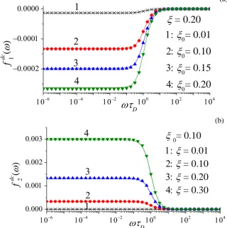
4.6 DC Component of the Dielectric and Kerr-Effect AC Stationary Responses ··· 79

4.7 Generalization to Anomalous Relaxation ··· 81

4.8 Discussion and Conclusion ··· 82

Appendix 4A: Parameters for the Two-Mode Approximation of the Linear Dielectric and Kerr Effect Responses ··· 87

5

DC Response of Uniaxial Magnetic Nanoparticles

···

91

5.1 Exact AC Stationary Solution of DC Magnetization ··· 94

5.2 Limit Values of DC Magnetization ··· 97

5.3 DC Magnetization for  0 ··· 99

5.4 DC Magnetization for  0 ··· 99

5.5 DC Magnetization for Assemblies ··· 109

5.6 Conclusion ··· 111

6

Conclusions

···

113

ix

List of Symbols

A Time-independent five-diagonal system matrix, cf. Eq. (4.17).

( )

A Depopulation factor, cf. Eq. (5.28).

a Diameter of a particle.

, , ,

n n n n

a c d g Coefficients of five-term differential-recurrence relation (2.37).

 Dimensionless damping constant,   M_S.

B Two-diagonal matrix, cf. Eq. (4.17).

 Inverse thermal energy  (kT)1 for electric dipoles, or

inverse thermal energy density  v/ (kT) for magnetic dipoles.

 

n 

C Column vector of F_n_k

 

 in Eq. (2.44) or of k( )

n 

c in Eq. (2.90).

, , , ,

c r a b

C _{ } Clebsch-Gordan coefficients.

 

n t

c Column vectors of Y_{l m,}



 ,

  

t , cf. Eq. (2.82).

( )

k n 

c Column vectors of c_{n m}k_, ( ) , cf. Eq. (2.86).

, ( )

k n m

c  Coefficients of Yn m, ( )t expanded as a Fourier series in time, cf.

Eq. (2.85).

( ) ( )

m t

c Column vectors of f_n m in Eq. (4.16).

n k

c Coefficients of n1

 

t expressed in an infinity of relaxation

modes, cf. Eq. (4.31).

 

nk

  Complex susceptibilities.

( )

HN

  Havriliak-Negami complex susceptibility.

( )

CC

x ( )

CC

  Cole- Davidson complex susceptibility.

( )

D

  Debye complex susceptibility.

0( , 0, )

    DC magnetization of ferrofluid.

nk

 , _nk

 

0 , _S Static susceptibilities, see Section 2.7.

R

D , k Proportionality constant, cf. Eqs. (2.12) and (2.56).

t

D

 Riemann-Liouville fractional derivative, cf. Eq. (2.135).

d Solid angle on the unit sphere, d sin  d d .

nk

 , nk W

 Parameters of the two-mode approximation, cf. Eqs. (2.125)

and (2.126).

,

n m

 Kronecker’s delta, equal to 1 if m=n and to 0 otherwise.

 

t

E External electric field.

 

E z Mittag-Leffler function, cf. Eq. (2.136).

, ,

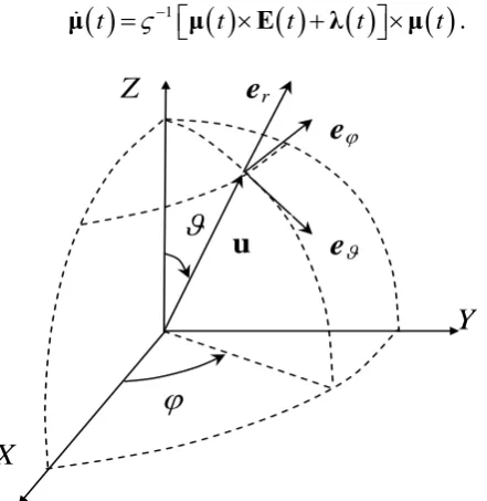
r  

e e e Unit vectors in the direction of r, ,  increasing, see

Fig. 2.1.

, , ,

l m l m

e   Coefficients in the general differential-recurrence

relation (2.73).

erfi( )z Error function of imaginary argument.

 

n

k

F_  Fourier amplitudes of fn

 

t expanded as a Fourier series in

time, cf. Eq. (2.40).

 

_{ }

,

m n k

F  Fourier amplitudes of fn

 

t approximated by a Fourier series

in time via the perturbation approach, e.g., Eq. (4.36).

 

n

f t Statistical moment for ac stationary response in 2D rotational

diffusion model, f_n

 

t  P_n

 

t .

 m n

xi

 1

_{ }

,

n off

f t Linear step-off solution of f_n

 

t , cf. Eq. (2.108).

 

,

l m

f t Time-dependent coefficients of Ψ , ,



  t



expanded in

spherical harmonics, c.f. Eq. (2.60).

( )

n

f  Average of f_n

 

t over a period of the ac field, cf. Eq. (4.70).

 

G t Green function (the unit impulse response) , cf. Eq. (2.111).

 

t

H External magnetic field including ac and dc components.

0

H External dc bias magnetic field.

H External ac magnetic field vector.

h Unit vector in the direction of the magnetic field.

h Dimensionless dc field parameter, h0/ (2 ) .

 Phenomenological damping parameter (viscosity).

I Identity matrix of infinite dimension.

I Moment of inertia of the sphere.

J Probability current, JJ_d J_diff.

d

J Drift current density, J_d Wu.

diff

J Diffusion probability current, Jdiff kuW .

,

J_ J_ Components of J in the coordinate system of e e_r, _,e_.

( )

K t Kerr effect response, cf. Eq. (3.11).

K Anisotropy constant.

k Boltzmann constant.

FP

L Fokker-Planck operator, cf. Eq. (2.57).

2 ˆ _, ˆ ˆ_,

Z

xii

 

t

λ White noise driving torque, cf. Eq. (2.3).

k

 Eigenvalues of L_FP (₁ is the smallest non-vanishing one).

 Ratio of ac and dc field strength, E E/ ₀.

M, M( )t Magnetic dipole moment (function), ~104–105 _B.

S

M Saturation magnetization.

0

M Equilibrium solution for M_( ) , cf. Eq. (5.12).

M_ DC magnetization for assemblies, cf. Eq. (5.30).

( )

M_  DC component of the magnetization m t( ), cf. Eq. (5.11).

( )

H

M t Magnetization of ferrofluid, cf. Eq. (3.32).

( )

m t Stationary solution for the magnetization, cf. Eq. (5.4).

1( )

k

m  Fourier amplitudes of m t( ) expanded as a Fourier series in

time, cf. Eq. (5.9).

0

N Number of particles per unit volume.

μ, μ

 

t Electric dipole moment (function), ~ 0 11 D .

0

 Permeability of free space, 0 4 10 JA m7 2 1

  

 

O Zero matrix of infinite dimension.

( )

P t Electric polarization response, cf. Eq. (3.10).



cos



n

P  Legendre polynomial.

 

,



cos

  

n n

P t P  t Expectation value of Pn



cos



, cf. Eq. (2.34).

(2) 2 ( )

Φ , (3) 1 ( )

Φ Matrices used in Eqs. (4.19) - (4.21).

 

km t

xiii (1)

1 ( )

φ , φ(2)₀ ( ) Column vectors of Eqs. (4.19) - (4.21).

Ψ Wave function in quantum mechanics.

 Angle between the external field and easy axis, see Fig. 5.1.

,

n n



Q Q Matrices of statistical moments in three-term matrix

recurrence relation, e.g., Eq. (2.44)

n

q , q_n, p_n, p_n Supermatrix coefficients of the differential-recurrence

relation (2.81).

, ,

r   Radial, polarand azimuthal angle coordinates of the spherical

polar coordinate system (Fig. 2.1).

IHD i

 Kramers escape rates in the intermediate-to-high damping

(IHD) limit.

 Gyromagnetic ratio.

2 1, , 3

   Direction cosines of h.

( )

n 

S Function rendering C_n

 

 in terms of the next lowest order

one, C_n( ) S_n( ) Q_n( ) C_n1( ) .

i

S Action calculated at the saddle point of the ith well.

 Dimensionless inverse temperature parameter,   K.

 Viscous drag coefficient.

T Absolute temperature.

D

 Debye relaxation (free diffusion) time, D  / 2



kT



.

N

 Free diffusion time of the magnetization, ~ 101110 s8 .

ND

 Free diffusion time of ferrofluid.

eff

n

 Effective relaxation time, cf. Eq. (2.117).

n

 Integral relaxation time, cf. Eq. (2.116).

xiv

u Unit vector along the dipole moment.

, ,

X Y Z

u u u Direction cosines of u.

V Potential energy of electric dipole, or free energy density of

magnetic dipole.

,

V V_{ } Half sided sums of V , Eq. (2.71).

t

V Time-dependent potential.

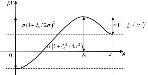
V

 _{Potential barrier,} 2

0

(1 / 2 )

V

    .

,

r s

v Coefficients of the Fourier series expansion of V, cf.

Eq. (2.74).





0 ,

W   Equilibrium Boltzmann distribution.



, ,



W   t Distribution function of 3D rotational diffusion.

 

,

W  t Distribution function of 2D rotational diffusion.

 

t

ω Angular velocity.

1

 , 2 Characteristic frequencies of relaxation modes, cf. Eq. (5.26).

pr

 Precessional frequency.

max

 Frequency of the low-frequency peak in the spectra of the

imaginary part of the susceptibility, see, for example, Fig. 4.2.



 Half-width of the spectra of the real part of the susceptibility,

see Fig. 4.2.

2n

X , t₂ n

X etc. Matrix elements of q_n, q_n, p_n, p_n, cf. Eq. (2.83). ( )

nk

X  Normalized complex susceptibilities , X_nk( )   _nk

 

/ _nk.

,

l m

x , y_{l m,} , etc Static coefficients in the differential-recurrence relation

(2.80).

,

t l m x , ,

t l m

y , etc Dynamic coefficients in the differential-recurrence relation

xv

 

t

 Dimensionless external field parameter.

0

 Dimensionless strength of the external dc electric field

 

0 E0/ kT

  or magnetic field ₀ v₀M H_{S 0}/

 

kT .

 Dimensionless strength of the external ac electric field

 

0 E/ kT

  or magnetic field  v₀M H_S /

 

kT .

1

 Small dimensionless probing applied field strength.

Y, Zn Submatrices of n, n



Q Q , cf. Eq. (2.46).





, ,

l m

Y   Spherical harmonics.

, ( )

n m

Y t , Y_{l m,}

 

t ,



  

, ,

l m

Y   t

Statistical moment, i.e., expectation value of Y_{l m,}



 ,



, cf. Eq. (2.67).

Z Partition function, cf. Eq. (2.101).

 Laplacian on the surface of the unit sphere, cf. Eq. (2.18).

 Gradient on the surface of the unit sphere, cf. Eq. (2.17).

  Divergence on the surface of the unit sphere, cf. Eq. (2.13).

0

1

1

Introduction

When studying the nonlinear effects of polar dielectrics subjected to an ac driving force,

one of the most interesting cases is where a strong ac force and a strong dc bias force are

applied simultaneously. If we compare this situation to a system [1-3] where (a) a strong

ac force is applied alone or (b) a strong dc bias force is applied alongside a weak ac force,

we can observe new effects due to the entanglement of the nonlinear ac and dc responses.

Many of these new effects are of particular interest as they depend on the frequency of the

driving ac field. In this thesis I considered these nonlinear effects on the ac stationary

response in three systems: (i) noninteracting electric/magnetic dipoles; (ii) permanent

electric dipoles in the mean field potential; and (iii) magnetic nanoparticles. The approach

developed is then generalized to treat anomalous relaxation for disordered materials and

complex liquids.

In a dipolar system consisting of an assembly of electrically noninteracting particles

with permanent electric moment μ in a time-varying external electric field E

 

t , the torque due to the external field tends to align the particles in the direction of the applied

field, thus causing the system to become polarized. The polarization P( )t in dielectrics is usually delayed with respect to the time-varying electric field, resulting in dielectric

relaxation which is measured relative to the mean dipole moment in the direction of the

electric field [1],

 

 

~ co

( ) / s

E

P t μ E t E  t , (1.1)

i.e., the expectation value P₁



cos

  

t of the first Legendre polynomial P₁



cos



( being the polar angle of the electric dipole moment vector μ of the molecule). Dielectric

relaxation of electric dipoles in a time-varying electric field is analogous to magnetic

relaxation of magnetic dipoles Μ in a time-varying magnetic field H

 

t , where the mean moment is then in the direction of the magnetic field of M H

 

t /HM_S cos

 

t

[4], i.e., also ~ P₁



cos

  

t . Furthermore, when a dipolar system comprised of polar and anisotropically polarizable particles is acted on by an external electric field E, it

2

birefringence can be described by the electric birefringence function K(t) which is defined using the expectation value of the second Legendre polynomial P₂



cos

  

t as [1]









2 0 0

|| 2

( )~ cos ( )

K t E  _ P  t (1.2)

where _||0 and 0

 are the components of the optical polarizability due to the electric field

(optical frequency) of the light beam passing through the liquid medium. This

electro-optical (Kerr) effect is a purely nonlinear phenomenon. Related nonlinear phenomena

include nonlinear dielectric relaxation of polar liquids and nematic liquid crystals and

nonlinear magnetic relaxation of ferrofluids (colloidal suspension of magnetic

nanoparticles). The theories describing all these nonlinear phenomena, regardless of the

physical system being considered, usually have been based on very similar mathematical

approaches (Langevin equation [1] and/or Fokker-Planck equation [5]) involving the

rotational Brownian motion of a rigid body in an external potential.

The starting point for analysing nonlinear dielectric relaxation and Kerr effect

phenomena in dipolar systems is usually either the Langevin equation or the corresponding

Fokker-Planck equation for the noninertial rotational diffusion model in the mean field

potential when inertial effect are neglected. The Fokker-Planck equation (also called the

Smoluchowski equation), directly derived from the Langevin equation, describes the time

evolution of the orientational distribution function of a particle on a unit sphere. Here, we

shall use the Planck equation approach (see Chapter 2 for details). The

Fokker-Planck equation for the probability distribution function W



 , ,t



of orientations of Brownian particles can be written down in a general form as [1]

2

2 2

2

1 1

sin

sin sin

1 1

sin ,

sin sin

W W W

D t

D V V

W W

kT



    



     

 

 _    _ 

   

 _      _

        

 _{  } _{ }

       

 

(1.3)

where  and  are the polar and azimuthal angles in Fig. 2.1, respectively, V is the mean field potential, D is the rotational diffusion coefficient, k is the Boltzmann constant, and

3

 

,

 

sin

V  t  E t . (1.4)

Equation (1.3) can also be used to evaluate the dielectric response of permanent electric

dipoles in the mean field potential if V is composed of a mean-field potential part and a field dependent part, for example,

 

2

 

o

, c s sin

V  t K E t . (1.5)

Now, the theory of dielectric relaxation of polar fluids bears a close resemblance

to the theory of magnetic relaxation of single domain ferromagnetic particles as

formulated by Brown [6]. Fine single domain ferromagnetic particles possessing internal

magnetocrystalline anisotropy potential, which, by their very nature, have several

equilibrium states with potential barriers between them, exhibit unstable magnetization behaviour due to thermal agitation, causing superparamagnetism and magnetic viscosity. When the barrier energy is comparable to the thermal energy, a change in field will lead

to a change in magnetization due to the large magnetic dipole moment (lagging, however,

behind the field change) analogous to the solid state-like (Arrhenius) Debye relaxation

process in polar dielectric solids over a potential barrier. Brown’s major contribution to

this theory was the derivation of the Fokker-Planck equation for the distribution function

of the particle magnetic moment orientations on the unit sphere:

2

N

2

1 1

sin

2 sin sin

1

sin ,

sin

W W W

t

v V V

W W

k

kT

V T

W V

v

W



    

   



  





 

   

 

 

 

 

 

 _     _ 

   

       

     

 _  _

 

 

 _{ }

 

 

 



 

    

 _{ }

 _    _

(1.6)

where V is now the particle free energy per unit volume, _N is the free diffusion relaxation time,  v/

 

kT , v is the volume of the particle, and  is the damping coefficient. When

   with N const, i.e., ignoring the gyromagnetic term, Brown’s Fokker–Planck

equation (1.6) has the same mathematical form as the noninertial rotational diffusion equation, Eq. (1.3).

To treat the longitudinal relaxation in axially symmetric potentials V

 

,t where the azimuthal angle dependence may be ignored (see, e.g., Eq.(2.19) below), both Eqs. (1.3)

4

solutions may be expanded as a series of Legendre polynomials P_n



cos



(see Eq. (2.23) below). In the general case where the azimuthal angle must also be considered, solutions

of Eqs. (1.3) and (1.6) may be presented as a series of spherical harmonics, Yn m,



 ,



(see e.g., Eqs. (2.59) and (2.60) below). After substituting the general solutions into the

diffusion equations, Eqs. (1.3) and (1.6), the problem is reduced to the solution of an

infinite hierarchy of differential-recurrence relations of the expectation values of the

Legendre polynomials P_n



cos



( )t (or spherical harmonics Y_{n m,}



 ,



( )t ), which can be solved by using the matrix continued fraction method (see Chapter 2 for details).

As we have seen above, the physical quantities of interests describing the ac stationary

response of dielectric and Kerr effect relaxation are the electric polarization function,

1

~P(cos ) ( )  t , and the electric birefringence function, ~P₂(cos ) ( )  t , respectively. To review the previous treatments of the nonlinear dielectric and magnetic relaxation

in dipolar systems, we start with Debye’s theory of dielectric relaxation of polar molecules

using two distinct models of the phenomenon [7]. In the first of the two models, the

rotation of a polar molecule in a liquid composed of noninteracting polar molecules is

treated as a type of Brownian motion [7] (e.g., Eq. (1.4)). This theory can be used to predict

the dispersion and absorption of microwave (GHz) radiation by polar fluids and is the

principle underlying the microwave oven as the dipoles cannot keep in phase with the fast

field. The phase lag results in heating as energy is interchanged with the bath. Put more

precisely, the energy of the dipoles is dissipated via friction due to the bath, which may be

regarded as a collection of harmonic oscillators. Debye also considered a second solid state-like mechanism of relaxation which mainly pertains to relaxation in solids, whereby a dipole can stay either of two directions (i.e., parallel or antiparallel to the applied field)

and reverse its direction by crossing over a potential barrier due to thermal agitation which

is modelled by Brownian motion (e.g., Eq. (1.5)). The relaxation time (the time to cross

the barrier from one orientation to the other) is an Arrhenius process and is thus

exponentially long [8]. This discrete orientation model was used much later by Néel in

order to calculate the relaxation time of the magnetization of fine single-domain

ferromagnetic particles [9]. His calculation is a famous generalization of the Debye theory

to treat the overbarrier relaxation process via the rotational Brownian motion of a rodlike

particle in an external mean field uniaxial potential, commonly called the Maier-Saupe

5

Now, in this liquid state-like Debye model (cf. Eq. (1.4)), when the stimulus due to

the field is much smaller than the thermal energy, the linear ac response term is sufficient

to determine the relaxation process, as demonstrated by Debye [7]. Much later, the Debye

calculation was extended by Coffey and Paranjape [2] to include terms cubic in the applied

field via perturbation theory. In all cases of nonlinear response, no unique response

function exists as it always depends on the precise form of the stimulus, unlike the linear

response. They studied the response to (i) a strong ac field and (ii) a weak ac field combined with a strong dc bias field. The results of the first case have been compared with nonlinear response measurements by De Smet et al. [10] and Jadżyn et al. [11] and agree with these experiments. Additionally, the perturbation calculation for the strong ac

field was verified by Déjardin and Kalmykov [12] by solving the differential-recurrence

relation generated by the rotational Smoluchowski equation [1] using matrix continued

fractions in the frequency domain (see Section 2.3). They also used this method to consider

the strong ac and dc fields case [13]. In the case (ii) of a weak ac field combined with a

strong dc bias field, the ac field was supposed so weak that terms in its square and higher

are omitted. Subsequently, Déjardin et al. [14] extended this perturbation calculation to include the nonlinear ac terms. Similar results may pertain to the magnetization response

under the influence of strong ac and dc bias fields of a blocked ferrofluid composed of a colloidal suspension of single domain ferromagnetic particles. Here, the solid state-like or

Néel [4] magnetization relaxation (cf. the second Debye model) mechanism over the

internal magnetocrystalline anisotropy-Zeeman energy barriers inside the particle due to

magnetic Brownian motion is frozen so that only the liquid state-like Brownian mechanical motion remains. We remark that the nonlinear relaxation effect is easier to

observe experimentally in the ferrofluid because of the large magnetic moment,

4 5

10 ~ 10 _B , of single domain particles compared to that of polar molecules. This behaviour was experimentally detected by Fannin et al. [15] for a strong ac magnetic field. The perturbation method for calculating the nonlinear response of noninteracting

dipoles (e.g., Eq. (1.4)) described above was then generalized by Coffey et al. [3] to include a mean field potential (e.g., Eq. (1.5)). This paper, which considered the response

to an ac field alone, gave analytic formulas for the nonlinear dielectric and Kerr effect

relaxation based on an existing two mode approximation for linear response in the

6

by two modes only [1]. These are the slow over-barrier relaxation (interwell) mode and a set of fast near-degenerate “intrawell” modes, represented as a single high frequency mode. In the combined field case, however, it is difficult to get closed form results due to the

vector-valued coupling between each member of the hierarchy of differential-recurrence

relations. Since the calculation of the dielectric response of polar molecules in a

mean-field potential is analogous to the problem of magnetic relaxation of single domain

ferromagnetic particles from a mathematical point of view, this approach will also be

extended to the superimposed external dc bias and ac fields case for fine single domain

magnetic nanoparticles with uniaxial anisotropy.

As mentioned above, the solution of the Fokker-Planck equation can be reduced

to that of an infinite hierarchy of differential-recurrence equations for the statistical

moments P_n



cos



( )t or Y_{n m,}



 ,



(t). Generally, these differential-recurrence relations comprise three or more terms. The three-term differential-recurrence equation

can be solved in terms of ordinary infinite continued fractions [5], while recurrence

relations with more than three terms should be solved by the matrix continued fraction

method by converting the equations to a three-term matrix recurrence relation [1]. Here,

the scalar continued fraction method is just a special case of the matrix one. Efficient

numerical algorithms for the calculation of the nonlinear ac stationary response of the

magnetization of uniaxial magnetic nanoparticles have been proposed in Refs. [16-18] by assuming that the dc bias and ac driving fields are directed along the easy axis of the particle, so that the matrix continued fraction methods for axially symmetric potentials as discussed above may be applied. However, in this configuration many interesting

nonlinear effects are suppressed because no dynamical coupling between the longitudinal

and transverse precessional modes of motion exists. These mode coupling effects in the

nonlinear ac stationary response can only be modelled for uniaxial particles driven by a strong ac field applied at an angle to the easy axis of the particle so that the axial symmetry is broken by the Zeeman energy [19-22]. Now, building on the axially symmetric solutions

described in Refs. [16-18], an exact nonperturbative method for the determination of the

nonlinear magnetization of magnetic nanoparticles with an arbitrary anisotropy potential and subjected to a strong ac driving field superimposed on a strong dc bias field has

recently been given by Titov et al. [23]. The method is rooted in posing the solution of the averaged magnetic Langevin equation for the statistical moments (which are now the

7

the frequency domain (see also Section 2.6). So far this method has been used to determine

the dynamic susceptibilities (linear, cubic, etc.) and dynamic hysteresis loops in uniaxial

magnetic nanoparticles in Refs. [21, 23].

Many disordered materials such as glass-forming liquids and polymers have very

significant departures from the Debye behaviour resulting in anomalous relaxation [1, 24].

The relaxation processes in such complex systems are characterized by the temporally

nonlocal behaviour arising from the energetic disorder, which produces obstacles or traps,

simultaneously delaying the motion of the particle and producing memory effects [25].

Thus it is also useful to generalize the nonlinear normal relaxation results to anomalous

relaxation via the fractional Fokker-Planck equation [1, 26].

1.1

Layout of the Thesis

This thesis is organized as follows:

In Chapter 2, the general theory of the dielectric and magnetic relaxation is presented.

The derivations of the noninertial Fokker-Planck equation for the rotational Brownian

motion of dipoles are reviewed first. Then, the differential-recurrence relations for the

statistical moments, Pn



cos



( )t or Yn m,



cos



( )t , are derived for both the electric and magnetic cases. The general solutions in the frequency domain of these

differential-recurrence relations are given via the matrix continued fraction method. These continued

fraction solutions can be used for comparisons with our analytic approximate results for

various models considered in the thesis. In addition, the two-mode approximation and

methods of treating anomalous relaxation in dipolar systems are also discussed.

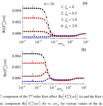
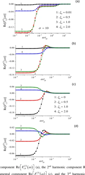
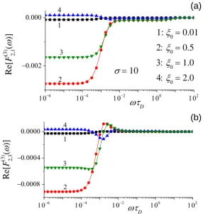
In Chapter 3, the perturbation method is used to calculate the nonlinear ac stationary

response of noninteracting electric and magnetic dipoles for the particular case of a strong

dc bias field superimposed on a strong ac field with a view towards encouraging the

experimental detection of the frequency-dependent dc term, as well as the nonlinear

effects due to the interaction of the two fields at the fundamental and second harmonic

frequencies and the term with the fundamental frequency which also appears in the cubic

response. In particular, we shall highlight the frequency dependence of the dc term and

show the calculation of the dynamic Kerr-effect response as well. We shall also show how

the calculation may be extended to anomalous relaxation governed by a fractional

8

In Chapter 4, the nonlinear dielectric and Kerr-effect relaxation of permanent electric

dipoles, interacting via a mean field potential under the influence of ac and dc bias fields,

are investigated by two complementary approaches. The first is based on perturbation

theory, allowing one to calculate numerically the nonlinear ac stationary responses using

powerful matrix methods, while the second semi-analytic approach, based on the

two-mode approximation [1], effectively generalizes the existing analytic results for dipolar

systems in superimposed ac and dc fields to a mean field potential. The results of this

chapter has been published in Ref. [28].

In Chapter 5, Brown’s continuous diffusion model [6, 29] is applied to investigate the

dc magnetization of uniaxial magnetic nanoparticles in superimposed strong ac and dc

fields. Both cases of an ensemble of fully aligned noninteracting particles and particles

with randomly oriented easy axes are studied using a nonperturbative approach. Here, we

focus for the first time on nonlinear frequency-dependent effects in the dc component of

the magnetization, which were overlooked in previous studies. In the presence of a strong

ac driving field, the dc component of the magnetization of uniaxial particles alters

drastically leading to new nonlinear effects; in particular, it becomes frequency-dependent.

9

2

Diffusion Model of Orientational Relaxation in

Dipolar Systems

In order to study the nonlinear response of dipolar systems in superimposed ac and dc bias

fields, we start by describing how to setup the rotational diffusion model for the electric

and magnetic dipoles where the derivations of the Fokker-Planck equations will be

summarised. Then, the Fokker-Planck equation will be postulated in terms of infinite

hierarchies of differential-recurrence equations for the statistical moments of different

systems which will be solved numerically using the matrix continued fraction method.

Moreover, the basic approximation approaches to yield the analytical formula of nonlinear

responses will be introduced, as well as the equations for the generalization of the results

to the anomalous relaxation.

2.1

Smoluchowski Equation for Electric Dipoles

The Debye theory [7] of dielectric relaxation commences with a special form of the

Fokker-Planck equation for rotational Brownian motion in the space of a sphere when

inertial effects are neglected, which is also called the rotational Smoluchowski equation.

A detailed derivation of this equation is given by Debye [7]. However, we shall follow the

derivation given in Section 1.15 of Ref. [1], which is based on the vector Euler-Langevin

equation of Lewis et al. [31].

To study the rotational Brownian movement of a spherical body, one first assumes

that the homogeneous sphere contains a rigid electric dipole μ [1]. Then the rate of change

of μ

 

t is given by the kinematic relation

 

t 

   

t  t ,

μ ω μ (2.1)

where ω

 

t is the angular velocity of the body and obeys the Euler-Langevin equation

 

 

     

Iω t ω t μ t E t λ t . (2.2)

10





,

( ) 0, ( ) ( ) 2

n t n t m t kT n m t t

          , (2.3)

where the indices n m, 1, 2, 3 in Kronecker’s delta, _{n m,} , correspond to the Cartesian laboratory coordinate axes X, Y, Z. The angular velocity vector after omitting the inertial (I 0) term is

 

1

     

t  _ t  t  t _

ω μ E λ . (2.4)

Substituting Eq. (2.4) into the kinematic relation, Eq. (2.1), we obtain the Langevin equation for the motion of μ in the noninertial limit

 

1

     

 

t  _ t  t  t _ t

μ μ E λ μ . (2.5)

e

_r

e



Y

Z

X

e







[image:27.595.174.395.256.483.2]

u

Fig. 2.1. Spherical polar coordinate system.

Now, the distribution of Brownian particles W

 

μ,t of orientations μ under the influence of an external field E

 

t can be calculated via the continuity equation

div 0

W J , (2.6)

where the current density (flux) JJ_d J_diff contains a conservative part J_d called the drift current density which describes J in the absence of the thermal agitation (i.e. leaving out the term λ

 

t in Eq. (2.5))

d W

J u, (2.7)

where u is a unit vector along the dipole moment μ described by the polarand azimuthal

11

cosines of uare given by uX sincos , uY sinsin, uZ cos. Now, the external field E

 

t  gradV

 

μ,t can be written in the form of

 

1

sin 1

r

V V V

t

u  

   

 _   _

  



  



E e e e , (2.8)

where e_r , e_ and e_ are unit vectors in the direction of increasing r ,  and  respectively. The vector products in Eq. (2.5) are then in spherical coordinates,

1 sin 1

si

1 0 0

n

r

V V

V V V

u

 

 

  

  

 

   

 

  



 

  

e e e

μ E e e (2.9)

and





1 1

sin sin

0 0

0 ,

r

V V V V

 

 



     



 

   

      _  _

  _  _

e e e

μ E μ e e (2.10)

so that the drift current density Jd, Eq. (2.7), is

1 1

sin

d

V V

W

 



  



 _   _

 

 

J e e . (2.11)

Then the diffusion part J_diff of the the current density, which accounts for the thermal agitation, is given by

1 sin

diff R R

W

D D _{ } W

  

  

 

 

     _

 

 

J e e

u , (2.12)

where the diffusion parameter D_Rcan be obtained from the stationary solution of Eq. (2.6) with the Boltzmann distribution W₀



 ,



Z e1 V ,   /kT , where Z is defined by Eq. (2.101). Hence, by substituting Eqs. (2.11) and (2.12) into the divergence of the total

current density J

1 1

div (sin )

sin sin

J

J_ 



   

 

   

 

J J , (2.13)

12 1

1 1 1

, sin , sin R R W D V J V

J W D W

                         (2.14)

Eq. (2.6) yields the rotational Smoluchowski equation for the orientations of μ on a unit

sphere 2 2 1 1 sin sin sin 1 1 sin . s n 2 i D W V V W T W W t k                      _{ } _ _{ } _{ }                  _{  }  _{  }               (2.15)

which can be written in a vector form as





1 (2 _D)

W

W W V

t  



 _{     }

 

 . (2.16)

Here _D / (2kT) is the Debye relaxation time,  (kT)1 is the inverse thermal energy, k is Boltzmann’s constant, T is the absolute temperature, and  and  are the gradient and Laplacian on the surface of the unit sphere, respectively,

1 sin          

 e  e , (2.17)

2

2 2

2 1 1

sin

sin    sin  

      _{ }       

 . (2.18)

Debye [7] specialized this equation to the case where an external field Eis applied along

the polar axis. Here, due to the axial symmetry, the azimuthal angle dependence may be

ignored, so that Eq. (2.15) becomes

1

2 sin

sin

D

W W V

W t         _    _      

      . (2.19)

2.2

Five-Term Differential-Recurrence Relations

The rotational diffusion Smoluchowski equation (2.19) for an axially symmetric problem

can be rewritten as



2





2



2 _D W 1 x W 1 x W V

t x x x x

    _   _  _   _

13

where xcos . The potential V, consisting of the Maier-Saupe uniaxial anisotropy potential and the external field potential of E

 

t applied along the easy axis, can be written as [1]

 

 

2 2

cos cos

V t x t x

        , (2.21)

where   K is a dimensionless inverse temperature parameter, K is the anisotropy constant and 

 

t E t

 

is a dimensionless external field parameter.

By substituting Eq. (2.21) into Eq. (2.20), we have the Fokker-Planck equation for our

specific system,



2





2





 



2 _D W 1 x W 1 x 2 x t W

t x x x

  _  _ _  __  _ _  _ _

      . (2.22)

The general solution of Eq. (2.22) has the form

 

   

0

, _{n n}

n

W t a t P x











, (2.23)

where P zn

 

are the Legendre polynomials [32]. Since the Legendre polynomials form a

complete orthogonal set over



1, 1



, an arbitrary function defined in the interval



1, 1



can be expanded in a series of Legendre polynomials, just like the Fourier series.

Firstly, we consider the term of Eq. (2.22) due to the external field,

 



2



1

t W x

x 

 _{ } _

 . (2.24)

Substituting Eq. (2.23) into this term gives us

 



2





 



2





0

1 n 1 n 2 n

n

t W x a t x P xP

x



 



 _  _  _    _





. (2.25)

Making the use of the recurrence relations of the Legendre polynomials [32],



2







1

1x P_n n P_n xP_n (2.26)

and



 



1 1

1

1

2 1

n n n

xP n P nP

n  

 _   _

 , (2.27)

14

 



2



  

_

_









1 1

0

1 1 2

1 .

2 1 2 1

n n n

n

n n n n

t W x a t P P

x n n

   _{ }         _{  } _{ }      





_{ }   _ (2.28)

The remaining term in Eq. (2.22),



2









2



1 x W 2 x W 1 x

x x x 

  _  _  _{   }

   

     , (2.29)

may be written using Eqs. (2.23) and (2.27) and by making use of the Legendre’s

differential equation [32],



2







1 n 1

n

P

x n n P

x x



  _ _{  }

 

    , (2.30)

so that

















_





_{ }



2 2 2 1 1 0

1 2 1

1

1 2 1 .

2 1

n n n n

n

W

x x W x

x x x

x

a n n P n P nP

x n    _{ }    _  _  _{   }      _  _   _     _{ }  _   _   _{ }  _  _  _{ }  



(2.31)

Substituting Eqs. (2.31) and (2.28) into Eq. (2.22) gives us

  

_

_













_





_{ }



1 1 0 0 2 1 1 0

1 1 2

2

2 1 2 1

1

1 2 1 .

2 1

D n n n n n

n n

n n n n

n

n n n n

a P a t P P

n n

x

a n n P n P nP

x n                       _ _  _         _     _{ }  _   _   _{ }  _  _  _{ }  







(2.32)

Thus, by orthogonality, we have































  



2

2 1 1

2 2

2 2

1

1 2 3 2 1 2 5 2 3

2 1 1 1

.

2 3 2 1 2 3 2 1

D

n n n

n n n

n

a a a

n n n n n n

n

a t a a

n n n n

    _          _{ }   _   _        _  _   _   _ (2.33)

We now rewrite the differential-recurrence relation, Eq. (2.33), in terms of the expectation

values of the Legendre polynomials of order n (statistical moments), viz.,

 

   

1

   

1 ,

n n n

f t P x t W x t P x dx



 

_

, (2.34)

which, using Eq. (2.23) and the orthogonality relation for the Legendre polynomials

 

n

15

   

, 1 1 2 2 1

n m nm

P x P x dx

n 



 



, (2.35)

can be written as

 

 

   

 

 

1 1 , 0 0 2 . 2 1 2 2 1 n m m m n n m n m m

f t a t P x P x dx

a t a t

m n           







(2.36)

Thus Eq. (2.33) becomes

 

 

2

 

2

 

 

1

 

1

 

, Df n t d fn n t g fn n t c fn n t t an fn t fn t

   _  _  _{ }  _ _ (2.37)

where

( 1) , 2(2 1)

( 1)( 1) , (2 1)(2 1)

( 1) 2

1 ,

2 (2 1)(2 3) ( 1)( 2)

. (2 3)(2 1)

n n n n n n a n

n n n

c

n n

n n d

n n

n n n

g n n                 _  _          (2.38)

This five-term differential-recurrence relation (2.37) is used to study the nonlinear

dielectric relaxation and dynamic Kerr effect of permanent dipoles in an axially symmetric

uniaxial mean field potential as shown in Chapter 4. Equation (2.37) can also be used to

consider the nonlinear response of noninteracting electric and magnetic dipoles by setting

0

  , so that Eq. (2.37) reduces to a three-term differential-recurrence relation

  

      

_

_

1

 

1

 

1 1

2 2 2 1

D n n n n

n n n n

f t f t t f t f t

n

     _{ }  _ _

 , (2.39)

which we will use in Chapter 3.

2.3

Calculation of the Stationary Response of Electric Dipoles

via the Matrix Continued Fraction Method

In the current situation the external fields are applied along the easy axis of the particle so

that the problem becomes axially symmetric and the relaxation functions depend only on

16

to the solution of an infinite hierarchy of differential-recurrence equations (2.37) for the

expectation values of the Legendre polynomials P_n



cos



. We remark that the Fokker-Planck equation (2.58) for the uniaxial magnetic nanoparticles under the influence of the

combined fields applied along the easy axis has an identical mathematical form to the

rotational Smoluchowski equation (2.19) used here so that it can be solved using the same

method. The ac stationary solution of the five-term differential-recurrence equation (2.37)

subjected to the combined ac and dc fields has been developed in Refs. [18, 33] which we

will summarize in this section.

The ac stationary solution of Eq. (2.37) may be written as the Fourier series

 

 

ik t n

n k k

f t F  e 









(2.40)

where the Fourier amplitudes satisfy F_n_k 

 

F_kn * (the asterisk denotes the complex conjugate). On substituting Eq. (2.40) and the applied field 

 

t  ₀ cost into Eq. (2.37), we have the set of recurrence relations for the Fourier amplitudes F_kn, viz.,

















2 2

1 1 1 1 1 1

1

0 /2 1 1 1 0,

n D n n

n

n n n

k k k

n n n n n n

k k n k k k k

d ik F c F g F

F F F F F F

a a



 

 

     

   

 

 



 



   (2.41)

where the coefficients a_n, d_n, etc. are given by Eq. (2.38). Now, we introduce a column vector

2 2 1

n n n



 

  

 

c C

c , (2.42)

where the subvector c_n is









2

1

0 0

1

2

0 0

0 0

1 , 0 0 , 0

0 0

0 0

n n n

n

n n

n

F F

n F n

F F  

 

    _{ }

    _{ }

    _{ }

    _{ }

    _{ }

_{ } _{ }   

 

    _{ }

    _{ }

    _{ }

    _{ }

    _{ }

c c c . (2.43)

Now the nine-term scalar recurrence relation (2.41) can be transformed into a three-term