Melbourne at SemEval 2016 Task 11: Classifying Type-level Word
Complexity using Random Forests with Corpus and Word List Features
Julian Brooke Timothy Baldwin
Computing and Info Systems The University of Melbourne
[email protected] [email protected]
Alexandra L. Uitdenbogerd
Computer Science and Info Technology RMIT University
Abstract
SemEval 2016 task 11 involved determining whether words in a sentence were complex or simple for a cohort of people with English as a second language. Training data consisted of 200 annotated sentences, representing the combined judgements of 20 human annota-tors, such that if any annotator of the group labelled a word as complex, then it was con-sidered to be complex. Testing was based on single annotator judgements. Our system used a random forest classifier with a variety of fea-tures, the most important of which were term frequency statistics garnered from four large corpora, and style lexicons built on two large corpora. Minor features in the final system include the presence or absence of words in various readability word lists; many other fea-tures we tried were not successful. Our rank-ing amongst submitted systems did not reflect the strength of our system, due to submitting a far from optimal weighting between complex and simple, but we show that when a more ap-propriate weighting is used, our system ranks amongst the best submitted systems.
1 Introduction
Most work related to readability measurement (Chall and Dale, 1995) focuses on text-level assess-ment, but it is clear that being able to determine the difficulty of individual words is important to both that task as well as related ones such as lexi-cal text simplification (Shardlow, 2014). Although some words can be considered conceptually difficult — that is, a level of intellectual sophistication is re-quired to grasp its meaning — for language learners,
it is more common for words to be considered dif-ficult (or complex) simply because a reader has had little or no exposure to them. This exposure may depend on many different external factors related to the person’s background, some of which may gener-alize across other similar readers, while others may be entirely idiosyncratic to the reader in question. For example, those who study academic English, or operate in an academic environment, have a different vocabulary exposure to those who specialize in hos-pitality English. Therefore, there is value in not only trying to predict some prior difficulty of a word, but also trying to generalize across readers in a similar cohort. Task 11 of the 2016 SemEval competition (Complex Word Identification) is aimed at address-ing this challenge.
This paper describes our system for the task. We commenced with previous work in word readability scoring (Brooke et al., 2012) and stylistic lexicon creation (Brooke and Hirst, 2013; Brooke and Hirst, 2014). For features, we drew on a diverse set of corpus-based and human-derived metrics, and built a random forest-based classifier. While a mistake related to the proper distribution of complex versus simple words prevented us from scoring amongst the top teams in either of the evaluations metrics used in this task, we show that by appropriate class weight-ing with the same classifier and features, we can ob-tain results on either metric that are competitive or better than the best teams.
2 Background
The motivation for SemEval 2016 Task 11 was the need to automatically identify complex
words (Shardlow, 2013) for the task of automated text simplification (Shardlow, 2014). However, the modelling of word complexity and text complex-ity has a long history, much of it using the term readability, and intended for finding reading mate-rial of an appropriate level of difficulty for children and language learners (Chall and Dale, 1995). The measurement of word readability, or lexical com-plexity, is a fundamental component for a range of techniques and their applications beyond automated text simplification: text readability measurement is used as a basis for automatically recommending reading to language learners (Collins-Thompson and Callan, 2004a); lexical complexity measurement can also allow the automatic glossing of reading mate-rial presented electronically (Walmsley, 2011), or the display of text comprising a mixture of two lan-guages (Uitdenbogerd, 2014).
Early work on readability resulted in a large num-ber of measures being developed, typically based on tests given to school-aged native speakers of En-glish (Klare, 1974). The majority of these mea-sures had two recognizable components: grammat-ical difficulty and word difficulty. The word dif-ficulty component of the measures had the follow-ing varieties: inclusion in a list of generally known words, such as the Dale-Chall measure (Chall and Dale, 1995); word length in letters, such as the Au-tomated Readability Index (Senter and Smith, 1967) and Coleman-Liau formulae (Coleman and Liau, 1975); word length in syllables, such as the Flesch and Kincaid formulae (Kincaid et al., 1975); the pro-portion of words exceeding a word length threshold in characters, such as Lix; and proportion of words exceeding a length threshold in syllables, such as the SMOG formula (Klare, 1974). Criticism of these early readability measures included their inability to capture conceptual difficulty (Gordon, 1980), lead-ing the field to be abandoned to some extent un-til the current millennium, in which corpus-based techniques, language models, and classifiers be-came popular, and large-scale corpora bebe-came read-ily available (Collins-Thompson and Callan, 2004b; Franc¸ois, 2009).
For second language learners, it has been ob-served that higher frequency of exposure increases the chance that a word is known, leading to a typi-cal vocabulary knowledge profile in which the
per-centage of known words per 1000 in a ranked list by frequency, monotonically decreases (Meara, 1992). When language learning is optimized based on word frequency, as is often recommended by researchers of language acquisition (Sinclair and Renouf, 1988), the effect may even be exaggerated.
3 Data
The training data released for this task included about 200 sentences, in which each word token that was not a proper noun was annotated as either com-plex or simple. A word was considered comcom-plex if any one annotator from a set of 20 annotators marked it as such. We found many sentences be-ing tagged entirely or almost entirely as complex, for no obvious reason; for training, we excluded any sentence where the number of complex words was greater than or equal to the number of tagged words minus 2, leading to 29 sentences being removed. We also excluded from training any appearances of a set of 140 closed-class function words, which we always classified as simple; both test and training data have words from our list that were tagged as complex, but these appear to be mostly errors, and in general we didn’t want our classifier focusing on classifying extremely common words.
After applying these two filters, the total number of tokens tagged complex in the training set was 427, and the total number of tokens tagged simple was 1234, or roughly a 3 to 1 ratio of simple to complex. By contrast, the test set, which was the result of an-notation by individual annotators of about 9000 sen-tences, had a ratio of simple to complex of almost 18 to 1 (after the common words are removed), which is an extreme difference in class distribution; though we expected to see this effect, when we prepared our system we had no good way of estimating its magnitude. Late in the competition, the organizers released individual annotations which allowed for a more accurate estimate of the expected class distri-bution, but we became aware of that only after the competition was over, and our work here is based on optimizing using the initial class distribution.
4 Lists of Features
Major features are those which we believe are es-sential to the good performance of the model; minor features were helpful in the version of the classifier we used here, based on 20-fold cross-validation in the training set, but the effect was fairly modest; and unused features were not found to be helpful, but we include them for completeness to give a full sense of everything we tried. There are too many features (and too many combinations) to offer up individual numerical analysis of what worked and what didn’t. Our features were selected by optimizing G-score (see Section 6) with a 20-fold cross-validation of the training set.
4.1 Major Features
Term frequency statistics We collected term fre-quency statistics from four large corpora: the British National Corpus (“BNC”: Burnard (2000)), the Gi-gaword corpus (Graff and Cieri, 2003), the In-ternational Conference on Web and Social Me-dia (ICWSM) blog corpus (Burton et al., 2009), and Project Gutenberg (read using the GutenTag tool (Brooke et al., 2015)). We consciously chose corpora that had significant variety with respect to their genre, with the intent of allowing the classifier to focus in on particular kinds of words that certain groups might have trouble with. Note that we typi-cally used the count for the specific word type, but where it didn’t exist in the corpus we substituted the lemma count, rather than giving a count of zero. All of the corpora were of benefit to the final model.
Six style lexicons For the ICWSM and the Project Gutenberg corpora, we built lexicons for six lexical styles using the co-occurrence information in these corpora. The six styles are: literary, abstract, objec-tive, colloquial, concrete, and subjective; each style for each corpus is an individual feature. We used the seed set for the six styles from Brooke et al. (2013), and the co-occurrence profile ranking approach from Brooke and Hirst (2014). We chose these two cor-pora because they are extremely large, varied in con-tent, and we have used and evaluated them in other work; highly constrained language like the newswire text in the Gigaword corpus is unlikely to be of much use for building stylistic lexicons in this fashion.
4.2 Minor Features
Dale-Chall List The presence or absence of the word in the Dale-Chall list, a list of 3000 com-mon words used in the Dale-Chall readability met-ric (Chall and Dale, 1995).
Academic Word List The ranking of the word on the 570-word Academic Word List, which di-vides academic language into 10 frequency cate-gories (Coxhead, 2000).
Beginner List A list of 4636 beginner words, in-cluding words from the Dolch list (Dolch, 1936), previously used as a training/test set in earlier lex-ical readability work (Brooke et al., 2012).
Is Lemma A boolean feature indicating whether a word is its lemma or not. For instance run is a lemma butranis not.
4.3 Unused Features
Document Frequency We tested document quency as a complement or alternative to term fre-quency for the various corpora.
Average Sentence Length The average sentence length of the documents the word appears in, for the 4 corpora used for term frequency. It was a use-ful feature in our earlier work on lexical readabil-ity (Brooke et al., 2012), and is an excellent read-ability feature generally (Uitdenbogerd, 2005).
Word Length The length of the word, in charac-ters, was useful in early iterations but not in the final model.
Average Word Length The average word length in the documents that the word appears in, for the 4 corpora, is another feature from Brooke et al. (2012).
Formality lexicon The formality lexicon built from the ICWSM corpus in Brooke and Hirst (2014). We believe the information in it overlaps considerably with the 6-style lexicon.
Complexity lexicon Using the words from the training set, we attempted to build a complexity dictionary using the method of Brooke and Hirst (2014). The results were not competitive when the six-style lexicon was included.
Latinate affixes A boolean feature which indi-cates the presence or absence of a Latinate affix, which can indicate increased formality (Brooke et al., 2010).
Number of Senses The number of senses of the lemma of the word in WordNet (Fellbaum, 1998).
Hyphen fix For hyphenated words, derive all other statistics using the first word in the hyphenation, in-stead of the whole word.
Bigram style lexicon The features we use do not distinguish between the word type in different con-texts, so we cannot distinguish between word senses. We saw examples of this in the data, such as the word tried in the legal sense inwas tried for mur-der. We made an initial attempt at integrating this information by building a bigram style lexicon, us-ing the same method as the regular method, averag-ing the styles of the two possible contexts, and either replacing the word style or including it as a different feature. However, performance was worse.
Is Cognate While not actually implemented, we considered the possibility of using cognates, which might allow us to discount otherwise complex words which are easy for L2 speakers coming from Eu-ropean language backgrounds because there is a very similar word in other languages (Uitdenbogerd, 2005). However, the results of our early investiga-tion suggested that cognates were not appearing with greater frequency among the simple words than ex-pected, and that therefore the language background of the participants was probably not uniformly Eu-ropean.
5 Classifier
Though rarely competitive on large feature sets, a decision-tree-based classifier has several advan-tages, being considered by some as the only true off-the-shelf classifier (Hastie et al., 2008), in part because it does not require the feature scaling that
is typical in linear classification models, and nat-urally mixes boolean, ordinal and continuous fea-tures without having to convert one to the other. If the number of examples and features is low enough, Random Forests — an ensemble classi-fier that builds multiple decision trees using sub-sets of the examples and features and then combin-ing the individual votes — is a powerful classifier with all the advantages of the basic decision tree (ex-cept interpretability). On the basis of 20-fold cross-validation over the training set, we found that it was the best classifier among a wide range of options (in-cluding all the other ensemble classifiers) that we tested in Sci-kit learn (Pedregosa et al., 2011). We tuned the parameters with an initial feature set, car-ried out feature selection, and then tuned the pa-rameters again, with very little further effect. The only two parameters that were different to the de-fault were the number of estimators (50); and the maximum depth (3). We also tested with different class weights to improve our performance with re-gard to G-score, which is discussed in the next sec-tion. Having class weights penalizes errors for a par-ticular class more, which effectively forces the clas-sifier to guess that class more often, shifting the class distribution.
6 Evaluation Metrics
The evaluation for this task includes 3 basic met-rics (precision, recall, and accuracy) and two com-bined metrics based on them (F-score and G-score). For precision and recall, the positive class isCOM -PLEX, and this is the basis for calculating F-score.
G-score, the primary evaluation metric for this com-petition, is the harmonic mean of precision and accu-racy, putting extra emphasis on recall for theCOM -PLEX class beyond that which is built into the
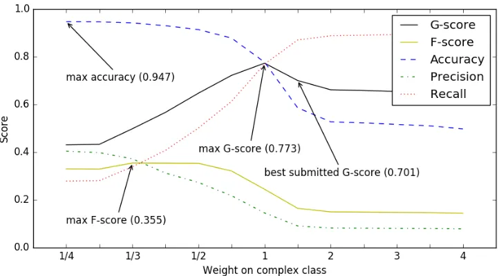
Figure 1:Scores for various metrics for different weightings of theCOMPLEXclass
7 Results
Figure 1 shows the performance of our system for the various metrics across different weightings of the COMPLEX class. With regard to G-score and
F-score, our best submitted system is far from op-timal, since we overestimated the effect of G-score, and underestimated the influence of the class imbal-ance between the training and test sets; we incor-rectly put too much weight on the COMPLEXclass,
which resulted in a G-score of 0.701 (12th ranked) for the 1.5 weighting ofCOMPLEX, and 0.647 (19th
ranked) for the 3.0 weighting of COMPLEX.
How-ever, across all possible weightings, our best G-score (0.773), which is our system without any weighting at all, is tied with the second best G-score in the competition (the best score was 0.774). If we put more weight on simple words, we reach the maxi-mum F-score of 0.355 when the ratio is (roughly) 3 to 1 in favor of simple words; this F-score is better than any other reported F-score (the best F-score of a submitted system is 0.353), though we note that teams might have been more focused on optimizing G-score, since it was the primary metric. Accuracy is maximized simply by minimizing the number of
COMPLEX guesses, and in fact guessing only SIM -PLEwill net an accuracy of 0.953, which is
impossi-ble for our system to beat.
Table 1 shows the results of a small feature
ab-Features G-score F-score
All Features 0.773 0.355 No term frequency 0.550 0.001 No 6-style lexicon 0.748 0.349 No minor features 0.772 0.347
Table 1:Feature ablation
lation study using the best system with regard to each the two combined metrics (no weighting for G-score, 1/3 weighting for F-score); results were er-ratic for less than optimal values. Term frequency information is clearly the most important source of information for deciding complexity, but we also see improvements due to the stylistic lexicons built us-ing co-occurrence information, and the minor fea-tures. The effects are not consistent with respect to degree across the two metrics, likely because differ-ent feature sets result in substantially differdiffer-ent class distributions, which in turn have very different ef-fects on G-score and F-score.
8 Discussion
these systems (or other systems, for that matter) are better. From our perspective, it is unfortunate for us that the organizers created a situation where the class distribution in the test set was very unclear. As it happens, the use of G-score almost exactly counters the effect of the class imbalance (in fact, it seems as if G-score may have been selected ex-actly for this purpose), such that a classifier built on the training data with an eye to F-score will do well with regard to G-score over the testing data (though not the training data), but it didn’t seem obvious to us that this would be the case. More generally, we wonder whether some kind of ROC metric might not be more appropriate for this task. In our opinion, the quality of a model of complexity is orthogonal to producing a class distribution which optimizes a particular metric, and collapsing the two just creates confusion and might lead us to overlook otherwise good approaches.
Most of our performance seems to be due to term frequency and word co-occurrence information from a set of four large corpora. Although using multiple corpora was helpful, we actually rather doubt that our model is learning much that is particular to the group of people involved; more likely it is learning a more general model of word difficulty. Choosing the correct proficiency level is primarily a matter of choosing the best class distribution (via weight-ing); if one has individual annotations of the target population (which we didn’t use, but were eventu-ally made available), this is relatively straightfor-ward. What would have been more interesting is if the task had involved multiple groups with very distinct characteristics (for example, two very differ-ent L1 language backgrounds, or L1 children versus L2 adults), so that a good model would have had to truly adapt to the specific characteristics of different groups to be successful. It would also be interest-ing to see if we could build models that can adapt to individuals, predicting words that a reader would or wouldn’t know based on a small sample of words tagged by them only. Such a setup might bring us closer to the goals that motivate the task.
References
J. Brooke and G. Hirst. 2013. Hybrid models for lex-ical acquisition of correlated styles. In Proceedings
of the 6th International Joint Conference on Natu-ral Language Processing (IJCNLP ’13), pages 82–90, Nagoya, Japan.
J. Brooke and G. Hirst. 2014. Supervised ranking of co-occurrence profiles for acquisition of continuous lexical attributes. In Proceedings of The 25th In-ternational Conference on Computational Linguistics (COLING 2014), pages 2172–2183, Dublin, Ireland. J. Brooke, T. Wang, and G. Hirst. 2010. Automatic
ac-quisition of lexical formality. In Proceedings of the 23rd International Conference on Computational Lin-guistics: Poster Volume (COLING ’10), pages 90–98, Beijing, China.
J. Brooke, V. Tsang, D. Jacob, F. Shein, and G. Hirst. 2012. Building readability lexicons with unanno-tated corpora. InProceedings of the 1st Workshop on Predicting and Improving Text Readability for target reader populations, pages 26–35, Montreal, Canada. J. Brooke, A. Hammond, and G. Hirst. 2015. GutenTag:
An NLP-driven tool for digital humanities research in the Project Gutenberg corpus. InProceedings of the 4nd Workshop on Computational Literature for Liter-ature (CLFL ’15), pages 42–47, Denver, USA. L. Burnard. 2000. User reference guide for British
Na-tional Corpus. Technical report, Oxford University. K. Burton, A. Java, and I. Soboroff. 2009. The ICWSM
2009 Spinn3r Dataset. In Proceedings of the Third Annual Conference on Weblogs and Social Media (ICWSM ’09), San Jose, USA.
J. S. Chall and E. Dale. 1995. Readability revisited: the new Dale-Chall readability formula. Brookline Books, Massachusetts, USA.
M. Coleman and T. L. Liau. 1975. A computer readabil-ity formula designed for machine scoring. Journal of Applied Psychology, 60(2):283.
K. Collins-Thompson and J. Callan. 2004a. Informa-tion retrieval for language tutoring: An overview of the REAP project. InProc. ACM-SIGIR International Conference on Research and Development in Informa-tion Retrieval, Sheffield, UK. Poster.
K. Collins-Thompson and J. Callan. 2004b. A lan-guage modeling approach to predicting reading diffi-culty. InProceedings of the HLT/NAACL 2004 Con-ference, pages 193–200, Boston, USA.
A. Coxhead. 2000. A new academic word list. TESOL quarterly, 34(2):213–238.
E. W. Dolch. 1936. A basic sight vocabulary. The Ele-mentary School Journal, 36(6):456–460.
C. Fellbaum, editor. 1998. WordNet: An Electronic Lex-ical Database. The MIT Press.
and syntactic difficulty of texts for FFL. In Proceed-ings of the EACL Student Research Workshop, pages 19–27, Athens, Greece.
R. M. Gordon. 1980. The readability of unreadable text.
English Journal, pages 60–61, March.
D. Graff and C. Cieri. 2003. English Gigaword. Lin-guistic Data Consortium, Philadelphia, PA.
T. Hastie, R. Tibshirani, and J. Friedman. 2008.The Ele-ments of Statistical Learning: Data Mining, Inference and Prediction. Springer, 2 edition.
J. Peter Kincaid, Robert. P. Fishburne Jr., Richard L. Rogers, and Brad. S. Chissom. 1975. Derivation of new readability formulas for Navy enlisted personnel. Research Branch Report 8-75, Millington, TN: Naval Technical Training, U. S. Naval Air Station, Memphis, USA.
G. R. Klare. 1974. Assessing readability. Reading Re-search Quarterly, X:62–102.
P. Meara. 1992. EFL vocabulary tests. ERIC Clearing-house.
F. Pedregosa, G. Varoquaux, A. Gramfort, V. Michel, B. Thirion, O. Grisel, M. Blondel, P. Prettenhofer, R. Weiss, V. Dubourg, J. Vanderplas, A. Passos, D. Cournapeau, M. Brucher, M. Perrot, and E. Duches-nay. 2011. Scikit-learn: Machine learning in Python.
Journal of Machine Learning Research, 12:2825– 2830.
R. J. Senter and E. A. Smith. 1967. Automated readabil-ity index. Technical report, DTIC Document.
M. Shardlow. 2013. A comparison of techniques to au-tomatically identify complex words. InACL 2013 Stu-dent Research Workshop, pages 103–109, Sofia, Bul-garia.
M. Shardlow. 2014. A survey of automated text simpli-fication.International Journal of Advanced Computer Science and Applications, 4(1).
J. M. Sinclair and A. Renouf. 1988. A lexical syllabus for language taching. In R. Carter and M. McCarthy, editors,Vocabulary and language teaching. Longman, London, UK.
A. L. Uitdenbogerd. 2005. Readability of French as a foreign language and its uses. InAustralasian Docu-ment Computing Symposium, Sydney, Australia. A. L. Uitdenbogerd. 2014. Tools for supporting
lan-guage acquisition via extensive reading. InFirst Work-shop on Natural Language Processing Techniques for Educational Applications (NLP-TEA 1), pages 35–41, Nara, Japan.