Combining Recurrent and Convolutional Neural Networks
for Relation Classification
Ngoc Thang Vu1,2 and Heike Adel1 and Pankaj Gupta3 and Hinrich Sch¨utze1
1Center for Information and Language Processing, LMU Munich
Oettingenstr. 67, 80538 Munich, Germany
2Institute for Natural Language Processing, University of Stuttgart
Pfaffenwaldring 5b, 70569 Stuttgart, Germany
3Siemens Corporate Technology - Knowledge Modeling and Retrieval
Otto-Hahn-Ring 6, 81739 Munich, Germany
[email protected] | [email protected] [email protected] | [email protected]
Abstract
This paper investigates two different neural architectures for the task of relation classi-fication: convolutional neural networks and recurrent neural networks. For both mod-els, we demonstrate the effect of different ar-chitectural choices. We present a new con-text representation for convolutional neural networks for relation classification (extended middle context). Furthermore, we propose connectionist bi-directional recurrent neural networks and introduce ranking loss for their optimization. Finally, we show that combin-ing convolutional and recurrent neural net-works using a simple voting scheme is accu-rate enough to improve results. Our neural models achieve state-of-the-art results on the SemEval 2010 relation classification task.
1 Introduction
Relation classification is the task of assigning sentences with two marked entities to a prede-fined set of relations. The sentence “We poured the <e1>milk</e1> into the<e2>pumpkin mix-ture</e2>.”, for example, expresses the relation
Entity-Destination(e1,e2). While early research mostly focused on support vector ma-chines or maximum entropy classifiers (Rink and Harabagiu, 2010a; Tratz and Hovy, 2010), recent research showed performance improvements by ap-plying neural networks (NNs) (Socher et al., 2012; Zeng et al., 2014; Yu et al., 2014; Nguyen and Gr-ishman, 2015; Dos Santos et al., 2015; Zhang and Wang, 2015) on the benchmark data from SemEval 2010 shared task 8 (Hendrickx et al., 2010) .
This study investigates two different types of NNs: recurrent neural networks (RNNs) and con-volutional neural networks (CNNs) as well as their combination. We make the following contributions: (1) We propose extended middle context, a new context representation for CNNs for relation classi-fication. The extended middle context uses all parts of the sentence (the relation arguments, left of the relation arguments, between the arguments, right of the arguments) and pays special attention to the mid-dle part.
(2) We presentconnectionist bi-directional RNN modelswhich are especially suited for sentence clas-sification tasks since they combine all intermediate hidden layers for their final decision. Furthermore, the ranking loss function is introduced for the RNN model optimization which has not been investigated in the literature for relation classification before.
(3) Finally, we combine CNNs and RNNs using a simple voting scheme and achieve new state-of-the-art results on the SemEval 2010 benchmark dataset.
2 Related Work
In 2010, manually annotated data for relation clas-sification was released in the context of a SemEval shared task (Hendrickx et al., 2010). Shared task participants used, i.a., support vector machines or maximum entropy classifiers (Rink and Harabagiu, 2010a; Tratz and Hovy, 2010). Recently, their re-sults on this data set were outperformed by applying NNs (Socher et al., 2012; Zeng et al., 2014; Yu et al., 2014; Nguyen and Grishman, 2015; Dos Santos et al., 2015).
Zeng et al. (2014) built a CNN based only on the context between the relation arguments and ex-tended it with several lexical features. Kim (2014) and others used convolutional filters of different sizes for CNNs. Nguyen and Grishman (2015) ap-plied this to relation classification and obtained im-provements over single filter sizes. Dos Santos et al. (2015) replaced the softmax layer of the CNN with a ranking layer. They showed improvements and pub-lished the best result so far on the SemEval dataset, to our knowledge.
Socher et al. (2012) used another NN architecture for relation classification: recursive neural networks that built recursive sentence representations based on syntactic parsing. In contrast, Zhang and Wang (2015) investigated a temporal structured RNN with only words as input. They used a bi-directional model with a pooling layer on top.
3 Convolutional Neural Networks (CNN)
CNNs perform a discrete convolution on an input matrix with a set of different filters. For NLP tasks, the input matrix represents a sentence: Each column of the matrix stores the word embedding of the cor-responding word. By applying a filter with a width of, e.g., three columns, three neighboring words (tri-gram) are convolved. Afterwards, the results of the convolution are pooled. Following Collobert et al. (2011), we perform max-pooling which extracts the maximum value for each filter and, thus, the most informative n-gram for the following steps. Finally, the resulting values are concatenated and used for classifying the relation expressed in the sentence.
3.1 Input: Extended Middle Context
One of our contributions is a new input representa-tion especially designed for relarepresenta-tion classificarepresenta-tion. The contexts are split into three disjoint regions based on the two relation arguments: the left con-text, the middle context and the right context. Since in most cases the middle context contains the most relevant information for the relation, we want to fo-cus on it but not ignore the other regions completely. Hence, we propose to use two contexts: (1) a com-bination of the left context, the left entity and the middle context; and (2) a combination of the mid-dle context, the right entity and the right context.
Due to the repetition of the middle context, we force the network to pay special attention to it. The two contexts are processed by two independent convo-lutional and max-pooling layers. After pooling, the results are concatenated to form the sentence repre-sentation. Figure 1 depicts this procedure. It shows an examplary sentence: “He had chest pain and
<e1>headaches</e1> from <e2>mold</e2> in the bedroom.” If we only considered the middle context “from”, the network might be tempted to predict a relation likeEntity-Origin(e1,e2). However, by also taking the left and right con-text into account, the model can detect the relation
Cause-Effect(e2,e1). While this could also be achieved by integrating the whole context into the model, using the whole context can have disadvan-tages for longer sentences: The max pooling step can easily choose a value from a part of the sentence which is far away from the mention of the relation. With splitting the context into two parts, we reduce this danger. Repeating the middle context increases the chance for the max pooling step to pick a value from the middle context.
3.2 Convolutional Layer
Following previous work (e.g., (Nguyen and Grish-man, 2015), (Dos Santos et al., 2015)), we use 2D filters spanning all embedding dimensions. After convolution, a max pooling operation is applied that stores only the highest activation of each filter. We apply filters with different window sizes 2-5 (multi-windows) as in (Nguyen and Grishman, 2015), i.e. spanning a different number of input words.
4 Recurrent Neural Networks (RNN)
He had chest pains and <e1>headaches</e1> from <e2>mold</e2> in the bedrooms. ... ... convolution convolution pooling pooling sentence representation concatenation
Figure 1:CNN with extended contexts
avoid exploding gradients, we use gradient clipping with a threshold of 10 (Pascanu et al., 2012).
4.1 Input of the RNNs
Initial experiments showed that using trigrams as in-put instead of single words led to superior results. Hence, at timesteptwe do not only give wordwtto
the model but the trigramwt−1wtwt+1 by
concate-nating the corresponding word embeddings.
4.2 Connectionist Bi-directional RNNs
Especially for relation classification, the process-ing of the relation arguments might be easier with knowledge of the succeeding words. Therefore in bi-directional RNNs, not only a history vector of word wt is regarded but also a future vector. This
leads to the following conditioned probability for the historyhtat time stept∈[1, n]:
hft =f(Uf·wt+V ·hft−1) (1)
hbt =f(Ub·wn−t+1+B·hbt+1) (2)
ht=f(hbt +hft+H·ht−1) (3)
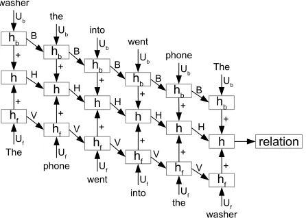
Thus, the network can be split into three parts: a forward pass which processes the original sen-tence word by word (Equation 1); a backward pass which processes the reversed sentence word by word (Equation 2); and a combination of both (Equation 3). All three parts are trained jointly. This is also depicted in Figure 2.
Combining forward and backward pass by adding their hidden layer is similar to (Zhang and Wang, 2015). We, however, also add a connection to the previous combined hidden layer with weight H to be able to include all intermediate hidden layers into the final decision of the network (see Equation 3). We call this “connectionist bi-directional RNN”.
hb hb hb relation hb hb washer the into went phone The hb hf The hf hf
phone hf
into
went hf
the hf washer h h h h h h + + + + + + + + + + + + H H H H H B B B B B V V V V V Ub Uf Ub Ub Ub Ub Ub Uf Uf Uf Uf Uf
Figure 2:Connectionist bi-directional RNN
In our experiments, we compare this RNN with uni-directional RNNs and bi-directional RNNs with-out additional hidden layer connections.
5 Model Training 5.1 Word Representations
Words are represented by concatenated vectors: a word embedding and a position feature vector.
Pretrained word embeddings. In this study, we used the word2vec toolkit to train embeddings on an English Wikipedia from May 2014. We only con-sidered words appearing more than 100 times and added a special PADDING token for convolution. This results in an embedding training text of about 485,000 terms and6.7·109 tokens. During model
training, the embeddings are updated.
Position features. We incorporate randomly ini-tialized position embeddings similar to Zeng et al. (2014), Nguyen and Grishman (2015) and Dos San-tos et al. (2015). In our RNN experiments, we in-vestigate different possibilities of integrating posi-tion informaposi-tion: posiposi-tion embeddings, posiposi-tion em-beddings with entity presence flags (flags indicating whether the current word is one of the relation argu-ments), and position indicators (Zhang and Wang, 2015).
5.2 Objective Function: Ranking Loss
Ranking.We applied the ranking loss function pro-posed in Dos Santos et al. (2015) to train our models. It maximizes the distance between the true labely+
[image:3.612.317.540.63.222.2]x. The objective function is
L= log(1 + exp(γ(m+−sθ(x)y+)))
+ log(1 + exp(γ(m−+s
θ(x)c−))) (4)
with sθ(x)y+ andsθ(x)c− being the scores for the
classes y+ and c− respectively. The parameter γ controls the penalization of the prediction errors and
m+ andm−are margins for the correct and incor-rect classes. Following Dos Santos et al. (2015), we setγ = 2, m+ = 2.5, m− = 0.5. We do not learn a pattern for the classOtherbut increase its differ-ence to the best competitive label by using only the second summand in Equation 4 during training.
6 Experiments and Results
We used the relation classification dataset of the SemEval 2010 task 8 (Hendrickx et al., 2010). It consists of sentences which have been manually la-beled with 19 relations (9 directed relations and one artificial classOther). 8,000 sentences have been distributed as training set and 2,717 sentences served as test set. For evaluation, we applied the official scoring script and report the macro F1 score which also served as the official result of the shared task.
RNN and CNN models were implemented with theano (Bergstra et al., 2010; Bastien et al., 2012). For all our models, we use L2 regularization with a weight of 0.0001. For CNN training, we use mini batches of 25 training examples while we perform stochastic gradient descent for the RNN. The ini-tial learning rates are 0.2 for the CNN and 0.01 for the RNN. We train the models for 10 (CNN) and 50 (RNN) epochs without early stopping. As ac-tivation function, we apply tanh for the CNN and capped ReLU for the RNN. For tuning the hyperpa-rameters, we split the training data into two parts: 6.5k (training) and 1.5k (development) sentences. We also tuned the learning rate schedule on dev.
Beside of training single models, we also report ensemble results for which we combined the pre-sented single models with a voting process.
6.1 Performance of CNNs
As a baseline system, we implemented a CNN sim-ilar to the one described by Zeng et al. (2014). It consists of a standard convolutional layer with filters with only one window size, followed by a softmax
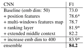
CNN F1
Baseline (emb dim: 50) 73.0 + position features 78.6* + multi-windows features map 78.7 + ranking layer 81.9* + extended middle context 82.2 + increase emb dim to 400 83.9*
[image:4.612.341.513.57.156.2]ensemble 84.2
Table 1: F1 score of CNN and its components, * indicates statisticial significance compared to the result in the line above (z-test,p <0.05)
layer. As input it uses the middle context. In con-trast to Zeng et al. (2014), our CNN does not have an additional fully connected hidden layer. Therefore, we increased the number of convolutional filters to 1200 to keep the number of parameters comparable. With this, we obtain a baseline result of 73.0. After including 5 dimensional position features, the per-formance was improved to 78.6 (comparable to 78.9 as reported by Zeng et al. (2014) without linguistic features).
In the next step, we investigate how this result changes if we successively add further features to our CNN: multi-windows for convolution (window sizes: 2,3,4,5 and 300 feature maps each), ranking layer instead of softmax and our proposed extended middle context. Table 1 shows the results. Note that all numbers are produced by CNNs with a compa-rable number of parameters. We also report F1 for increasing the word embedding dimensionality from 50 to 400. The position embedding dimensionality is 5 in combination with 50 dimensional word em-beddings and 35 with 400 dimensional word embed-dings. Our results show that especially the ranking layer and the embedding size have an important im-pact on the performance.
6.2 Performance of RNNs
RNN F1 uni-directional (Baseline, emb dim: 50) 61.2 uni-directional + position embs 68.3* uni-directional + position embs + entity flag 73.1* uni-directional + position indicators 73.4 bi-directional + position indicators 74.2* connectionist-bi-directional+position indicators 78.4* + ranking layer 81.4* + increase emb dim to 400 82.5*
[image:5.612.331.520.58.194.2]ensemble 83.4
Table 2: F1 score of RNN and its components, * indicates statisticial significance compared to the result in the line above (z-test,p <0.05)
position indicators (Zhang and Wang, 2015)). The results indicate that position indicators (i.e. artificial words that indicate the entity presence) perform the best on the SemEval data. We achieve an F1 score of 73.4 with them. However, the difference to using position embeddings with entity flags is not statisti-cally significant.
Similar to our CNN experiments, we successively vary the RNN models by using bi-directionality, by adding connections between the hidden layers (“connectionist”), by applying ranking instead of softmax to predict the relation and by increasing the word embedding dimension to 400.
The results in Table 2 show that all of these vari-ations lead to statistically significant improvements. Especially the additional hidden layer connections and the integration of the ranking layer have a large impact on the performance.
6.3 Combination of CNNs and RNNs
Finally, we combine our CNN and RNN models us-ing a votus-ing process. For each sentence in the test set, we apply several CNN and RNN models pre-sented in Tables 1 and 2 and predict the class with the most votes. In case of a tie, we pick one of the most frequent classes randomly. The combination achieves an F1 score of 84.9 which is better than the performance of the two NN types alone. It, thus, confirms our assumption that the networks provide complementary information: while the RNN com-putes a weighted combination of all words in the sentence, the CNN extracts the most informative n-grams for the relation and only considers their re-sulting activations.
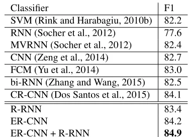
Classifier F1
SVM (Rink and Harabagiu, 2010b) 82.2 RNN (Socher et al., 2012) 77.6 MVRNN (Socher et al., 2012) 82.4 CNN (Zeng et al., 2014) 82.7 FCM (Yu et al., 2014) 83.0 bi-RNN (Zhang and Wang, 2015) 82.5 CR-CNN (Dos Santos et al., 2015) 84.1
R-RNN 83.4
ER-CNN 84.2
ER-CNN + R-RNN 84.9 Table 3:State-of-the-art results for relation classification
6.4 Comparison with State of the Art
Table 3 shows the results of our models ER-CNN (extended ranking ER-CNN) and R-RNN (ranking RNN) in the context of other state-of-the-art models. Our proposed models obtain state-of-the-art results on the SemEval 2010 task 8 data set without making use of any linguistic features.
7 Conclusion
In this paper, we investigated different features and architectural choices for convolutional and recurrent neural networks for relation classification without using any linguistic features. For convolutional neu-ral networks, we presented a new context represen-tation for relation classification. Furthermore, we introduced connectionist recurrent neural networks for sentence classification tasks and performed the first experiments with ranking recurrent neural net-works. Finally, we showed that even a simple com-bination of convolutional and recurrent neural net-works improved results. With our neural models, we achieved new state-of-the-art results on the SemEval 2010 task 8 benchmark data.
Acknowledgments
Heike Adel is a recipient of the Google European Doctoral Fellowship in Natural Language Process-ing and this research is supported by this fellowship. This research was also supported by Deutsche Forschungsgemeinschaft: grant SCHU 2246/4-2.
References
[image:5.612.73.306.60.183.2]Berg-eron, Nicolas Bouchard, and Yoshua Bengio. 2012. Theano: new features and speed improvements. Deep Learning and Unsupervised Feature Learning NIPS 2012 Workshop.
James Bergstra, Olivier Breuleux, Fr´ed´eric Bastien, Pas-cal Lamblin, Razvan Pascanu, Guillaume Desjardins, Joseph Turian, David Warde-Farley, and Yoshua Ben-gio. 2010. Theano: a CPU and GPU math expression compiler. InProceedings of the Python for Scientific Computing Conference (SciPy).
Ronan Collobert, Jason Weston, L´eon Bottou, Michael Karlen, Koray Kavukcuoglu, and Pavel Kuksa. 2011. Natural language processing (almost) from scratch.
The Journal of Machine Learning Research, 12:2493– 2537.
C´ıcero Nogueira Dos Santos, Bing Xiang, and Bowen Zhou. 2015. Classifying relations by ranking with convolutional neural networks. In Proceedings of ACL. Association for Computational Linguistics. Iris Hendrickx, Su Nam Kim, Zornitsa Kozareva, Preslav
Nakov, Diarmuid ´O S´eaghdha, Sebastian Pad´o, Marco Pennacchiotti, Lorenza Romano, and Stan Szpakow-icz. 2010. Semeval-2010 task 8: Multi-way classifi-cation of semantic relations between pairs of nominals. InProceedings of the Workshop on SemEval. Associa-tion for ComputaAssocia-tional Linguistics.
Yoon Kim. 2014. Convolutional neural networks for sen-tence classification. InProceedings of EMNLP. Asso-ciation for Computational Linguistics.
Thien Huu Nguyen and Ralph Grishman. 2015. Rela-tion extracRela-tion: Perspective from convoluRela-tional neural networks. InProceedings of the NAACL Workshop on Vector Space Modeling for NLP. Association for Com-putational Linguistics.
Razvan Pascanu, Tomas Mikolov, and Yoshua Bengio. 2012. Understanding the exploding gradient problem.
Computing Research Repository.
Bryan Rink and Sanda Harabagiu. 2010a. Utd: Classi-fying semantic relations by combining lexical and se-mantic resources. InProceedings of the Workshop on SemEval. Association for Computational Linguistics. Bryan Rink and Sanda Harabagiu. 2010b. Utd:
Classi-fying semantic relations by combining lexical and se-mantic resources. InProceedings of the Workshop on SemEval, pages 256–259. Association for Computa-tional Linguistics.
Richard Socher, Brody Huval, Christopher D Manning, and Andrew Y Ng. 2012. Semantic compositionality through recursive matrix-vector spaces. In Proceed-ings of EMNLP / CoNLL. Association for Computa-tional Linguistics.
Stephen Tratz and Eduard Hovy. 2010. Isi: automatic classification of relations between nominals using a
maximum entropy classifier. In Proceedings of the Workshop on SemEval. Association for Computational Linguistics.
Paul J Werbos. 1990. Backpropagation through time: what it does and how to do it. Proceedings of the IEEE.
Mo Yu, Matthew Gormley, and Mark Dredze. 2014. Factor-based compositional embedding models. In
Proceedings of the NIPS Workshop on Learning Se-mantics.
Daojian Zeng, Kang Liu, Siwei Lai, Guangyou Zhou, and Jun Zhao. 2014. Relation classification via convolu-tional deep neural network. InProceedings of COL-ING.