Textual Aggression Detection through Deep Learning

Proceedings of the First Workshop on Trolling, Aggression and Cyberbullying, pages 177–187

177

Textual Aggression Detection through Deep Learning

Antonela Tommasel∗

ISISTAN UNICEN - CONICET

Tandil, Buenos Aires Argentina

Juan Manuel Rodriguez

ISISTAN UNICEN - CONICET

Tandil, Buenos Aires Argentina

Daniela Godoy

ISISTAN UNICEN - CONICET

Tandil, Buenos Aires Argentina

Abstract

Cyberbullying and cyberaggression are serious and widespread issues increasingly affecting In-ternet users. With the widespread of social media networks, bullying, once limited to particular places, can now occur anytime and anywhere. Cyberaggression refers to aggressive online be-haviour that aims at harming other individuals, and involves rude, insulting, offensive, teasing or demoralising comments through online social media. Considering the dangerous consequences that cyberaggression has on its victims and its rapid spread amongst internet users (specially kids and teens), it is crucial to understand how cyberbullying occurs to prevent it from escalating. Given the massive information overload on the Web, there is an imperious need to develop in-telligent techniques to automatically detect harmful content, which would allow the large-scale social media monitoring and early detection of undesired situations. This paper presents the Isistanitos’s approach for detecting aggressive content in multiple social media sites. The ap-proach is based on combining Support Vector Machines and Recurrent Neural Network models for analysing a wide-range of character, word, word embeddings, sentiment and irony features. Results confirmed the difficulty of the task (particularly for detecting covert aggressions), show-ing the limitations of traditionally used features.

1 Introduction

In recent years, social networking and micro-blogging sites have seen their popularity increased, at-tracting an increasing number of users, who share their personal information and interact with others. Additionally, social media sites allow users to publish content or photos and to comment or tag content published by other users. As social media usage grows, other undesirable phenomena and behaviours appear. Even when most of the time, Internet use is safe, online communications through social media involve risks. In this context, users might have to deal with threatening situations like cyberaggression or cyberbullying, amongst other undesirable phenomena (Whittaker and Kowalski, 2015).

With the widespread of social media networks, bullying, once limited to particular places or times of the day (e.g. schools), can now occur anytime and anywhere (Chatzakou et al., 2017). Cyberaggres-sion refers to aggressive online behaviour that aims at harming other individuals (Hosseinmardi et al., 2015), and involves rude, insulting, offensive, teasing or demoralising comments through online social media (Chavan and S S, 2015). Aggressions could target educational qualifications, gender, family or personal habits, amongst other possibilities.

Given the dangerous consequences that cyberaggression has on its victims, and its rapid spread amongst internet users (specially kids and teens), it is crucial to understand how it occurs to prevent it from escalating. This has important applications on the detection of cyberextremism, cybercrime and cy-berhate propaganda (Agarwal and Sureka, 2015). Nonetheless, several challenges hinder the successful detection of abusive behaviour (Chatzakou et al., 2017; Nobata et al., 2016). First, the lack of grammar correctness and syntactic structure of social media posts hinders the usage of natural language process-ing tools. Second, the limited context provided by each individual post, causprocess-ing that an individual post

∗

[email protected]

might be deemed as normal text, whilst the same post inserted into a series of consecutive posts might be deemed as aggressive. Third, the fact that aggression could occur in multiple forms, besides the obvious abusive language, for example it could be disguised as irony and sarcasm. Fourth, it is difficult to track all racial and minority insults, which might be unacceptable to one group, but acceptable to another one. This article reports the solution proposed byIsistanitosto the shared task of aggression detection (Ku-mar et al., 2018a). To that end, several combinations of feature sets and algorithms were evaluated. The remainder of this article is organised as follows. Section 2 describes related work regarding the detec-tion of both aggressive content and bullying accounts. Secdetec-tion 3 describes the dataset used, the selected features and the proposed model for detecting aggressive content in social media. Section 4 analyses the obtained results. Finally, Section 5 presents the conclusions derived from the study, and outlines future lines of research.

2 Related Work

Research into cyberaggression detection has increased in recent years due to its proliferation across so-cial media, and its detrimental effect on people (Salawu et al., 2017). Cyberaggression or cyberbullying detection can comprise four different tasks (Salawu et al., 2017): identification of the individual aggres-sive messages in a social media data stream, assessment of the severity of the aggression, identification of the roles of the involved individuals, and the classification of events that occur as a consequence of an aggression incident.

Nobata et al. (2016) aimed at detecting hate speech on 2 million online comments from Yahoo! Fi-nance and News. Four types of features were considered: n-grams, linguistic, syntactic, and embed-ded semantic features. Comments were pre-processed by normalising numbers, replacing unknown words with the same token, replacing repeated punctuation. Results showed that combining all features achieved the best F-Measure results. Similarly, Chavan and S S (2015) aimed at distinguishing between bullying and non-bullying comments. The selected features included TF-IDF weighted n-grams, the presence of pronouns and skip-grams. Only the 3,000 highest ranked features according toχ2 were se-lected. Experimental evaluation was based on approximately 6.5k comments from an unspecified site. Posts were pre-processed by removing non-words characters, hyphens and punctuation. Additionally, a spell-checker was applied to correct potential spelling mistakes. Results showed that the best perfor-mance was achieved when considering pronouns and skip-grams.

Unlike the binary classification studied in (Nobata et al., 2016; Chavan and S S, 2015), Van Hee et al. (2015) explored the fine-grained classification of cyberbullying events into 7 categories (non-aggressive, threat/blackmail, insult, curse, defamation, sexual talk, defence and encouragement to the harasser). The authors considered two types of lexical features: bag-of-words features (including unigrams, bigrams and character trigrams) and polarity features (including the number of positive, negative and neutral lexicon words averaged over text length, and the overall post polarity). The evaluation showed a high discrepancy of results amongst the diverse classes, which was allegedly due to the extent to which posts in each category are lexicalised.

In summary, most works have been based on content, sentiment, user, network-based features or a combination of them. Content-based features include the extractable lexical items of documents (e.g. aggressive or hate words), such as keywords, profanity, pronouns, part-of-speech tagging and punctuation symbols. Sentiment features refer to certain keywords, phrases or symbols that indicate the sentiment of emotion polarity of the content. User-based features represent those characteristics on users’ profiles that can be used to judge the role played by such user in a series of online communications (e.g. age, gender or sexual orientation). Finally, network-based features refer to metrics that can be extracted from the social networks (e.g. the number of friends, number of followers, frequency of posting and how many times posts were shared).

3 Methodology and Data

dataset used (Section 3.1), the features selected for characterising aggressive content (Section 3.2) and the predictive model defined (Section 3.3).

3.1 Dataset

The used dataset was presented in (Kumar et al., 2018b). The original version comprised both Hindi and English posts related to pages and hashtags that are commonly discussed amongst Indians inFacebook andTwitter. Particularly, more than 40 Facebook pages were analysed. Selected pages include news sites, Web-based forums, political parties, student groups, and support and opposition groups revolving Indian University current events. In the case ofTwitter, several popular hashtags amongst Indians were selected, including Indian vs. Pakistan cricket matches, election results, and beef ban. Since posts were not curated during the recollection, the dataset includes posts in English, Hindi, and other Indian languages, as well as mixed-language posts. Post were manually tagged into one of three aggression levels:

Overt Aggressive (OAG) comprises posts in which the aggression is clearly expressed by certain

lexical features or syntactic structures that can be always considered aggressive.

Covert Aggressive (CAG)comprises posts in which the aggression is observed by the intent, but not

by their lexical or syntactic structure. Posts in this category might present common polite expressions used in an insincere manner (e.g. irony or sarcasm).

Non Aggressive (NAG)comprises posts that convey no aggression at all. This category also includes

posts written in languages different than English and Hindi.

For the purpose of the Shared Task, the proposed approach was designed only for English posts. The shared task organisers provided both training and validation English sets. Nonetheless, both sets also included several posts written in other languages, which made even more difficult the already challenging task of automatically detecting aggression.

3.2 Features for Characterising Aggression

Aggression is characterised by considering four different sets of features. The first feature set (referenced asGloVe features) describes each post as a sequence of vectors, where each vector represents a word within the modelled post. The vector representation of words is built using GloVe (Pennington et al., 2014)1, a log-bilineal model with a least-squares objective that aims at estimating the probability of a word given its context. The model was trained using the social media dataset presented in (Zubiaga et al., 2015). Vector dimensionality was set to 300as such value was reported to achieve high quality results (Mikolov et al., 2013; Pennington et al., 2014). According to the average post length in the training set, each post was represented by23vectors. For those posts having less than 23 words, vectors were added. Those words that are not defined in the GloVe model are also represented as zero-vectors.

The second feature set (referenced as Sentimentfeatures) also describes each post as a sequence of vectors, where each vector represents the sentiments conveyed by a word according to the SentiWordNet corpus (Baccianella et al., 2010). In this regard, SentiWordNet defines three sentiment scores for synsets inWordNet, namely positivity, negativity, and objectivity. Considering that a particular word might have associated severalWordNetsynsets, its associated vector will contain the average and standard deviation of each score, i.e., the vector will be constituted as(P osavg, N egavg, Objavg, P osstd, N egstd, Objstd). The number of vectors representing a post was set to the average number of words that were associated to aWordNetsynset, i.e.10. The same strategies as for theGloVefeatures were adopted for dealing with shorter post and words without associated synsets.

The third feature set (referenced asComposed features) represents posts as a concatenation of a TF-IDF model, a sentiment analysis model, and several punctuation related features. First, the TF-TF-IDF model is built considering the stems of the words in the training dataset, obtained by means of the Porter Stemmer (Porter, 1980). Then, the TF-IDF models are normalized using L-2 norm. The sentiment analysis model includes four features describing the force of negative, positive and neutral sentiments,

Post Id Text Tokens

2018626 Puppies are way more important

’pup’, ’upp’, ’ppi’, ’pie’, ’ies’, ’es ’, ’s a’, ’ ar’, ’are’, ’re ’, ’e w’, ’ wa’, ’way’, ’ay ’, ’y m’, ’ mo’, ’mor’, ’ore’, ’re ’, ’e i’, ’ im’, ’imp’, ’mpo’, ’por’, ’ort’, ’rta’, ’tan’, ’pupp’, ’uppi’, ’ppie’, ’pies’, ’ies ’, ’es a’, ’s ar’, ’ are’, ’are ’, ’re w’, ’e wa’, ’ way’, ’way ’, ’ay m’, ’y mo’, ’ mor’, ’more’, ’ore ’, ’re i’, ’e im’, ’ imp’, ’impo’, ’mpor’, ’port’, ’orta’, ’rtan’, ’puppi’, ’uppie’, ’ppies’, ’pies ’, ’ies a’, ’es ar’, ’s are’, ’ are ’, ’are w’, ’re wa’, ’e way’, ’ way ’, ’way m’, ’ay mo’, ’y mor’, ’ more’, ’more ’, ’ore i’, ’re im’, ’e imp’, ’ impo’,

’impor’, ’mport’, ’porta’, ’ortan’, ’puppi’, ’are’, ’way’, ’more’, ’import’

Table 1: N-gram TF-IDF features

and a composed score. These scores are obtained according to the Vader model (Hutto and Gilbert, 2014), which reported a F-Measure of 0.96 on Twitter. Additional features are added to account for the negative, positive and neutral sentiment score conveyed by emojis, according to (Kralj Novak et al., 2015). Interestingly, only5.75%of the training posts had emojis, hence in case posts do not have any emoji, features are set to zero. Finally, punctuation related features analyse whether posts have two consecutive dots or commas, question marks, admiration marks, non-printable characters (such as emojis or non-latin characters), and quote marks (“”).

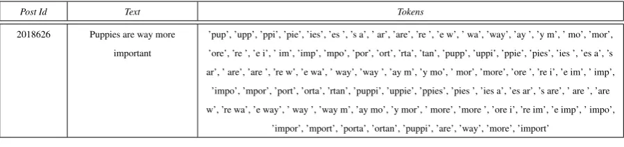
Finally, the fourth feature set (referenced asN-gram TF-IDFfeatures) represents posts as a normalised TF-IDF model that considers not only the word stems, but also all the possible 3-grams, 4-grams, and 5-grams within the post. Adding n-grams to the word stems aims at capturing different misspellings of words, which are fairly common within the considered dataset. Table 1 presents an example of the tokenisation used for this feature set, in which the last five tokens are stems of the post words, whilst the remaining tokens are n-grams.

3.3 Predictive Model

The prediction model comprises two probabilistic sub-models, a neural network and a Support Vector Machines (SVM). The final prediction is obtained by averaging the class-probabilities predicted by the sub-models and selecting the more probable class. The neural network considers theGloVe,Sentiment, andComposedfeatures, whilst the SVM considers theN-gram TF-IDFfeatures.

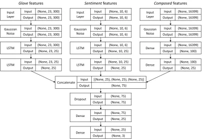
Figure 1 outlines the architecture of the neural network, which was implemented using Keras2. Unless specified otherwise, the hyper-parameters of each layer were set to their default value. The three input layers correspond, from left to right, to theGloVe,Sentiment, andComposed features. The first layer, which was applied to all the input layers, is a Gaussian Noise layer that introduces a noise of mean zero and average standard deviation defined as:

Gstdev =

1 N F

N F X

i=1

N I X

j=1

Xj,i−Xi

whereN F represents the number of features,N I the numbers of instances,Xj,i is the value of the

i-feature for thej-instance, andX¯i is the average value of thei-feature. From left to right, the average standard deviations for theGloVe,Sentiment, andComposedfeatures were approximately0.15,0.18, and

0.01. There were two reasons for using Gaussian Noise instead of a more traditional Dropout. Firstly, GloVeandSentimentfeatures could be seen as vectors representing concepts. Hence, adding Gaussian Noise can be seen as slightly changing the concept of a word hence working as data augmentation (Zhang and Yang, 2018), while Dropout introduces more drastic changes to the vector. Secondly, theComposed feature vectors are very sparse. For example, approximately 99.86% of the elements in the matrices representing both the Kumar’s training and validation datasets are zeros. Hence, Dropout would have had almost no impact in this representation. Then,GloVeandSentimentfeatures were processes by LSTM layers (Hochreiter and Schmidhuber, 1997), which are well-known for their capabilities for processing sequences. The last LSTM layers were set to return the last predicted value instead of a sequence. On

Input Layer

Input (None, 23, 300)

Output (None, 23, 300)

Gaussian Noise

Input (None, 23, 300)

Output (None, 23, 300)

Input Layer

Input (None, 10, 6)

Output (None, 10, 6)

Glove features Sentiment features Composed features

Input Layer

Input (None, 16399)

Output (None, 16399)

Gaussian Noise

Input (None, 10, 6)

Output (None, 10, 6)

Gaussian Noise

Input (None, 16399)

Output (None, 16399)

LSTM Input (None, 23, 300)

Output (None, 23, 25) LSTM

Input (None, 10, 6)

Output (None, 10, 25) Dense

Input (None, 16399)

Output (None, 100)

LSTM Input (None, 23, 25)

Output (None, 25) LSTM

Input (None, 10, 25)

Output (None, 25) Dense

Input (None, 100)

Output (None, 25)

Concatenate Input [(None, 25), (None, 25), (None, 25)] Output (None, 75)

Dropout Input (None, 75) Output (None, 75)

Dense Input (None, 75) Output (None, 25)

Dense Input (None, 25) Output (None, 3)

Figure 1: Neural Network

the other hand, theComposedfeatures were processed by dense layers. The first dense layer used arelu

activation, whereas the second one atanhactivation function. The goal was to constrain the elements in the output vector to values between−1 and1, which is also a constrain imposed by LSTM layers. Thereby, after concatenating the resulting outputs, no normalisation was needed. Then, to reduce a possible overfitting, a Dropout layer was applied, which set50% of the elements to zero. Finally, to get the predictions, anotherreluandsof tmaxactivated dense layer were applied. The neural network training considered a cross entropy loss function and weighted the classes using the “balanced” approach of scikit-learn3. Optimisation was based on a stochastic gradient descent with a learning rate of 0.01

and a momentum of0.1. The network was trained for600epochs. The selected neural network model corresponded to the one achieving the highest classification performance over the validation dataset.

Finally, the SVM considered theN-gram TF-IDF features and was trained using the scikit-learn im-plementation4. Parametrisation included a RBF (Radial Basis Function) kernel, in whichC was set to

1and gamma was set to0.4, according to the experimental evaluation performed over the training and validation sets. The SVM model was trained usingN-gram TF-IDF, which considers both word stems (i.e. word level features) and n-grams (i.e. character level features) because it obtained better results that using only n-grams or stems.

4 Results

This section describes the results obtained during the design phase of the proposed model (Section 4.1), as well as the results reported by the Shared Task on Aggression Identification organisers (Section 4.2).

4.1 Design phase results

This section outlines several experiments that were performed during the design phase to assess different feature extraction techniques and classifiers. Such techniques and classifiers were evaluated by not only

3

scikit-learn class weight: http://scikit-learn.org/stable/modules/generated/sklearn.utils. class_weight.compute_class_weight.html

4_{scikit-learn C-Support Vector Classification: http://scikit-learn.org/stable/modules/generated/}

0 0.1 0.2 0.3 0.4 0.5 0.6 0.7 0.8 0.9 1

Kumar et al. - Worst Result Kumar et al. - Best Result Reynolds et al. - Worst Result Reynolds et al. - Best Result Simple Feature Sets

Combination of Feature Sets

Word Embedding

Irony Detection Features

Submitted Model

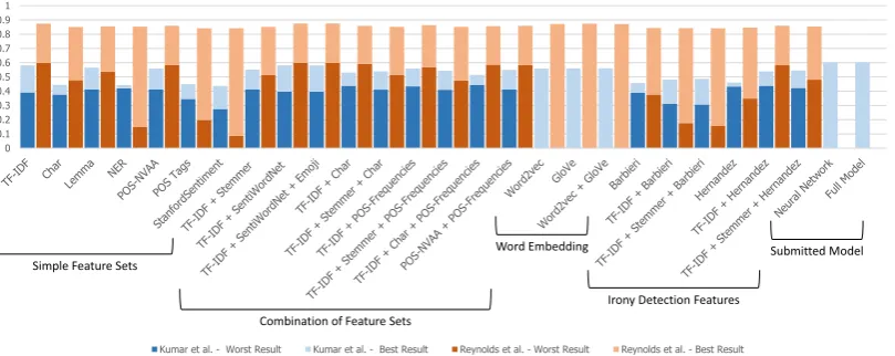
Figure 2: Design phase results

TF-IDF Tokenisation, stopword removal and TF-IDF weighting.

Stanford Sentiment Overall sentiment of the post and sentiment of each detected syntactic

structure.

Char The defined char-based features. word2vec Matrix representation based on word2vec.

Lemma Only the lemma of the tokenised terms are kept.

GloVe Matrix representation based on GloVe.

NER Only the recognised types of entities are

kept.. Barbieri

Irony detection features based on (Barbieri and Saggion, 2014).

POS-NVAA Only noun, verbs, adjectives and

adverbs are kept. Hernandez Irony detection features based on (Far´ıaset al., 2016).

POS Tags Instead of considering the actual terms,

it considers their POS tags. SentiWordNetTF-IDF +

TF-IDF + sentiment polarity of the post extracted with SentiWordnet.

POS-NVAA + POS-Frequencies

POS-NVAA + frequency of the different POS tags.

TF-IDF +

SentiWordNet + Emoji TF-IDF + Hernandez TF-IDF + Stemmer +Barbieri TF-IDF + Stemmer TF-IDF + Stemmer +

Hernandez TF-IDF + Barbieri word2vec + GloVe TF-IDF + Char TF-IDF + Stemmer +

Char

TF-IDF + POS Tags TF-IDF + Stemmer + POS Tags

TF-IDF + Char + POS Tags

Table 2: Feature Extraction

considering the dataset provided by Kumar et al. (2018b), but also the one provided by Reynolds et al. (2011). The latter dataset consists of approximately 3,000questions and answers collected from FormSpring.me5. In this social media site, users can post questions and answer other users’ questions with the option of anonymity. Posts were manually labelled into three categories: strongly aggressive, weakly aggressive and non-aggressive. According to the authors, the best classification achieved an overall accuracy of 81%, when considering features related to the number of curse words and their intensity. For Kumar et al.’s dataset, the training partition was used for training, while the validation partition was used for testing. As the Reynolds et al. dataset was not separated into training and test set, it was randomly split70%training and30%test sets. The worst and best results obtained using the described feature sets and classifiers are presented in Figure 2, as well as the results obtained for the models submitted to the challenge.

Table 2 summarises the selected feature sets for characterising aggression. Those feature sets (except-ing the word embedd(except-ing based features, i.e.,Word2VecandGloVe) were assessed considering multiple classification techniques, such as N¨aive Bayes, SVM with polynomial kernel, SVM with RBF kernel,

and fully connected shallow neural networks, i.e., a neural layer without hidden layers. N¨aive Bayes and SVM with polynomial kernel were consistently outperformed by the other techniques regardless the dataset and feature set under evaluation. Conversely, SVM with RBF kernel and fully connected shallow neural networks obtained the best results. Moreover, using a Batch Normalization layer improved the results of the neural network. Deeper dense neural networks were also tested, using up to 2 hidden layers. Nonetheless, they presented two drawbacks. First, the training phase required more than the available hardware resources. Second, in those cases in which the model could be trained, it overfitted the training set. Thereby, deeper neural networks were disregarded.Word2VecandGlovefeatures were tested using LSTM-based neural networks as these features are structured as a sequence of features rather than a set of features.

For all the evaluated combinations of feature sets and classification algorithms, results for Reynolds et al.’s dataset were higher than those of Kumar et al.’s dataset. Moreover, results varied at most3%for Raynolds et al.’s dataset, whilst for Kumar et al.’s dataset variations reached the34%. This difference could be caused by the fact that posts in Kumar et al.’s dataset were probably written by non native nor Occidental English speakers. Hence, it is likely to find many typos, misused slang, or unusual ex-pressions. Nonetheless, the different feature sets behaved similarly under both datasets. For instance, TF-IDF+SentiWordNet outperformed every other feature set, whist StanfordSentiment and POS tags achieved the worst performance for Reynolds et al.’s and Kumar et al.’s datasets, respectively. Interest-ingly, different types of features showed the same behaviour for both datasets. For example, considering simple textual features achieved for both datasets higher results than POS tags, lemmatisation, and word embeddings. Moreover, adding more features, such as addingChartoTD-IDF+POS-Frequencyor Emo-jistoTF-IDF+SentiWordNet, did not improve results, hinting that some features could introduce noise to post representation.

Finally, the statistical significance of results’ differences was tested. Since the data was shown not to be normal, a Wilcoxon test analysis for related samples was performed over the results for the differ-ent feature sets, where samples corresponded to the results for each classification algorithm. The null hypothesis stated that no difference existed amongst the results of the different samples, i.e. classifica-tion algorithms performed similarly regardless the feature set. Hence, the alternative hypothesis stated that the differences amongst the results obtained for each feature set were significant and non-incidental. In the case of Kumar et al., for most pairs of feature sets no statistically significant differences were observed with a confidence of0.01. Nonetheless, statistically significant differences were observed for BarbieriandStanfordSentiment, which were shown to be statistically lower than feature sets involving TF-IDF. On the other hand, in the case of Reynolds et al., no statistical differences were observed for the different feature sets. In brief, simple textual features, such asTF-IDF, seem to have the same descrip-tive capability than other more complex features for aggression detection using traditional classification techniques. However, further research is needed to confirm this hypothesis.

4.2 Challenge results

For the purpose of the First Shared Task on Aggression Identification, two sets of predictions were submitted for evaluation. The first set was generated considering the Neural Network described in Sec-tion 3.3, whilst the second one was generated using the full method described in that secSec-tion, i.e., the average between the Neural Network and the SVM model. Table 3 presents the F-measure obtained for the shared task, for both theFacebookandTwitterclassification tasks. The Random Baseline presented in this table was provided by the shared task organisation. Neural Network and Full Model are the re-sults forIsistanitos’models. Additionally, the last rows, for both tables present the results for the best performing models for each task. Similarly as for the design phase evaluations,Isistanitos’predictions were better for theFacebooktask. This situation highlights the differences amongst the different social media sites, and the effect that their particular characteristics have over the performed task.

System F1 (weighted)

Random Baseline 0.3535 Neural Network 0.5894 Full Model 0.5948

Best Performing (saroyehun) 0.6425

(a)FacebookTask

System F1 (weighted)

Random Baseline 0.3477 Neural Network 0.5369 Full Model 0.5480

Best Performing (vista.ue) 0.6009

(b)TwitterTask

Table 3: Results for the English task

OAG CAG NAG

Predicted label OAG

CAG

NAG

True label

68 59 17

15 87 40

60 217 353

Confusion Matrix

0.0 0.1 0.2 0.3 0.4 0.5 0.6

(a)FacebookTask

OAG CAG NAG

Predicted label OAG

CAG

NAG

True label

131 166 64

66 179 168

8 78 397

Confusion Matrix

0.0 0.1 0.2 0.3 0.4 0.5 0.6 0.7 0.8

(b)TwitterTask

Figure 3: Confusion matrices

that this distribution differs from the one of the train set (22.57%, 35.34%and42.09%, for the OAG, CAG and NAG classes, respectively), which could affect the predictive power of the trained models. On the other hand, for theTwitterset, the distribution was28.72%,32.86%and38.42%, for the OAG, CAG and NAG classes, respectively.

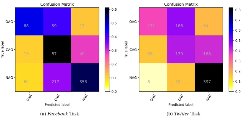
Table 4 shows the confusion matrices of the best submitted predictions per class and task. In the de-picted confusion matrices, one of the classes is considered the positive class and the other two are merged into the negative class, e.g. when analysing the NAG class, the posts actually belonging to that class are considering positive, whilst the posts belonging to CAG and OAG are regarded as negative. For the Facebooktask, NAG had a high True Positive Rate (TPR) of86.10%, but the True Negative Rate (TNR) was only of45.26%. For the other two classes, the TNR was higher than90%, but the TP was lower than

50%. Interestingly, the TPR for CAG was23.97%, evidencing that the classifier had severe problems to detect posts with covert aggressions. In contrast, when analysing theTwittertask, the TNR of each class was higher than the corresponding TPR. Particularly, the TNRs were86.31%,71.94%, and78.13%for NAG, CAG, and OAG respectively, whilst the TPRs were63.12%, 42.32%, and63.90%. Despite the different results observed for theFacebook andTwittertasks, it can be concluded that detecting covert aggressions is more difficult and error prone that the detection of explicit aggressions.

It is worth noting that detecting CAG posts resulted particularly challenging as they are written without openly using aggressive vocabulary. Moreover, the intent of such posts might be given by their context. Since the CAG class was originally defined as “an indirect attack against the victim and is often packaged as (insincere) polite expressions”, it might be necessary to know both reader and writer points of view to understand the real intention. As a result, detecting CAG posts might not be feasible if only the information regarding the individual posts is available.

Predicted

Negative Positive

ActualNAGClass Negative Positive

229 277 57 353

ActualCAGClass Negative Positive

498 55 75 68

ActualOAGClass Negative Positive

697 76 75 68

(a)FacebookTask

Predicted

Negative Positive

ActualNAGClass Negative Positive

542 86 232 397

ActualCAGClass Negative Positive

600 234 244 179

ActualOAGClass Negative Positive

822 230 74 131

(b)TwitterTask

Table 4: Error per class

0 0.1 0.2 0.3 0.4 0.5 0.6 0.7

Kumar et al. - FB Worst Result Kumar et al. - FB Best Result Kumar et al. - TW Worst Result Kumar et al. - TW Best Result

Simple Feature Sets

Combination of Feature Sets

Word Embedding

Irony Detection Features

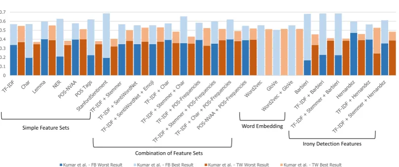
Figure 4:Facebook/Twittergold standard results

that could differ from those used by Occidental users, or with those presenting a more colloquial usage of English. Additionally, given the cultural differences, the criteria for defining what an aggression is and what it is not could differ, hence it could also occur that posts might have a hidden sense that the English language might not be able to capture. In this context, the performance of certain techniques and corpus commonly used for English natural language processing could be reduced.

Finally, after Kumar et al.’s gold standard was publicly released, the evaluations described in sec-tion 4.1 were repeated. In this case, Kumar et al.’s training and validasec-tion sets were both used for training, thus increasing the size of the training set, and testing was performed usingFacebookandTwittertesting sets. Figure 4 depicts the obtained results. When comparing these results with those obtained during the design phase (Figure 2) for the Kumar et al.’s dataset, theFacebook test set obtained better results in66%of the cases, with differences up to44%. This was expected as both Kumar et al.’s training and validation sets were purely gathered fromFacebook. However, such improvements were not statistically significant. This might be due to the fact that feature sets performed differently for the validation dataset. The Pearson correlation between the results obtained during the design phase and those for the Face-booktest set was−0.66(p-value<0.01). This implies that the greater improvements were observed for those feature sets that performed poorly during the design phase. For example,StanfordSentiment, which achieved the worst performance in the validation dataset, presented the best results for theFacebooktest set. On the other hand,TF-IDF+SentiWordNet, which obtained the best performance for the validation set, decreased its performance when considering the Facebook test set. In consequence, the negative correlation shows that it was particularly challenging to predict the performance of a feature set for the Facebooktest set from the validation set.

vali-dation dataset, such differences were statistically insignificant. Conversely than for the Facebook test set, the correlation between the validation and testTwitterresults was0.9(p-value<0.0001). Moreover, TF-IDF+SentiWordNet did not achieved the best results as for theFacebook test set, even achieving results a7.58%lower than lemmatisation (the best performing feature set). Since the Twitter test set has a similar class distribution to the original Kumar et al.’s training and validations sets, the observed performance might be linked to the class distribution. Nonetheless, more research is required to confirm this hypothesis.

As in section 4.1, a Wilcoxon test was performed with the results for bothFacebookandTwittertest set, defining the same hypotheses. When considering a confidence of0.01, the null hypothesis could not be rejected for any pair of feature sets. With a confidence of0.05, the null hypothesis could be rejected for some pair of features in both the Facebook (e.g. Barbieri and POS-NVAA, or StanfordSentiment andTD-IDF) and theTwitter(e.g. StanfordSentimentandBarbieri, orTF-IDFandPOS tags) test set. Interestingly, the pair of feature sets showing statistically significant differences differed according to the considered dataset. Since the same trained model was used for evaluating both datasets, it cannot be stated that any feature set was inherently superior to another feature set. Hence, further studies are required to assess the descriptive power of features.

5 Conclusions

Aggression in social media is a common issue currently affecting users. Considering the current rate of posting, it is infeasible to manually curate social networks. Therefore, automatic approaches to detect aggression are required, which need to be able to adapt to new aggressive behaviour as cyberaggressors modify their behaviours to avoid detection. It is worth noting that other important applications of the de-tection of aggressive content are the dede-tection of cyberextremism, cybercrime and cyberhate propaganda. This paper was developed in the context of the Shared Task of Aggression Detection (Kumar et al., 2018a), which focused on detecting aggression on social media textual content. The proposed approach integrated several textual representations including traditional character, word, sentiment and irony fea-tures, and state-of-the-art approaches, such as word embeddings. Results suggested that automatically detecting aggression is a rather complex task, specially when the aggression is covert. Since the shared task was at a post level granularity, information that might be relevant for the task was unavailable. For example, user profile (point of views, common expression, and general behaviour) and post context were both unknown.

Regarding future work, the consideration of new information sources, such as user profiles or context information could be explored. Other neural network architectures, such as CNN or BiLSTM, could also be explored in this context. Another line of work is studying unsupervised machine learning algo-rithms for feature generation. Considering that the presented approach is English specific, unsupervised algorithms might help to extend the model to different languages without requiring a new corpus from which to extract features. Finally, it could be analysed the adaptation of the proposed model to changes in language usage to cope with the ever evolving nature of social media sites.

Acknowledgements

We acknowledge the financial support provided by ANPCyT through PICT-2017-1459.

References

Swati Agarwal and Ashish Sureka. 2015. Applying social media intelligence for predicting and identifying on-line radicalization and civil unrest oriented threats. arXiv preprint arXiv:1511.06858.

Stefano Baccianella, Andrea Esuli, and Fabrizio Sebastiani. 2010. Sentiwordnet 3.0: An enhanced lexical resource for sentiment analysis and opinion mining. InProceedings of the Seventh conference on International Language Resources and Evaluation (LREC’10).

Despoina Chatzakou, Nicolas Kourtellis, Jeremy Blackburn, Emiliano De Cristofaro, Gianluca Stringhini, and Athena Vakali. 2017. Mean birds: Detecting aggression and bullying on twitter. InProceedings of the 2017 ACM on Web Science Conference, WebSci ’17, pages 13–22, New York, NY, USA. ACM.

Vikas S Chavan and Shylaja S S. 2015. Machine learning approach for detection of cyber-aggressive comments by peers on social media network. In2015 International Conference on Advances in Computing, Communications and Informatics (ICACCI), pages 2354–2358, Aug.

Delia Iraz´u Herna´ndez Far´ıas, Viviana Patti, and Paolo Rosso. 2016. Irony detection in twitter: The role of affective content. ACM Trans. Internet Technol., 16(3):19:1–19:24, July.

Sepp Hochreiter and J¨urgen Schmidhuber. 1997. Long short-term memory. Neural computation, 9(8):1735–1780.

Homa Hosseinmardi, Sabrina Arredondo Mattson, Rahat Ibn Rafiq, Richard Han, Qin Lv, and Shivakant Mishra. 2015. Analyzing labeled cyberbullying incidents on the instagram social network. In Tie-Yan Liu, Christie Napa Scollon, and Wenwu Zhu, editors,Social Informatics, pages 49–66, Cham. Springer International Publishing.

Clayton Hutto and Eric Gilbert. 2014. Vader: A parsimonious rule-based model for sentiment analysis of so-cial media text. InEighth International Conference on Weblogs and Social Media (ICWSM-14). Available at (20/04/16) http://comp. social. gatech. edu/papers/icwsm14. vader. hutto. pdf.

Petra Kralj Novak, Jasmina Smailovi´c, Borut Sluban, and Igor Mozetiˇc. 2015. Sentiment of emojis. PLoS ONE, 10(12):e0144296.

Ritesh Kumar, Atul Kr. Ojha, Shervin Malmasi, and Marcos Zampieri. 2018a. Benchmarking Aggression Identifi-cation in Social Media. InProceedings of the First Workshop on Trolling, Aggression and Cyberbulling (TRAC), Santa Fe, USA.

Ritesh Kumar, Aishwarya N. Reganti, Akshit Bhatia, and Tushar Maheshwari. 2018b. Aggression-annotated Corpus of Hindi-English Code-mixed Data. InProceedings of the 11th Language Resources and Evaluation Conference (LREC), Miyazaki, Japan.

Tomas Mikolov, Kai Chen, Greg Corrado, and Jeffrey Dean. 2013. Efficient estimation of word representations in vector space. arXiv preprint arXiv:1301.3781.

Chikashi Nobata, Joel Tetreault, Achint Thomas, Yashar Mehdad, and Yi Chang. 2016. Abusive language detec-tion in online user content. InProceedings of the 25th International Conference on World Wide Web, WWW ’16, pages 145–153. International World Wide Web Conferences Steering Committee.

Jeffrey Pennington, Richard Socher, and Christopher D. Manning. 2014. Glove: Global vectors for word repre-sentation. InEmpirical Methods in Natural Language Processing (EMNLP), pages 1532–1543.

Martin Porter. 1980. An algorithm for suffix stripping.Program, 14(3):130–137.

Kelly Reynolds, April Kontostathis, and Lynne Edwards. 2011. Using machine learning to detect cyberbullying. In2011 10th International Conference on Machine Learning and Applications and Workshops, volume 2, pages 241–244, Dec.

Semiu Salawu, Yulan He, and Joanna Lumsden. 2017. Approaches to automated detection of cyberbullying: A survey. IEEE Transactions on Affective Computing, In press.

Cynthia Van Hee, Els Lefever, Ben Verhoeven, Julie Mennes, Bart Desmet, Guy De Pauw, Walter Daelemans, and Veronique Hoste. 2015. Automatic detection and prevention of cyberbullying. In Pascal Lorenz and Christian Bourret, editors,International Conference on Human and Social Analytics, Proceedings, pages 13–18. IARIA.

Elizabeth Whittaker and Robin M. Kowalski. 2015. Cyberbullying via social media. Journal of School Violence, 14(1):11–29.

Dongxu Zhang and Zhichao Yang. 2018. Word embedding perturbation for sentence classification. CoRR, abs/1804.08166.