Gradient Density Estimation in Arbitrary Finite Dimensions Using the Method of Stationary Phase

ISSN Online: 2160-0384 ISSN Print: 2160-0368

DOI: 10.4236/apm.2019.912051 Dec. 24, 2019 1034 Advances in Pure Mathematics

Gradient Density Estimation in Arbitrary Finite

Dimensions Using the Method of Stationary

Phase

Karthik S. Gurumoorthy

1

, Anand Rangarajan

2*

, John Corring

3

1_{International Center for Theoretical Sciences, Tata Institute of Fundamental Research, Bengaluru, Karnataka, India} 2_{Department of Computer and Information Science and Engineering, University of Florida, Gainesville, Florida, USA} 3_{Microsoft Research, Seattle, Washington, USA}

Abstract

We prove that the density function of the gradient of a sufficiently smooth function _S:_{Ω ⊂}d_{→, obtained via a random variable transformation of} a uniformly distributed random variable, is increasingly closely approximated by the normalized power spectrum of

φ

exp iS

τ

 

= _{ }

  as the free parameter 0

τ

→ _{. The frequencies act as gradient histogram bins. The result is shown} using the stationary phase approximation and standard integration tech-niques and requires proper ordering of limits. We highlight a relationship with the well-known characteristic function approach to density estimation, and detail why our result is distinct from this method. Our framework for computing the joint density of gradients is extremely fast and straightforward to implement requiring a single Fourier transform operation without expli-citly computing the gradients.

Keywords

Stationary Phase Approximation, Density Estimation, Fourier Transform, Wave Functions, Characteristic Functions

1. Introduction

Density estimation methods provide a faithful estimate of a non-observable probability density function based on a given collection of observed data [1][2] [3][4]. The observed data are treated as random samples obtained from a large population which is assumed to be distributed according to the underlying

den-How to cite this paper: Gurumoorthy, K.S., Rangarajan, A. and Corring, J. (2019) Gradient Density Estimation in Arbitrary Finite Dimensions Using the Method of Stationary Phase. Advances in Pure Ma-thematics, 9, 1034-1058.

https://doi.org/10.4236/apm.2019.912051

Received: November 13, 2019 Accepted: December 21, 2019 Published: December 24, 2019

Copyright © 2019 by author(s) and Scientific Research Publishing Inc. This work is licensed under the Creative Commons Attribution International License (CC BY 4.0).

http://creativecommons.org/licenses/by/4.0/

DOI: 10.4236/apm.2019.912051 1035 Advances in Pure Mathematics sity function. The aim of our current work is to show that the joint density func-tion of the gradient of a sufficiently smooth funcfunc-tion S (density function of ∇S₎ can be obtained from the normalized power spectrum of

φ

exp iS

τ

 

= _{ }

  as the free parameter τ _{tends to zero. The proof of this relationship relies on the} higher order stationary phase approximation [5]-[10]. The joint density function of the gradient vector field is usually obtained via a random variable transforma-tion, of a uniformly distributed random variable X over the compact domain

d

Ω ⊂_{ , using} ∇S _{as the transformation function. In other words, if we define} a random variable Y = ∇S X

( )

where the random variable X has a uniform distribution on the domain Ω ₍X UNI

( )

Ω ), the density function of Y

represents the joint density function of the gradient of S.

In computer vision parlance—a popular application area for density estima-tion—these gradient density functions are popularly known as the histogram of oriented gradients (HOG) and are primarily employed for human and object detection [11][12]. The approaches developed in [13][14] demonstrate an ap-plication of HOG—in combination with support vector machines [15]—for de-tecting pedestrians from infrared images. In a recent article [16], an adaption of the HOG descriptor called the Gradient Field HOG (GF-HOG) is used for sketch-based image retrieval. In these systems, the image intensity is treated as a function S X

( )

over a 2D domain, and the distribution of intensity gradients or edge directions is used as the feature descriptor to characterize the object ap-pearance or shape within an image. In Section 5 we provide experimental evi-dence to showcase the efficacy of our method in computing the density of these oriented gradients (HOG). The present work has also been influenced by recent work on quantum supremacy [17][18] [19]. Here, the aim is to draw samples from the density function of random variables corresponding to the measure-ment bases of a high-dimensional quantum mechanical wave function. This work may initially seem far removed from our efforts. However, as we will show, the core of our density estimation approach is based on evaluating interval measures of the squared magnitude of a wave function in the frequency domain. For this reason, our approach is deemed a wave function approach to density es-timation and henceforth we refer to it as such.

va-DOI: 10.4236/apm.2019.912051 1036 Advances in Pure Mathematics nishing Hessian problem. The reader may refer to [20] for a more detailed ex-planation. In contrast to our previous work, we regard our current effort as a generalization of the gradient density estimation result, now established for ar-bitrary smooth functions in arbitrary finite dimensions.

1.1. Main Contribution

We introduce a new approach for computing the density of Y, where we express the given function S as the phase of a wave function

φ

, specifically

( )

exp iS

( )

φ

τ

 

=  

 

x

x for small values of τ_{, and then consider the normalized}

power spectrum—squared magnitude of the Fourier transform—of

φ

[21]. We show that the computation of the joint density function of Y = ∇S _{may be} ap-proximated by the power spectrum of

φ

, with the approximation becoming in-creasingly tight point-wise as

τ

→0_{. Using the stationary phase approximation,} a well known technique in asymptotic analysis [9], we show that in the limiting case as

τ

→0_{, the power spectrum of}

φ

_{converges to the density of Y, and}

hence can serve as its density estimator at small, non-zero values of τ . In other words, if P

( )

u denotes the density of Y, and if Pτ

( )

u corresponds to the

power spectrum of

φ

at a given value of τ , Theorem 3.2 constitutes the fol-lowing relation,

( )0

( )

( )0

( )

0

lim P d P d

η η

τ

τ →

∫

=

∫

u u

u u u u

 

where η

( )

u0 is a small neighborhood around u0. We would like to

em-phasize that our work is fundamentally different from estimating the gradient of a density function [22] and should not be semantically confused with it.

1.2. Significance of Our Result

As mentioned before, the main objective of our current work is to generalize our effort in [20] and demonstrate the fact that the wave function method for ob-taining densities can be extended to arbitrary functions in arbitrary finite di-mensions. However, one might broach a legitimate question, namely “Whatis theprimaryadvantageof thisapproach overothersimpler, effectiveand tradi-tional techniques like histograms which can compute the HOG say bymildly smoothingtheimage, computingthegradientvia (forexample) finitedifferences andthenbinningtheresultinggradients?”. The benefits are three fold:

 One of the foremost advantages of our wave function approach is that it re-covers the joint gradient density function of Swithout explicitly computing its gradient. Since the stationary points capture gradient information and map them into the corresponding frequency bins, we can directly work with

S without the need to compute its derivatives.

 _{The significance of our work is highlighted when we deal with the more}

DOI: 10.4236/apm.2019.912051 1037 Advances in Pure Mathematics of the complete description of S on Ω_{. Given the N samples of S on} Ω_{, it} is customary to know the approximationerror of a proposed density estima-tion method as N→ ∞. In [23] we prove that in one dimension, the point-wise approximation error between our wave function method and the true density is bounded above by O N

(

1

)

when τ ∝1N . For histograms and kernel density estimators [1] [2], the approximation errors are estab-lished for the integrated mean squared error (IMSE) defined as the expected value (with respect to samples of size N) of the square of the 2 error

be-tween the true and the computed probability densities and are shown to be

2 3

O N_ − _

  [24] [25] and

4 5

O N_ − _

  [26] respectively. Having laid the foun-dation in this work, we plan to invest our future efforts in pursuit of similar upper bounds in arbitrary finite dimensions.

 Furthermore, obtaining the gradient density using our framework in the fi-nite N sample setting is simple, efficient, and computable in O N

(

logN

)

time as elucidated in the last paragraph of Section 4.

1.3. Motivation from Quantum Mechanics

Our wave function method is motivated by the classical-quantum relation, wherein classical physics is expressed as a limiting case of quantum mechanics [27][28]. When S is treated as the Hamilton-Jacobi scalar field, the gradients of

S correspond to the classical momentum of a particle [29]. In the parlance of quantum mechanics, the squared magnitude of the wave function expressed ei-ther in its position or momentum basis corresponds to its position or momen-tum density respectively. Since these representations (either in the position or momentum basis) are simply (suitably scaled) Fourier transforms of each other, the squared magnitude of the Fourier transform of the wave function expressed in its position basis is its quantum momentum density. However, the time inde-pendent Schrödinger wave function φ

( )

x (expressed in its position basis) can be approximated by exp iS

( )

τ

 

 

 

x

as

τ

→0 _{[28]. Here} τ _{(treated as a free} parameter in our work) represents Planck’s constant. Hence the squared magni-tude of the Fourier transform of exp iS

( )

τ

 

 

 

x

corresponds to the quantum

momentum density of S. The principal results proved in the article state that the classical momentum density (denoted by P) can be expressed as a limiting case (as

τ

→0) of its corresponding quantum momentum density (denoted by Pτ),

in agreement with the correspondence principle.

DOI: 10.4236/apm.2019.912051 1038 Advances in Pure Mathematics Let x denote the Hessian of S at a location x∈ Ω and let det

( )

x denote its determinant. The signature of the Hessian of S at x, defined as the differ-ence between the number of positive and negative eigenvalues of x, is represented by σ_{x. In order to exactly determine the set of locations where the} joint density of the gradient of S exists, consider the following three sets:

( )

{

: S

}

,

= ∇ =

u x x u

 (2.1)

( )

{

: det 0 ,

}

= x _x =

  (2.2)

and

( )

{

S :

}

.

= ∇ x x∈ ∂Ω

  (2.3)

Let N

( )

u = _u . We employ a number of useful lemma, stated here and proved in Appendix A.

Lemma 2.1. [FinitenessLemma] u isfiniteforevery u∉.

As we see from Lemma 2.1 above, for a given u∉, there is only a finite col-lection of x∈ Ω that maps to u under the function ∇S. The inverse map

( )1

_{( )}

S−

∇ u which identifies the set of x∈ Ω that maps to u under ∇S _is ill-defined as a function as it is a one to many mapping. The objective of the fol-lowing lemma (Lemma 2.2) is to define appropriate neighborhoods such that the inverse function _∇S( )−1_{, required in the proof of our main Theorem 3.2, when}

restricted to those neighborhoods is well-defined.

Lemma 2.2. [NeighborhoodLemma] Forevery u0∉, thereexistsaclosed

neighborhood η

( )

u0 around u0 such that η

( )

u0  is empty.

Fur-thermore, if _u0 >0, η

( )

u0 canbechosensuchthatwecanfindaclosed

neighborhood η

( )

x around each x∈u0 satisfying the following

condi-tions:

1) ∇S

(

η

( )

x

)

=η

( )

u0 .

2) det

( )

y ≠ ∀ ∈0, y η

( )

x .

3) The inverse function ( )1

_{( )}

_{( )}

_{( )}

0

:

S− η η

∇ _x u  u → x is well-defined. 4) For y z, ∈η

( )

x,σy =σz.

Lemma 2.3 [DensityLemma] Given X UNI

( )

Ω , theprobabilitydensityof

( )

Y= ∇S X _{on }d _{− isgivenby}

( )

_{( )}

( )

( )

1

1 1

det _k N

k P

µ

=

=

Ω

∑

u

x

u

 (2.4)

where xk∈u,∀ ∈k

{

1,2, , N

( )

u

}

and

µ

is the Lebesgue measure.

DOI: 10.4236/apm.2019.912051 1039 Advances in Pure Mathematics (S C_∈ ∞

( )

_{Ω ) can be relaxed to functions S in C}d2+1

( )

_{Ω where d is the}

dimen-sionality of Ω _{as we will see in Section 3.2.2.}

3. Equivalence of the Densities of Gradients and the Power

Spectrum

Define the function _F : d

τ  → as

( )

(

) ( )

2 12

( )

1 _{exp d}

2 d

i

Fτ

_τ

S

τ µ

Ω

 

= _ _ − ⋅ _

π Ω

∫

 

u x u x x (3.1)

or

τ

>0 . Fτ is very similar to the Fourier transform of the function

( )

exp iS

τ

 

 

 

x

. The normalizing factor in Fτ comes from the following lemma

(Lemma 3.1) whose proof is given in Appendix A. Lemma 3.1. [IntegralLemma ] _{F L}2

( )

d

τ∈  and Fτ ₂=1.

The power spectrum defined as

( )

( ) ( )

Pτ u ≡Fτ u Fτ u (3.2)

equals the squared magnitude of the Fourier transform. Note that Pτ ≥0. From Lemma (3.1), we see that

∫

Pτ

( )

u ud =1. Our fundamental contribution lies in

interpreting Pτ

( )

u as a density function and showing its equivalence to the

density function P

( )

u defined in (2.4). Formally stated: Theorem 3.2. For u0∉,

( )

(

)

( )0

( )

( )

0

0 0

0

1

lim lim P d P

α

τ

α τ

α

µ

→ →

∫

=

u

u u u

u 



where α

( )

u0 is a ball around u0 of radius α.

Before embarking on the proof, we would like to emphasize that the ordering of the limits and the integral as given in the theorem statement is crucial and cannot be arbitrarily interchanged. To press this point home, we show below that after solving for Pτ , the limτ→0Pτ does not exist. Hence, the order of the

integral followed by the limit

τ

→0 cannot be interchanged. Furthermore, when we swap the limits of α _and τ _{, we get}

( )

(

)

( )0

( )

( )

0

0 0 0

0

1

lim lim P d limP

α

τ τ

τ α τ

α

µ

→ →

∫

= →

u

u u u

u 



which also does not exist. Hence, the theorem statement is valid only for the specified sequence of limits and the integral.

3.1. Brief Exposition of the Result

To understand the result in simpler terms, let us reconsider the definition of the

scaled Fourier transform given in (3.1). The first exponential exp iS

( )

τ

 

 

 

x

is a

varying complex “sinusoid”, whereas the second exponential exp i

τ

⋅

₋ 

 

 

DOI: 10.4236/apm.2019.912051 1040 Advances in Pure Mathematics fixed complex sinusoid at frequency _τu. When we multiply these two complex

exponentials, at low values of τ _{, the two sinusoids are usually not “in sync” and} tend to cancel each other out. However, around the locations where ∇S

( )

x =u, the two sinusoids are in perfect sync (as the combined exponent is stationary) with the approximate duration of this resonance depending on det

( )

x . The value of the integral in (3.1) can be increasingly closely approximated via the sta-tionary phase approximation [9] as

( )

( )

( )

( )

( )

1 1 2

1 1 _{exp .}

4

det _k k

N u

k k

k

i

Fτ _τ S iσ

µ =

 _{ } 

≈ _{ } − ⋅ _+ _

 

Ω

π

∑

x

x

u x u x



The approximation is increasingly tight as τ →0. The power spectrum (Pτ)

gives us the required result

_{( )}

( )

( )

1

1 1

det _k

N u k

µ _Ω

∑

=

x

 except for the cross phase factors S

( )

xk −S

( )

xl − ⋅u x

(

k−xl

)

obtained as a byproduct of two or more

remote locations xk and xl indexing into the same frequency bin u, i.e., k ≠ l

x x , but ∇S

( )

xk = ∇S

( )

xl =u. The cross phase factors when evaluated are

equivalent to cos 1

τ

   

 , the limit of which does not exist as

τ

→0. However, integrating the power spectrum over a small neighborhood α

( )

u around u

removes these cross phase factors as τ _{tends to zero and we obtain the desired} result.

3.2. Formal Proof of Theorem 3.2

We wish to compute the integral

( )

(

) ( )

2 12

(

( )

)

1 _{exp d}

2 d

i

Fτ

_τ

S

τ µ

Ω

 

= _ − ⋅ _

 

Ω

π

∫

u x u x x (3.3)

at small values of τ and exhibit the connection between the power spectrum

( )

Pτ u and the density function P

( )

u . To this end define

(

;

)

S

( )

Ψ x u ≡ x − ⋅u x. The proof follows by considering two cases: the first case in which there are no stationary points and therefore the density should go to zero, and the second case in which stationary points exist and the contribution from the oscillatory integral is shown to increasingly closely approximate the density function of the gradient as

τ

→0_.

re-DOI: 10.4236/apm.2019.912051 1041 Advances in Pure Mathematics lationship to stationary points of the second kind to Appendix 8.) Under mild conditions (outlined in Appendix B), the contributions from the stationary points of the third kind can also be ignored as they approach zero as τ tends to zero [9]. Higher order terms follow suit.

Lemma 3.3. Fix u0∉.If u0 = ∅ then Fτ

( )

u0 =O

( )

τ

as

τ

→0.

Proof. To improve readability, we prove Lemma 3.3 first in the one dimen-sional setting and separately offer the proof for multiple dimensions.

3.2.1. Proof of Lemma 3.3 in One Dimension

Let s denote the derivative (1D gradient) of S. The bounded closed interval Ω is represented by Ω =

[

b b1, 2

]

, with the length L=µ

( )

Ω =b b2− 1. As u0∉,

there is no x∈ Ω _{for which} s x

( )

=u0. Recalling the definition of Ψ, namely

( )

x u; S x ux

( )

Ψ ≡ − _{, we see that} Ψ′

( )

x ≠0 _{and is of constant sign in}

[

b b₁, ₂

]

. It follows that Ψ

( )

x is strictly monotonic. Defining v= Ψ

( )

x , we have from (3.1)

( )

_{( )}( )2

( )

1

0 1 exp d .

2

b b

iv

F u t v v

L τ

_τ

τ

Ψ Ψ       π =

_∫

Here

( )

( )

(

1

)

1 t v v − = ′

Ψ Ψ . The inverse function is guaranteed to exist due to the monotonicity of Ψ_{. Integrating by parts we get}

( )

( )

(

( )

)

( )

(

( )

)

( )

( )2

_{( )}

1

2 1

0 2 exp 2 exp 1

exp d .

b b

i b i b

F u L t b t b

i

iv t v v i

τ τ τ _{τ τ}

τ

τ

Ψ Ψ

  Ψ   Ψ  

=    Ψ −   Ψ 

          ′_  π − _ 

∫

(3.4)

It follows that

( )

_{( )}

_{( )}

_{( )}( )2

( )

1 0

2 0 1 0

1 1 _{d .}

2

b b

F u t v v

s b u s b u L τ

τ

Ψ Ψ   ′ ≤ _ + +  − 

π −

∫

_

3.2.2. Proof of Lemma 3.3 in Finite Dimensions As ∇Ψ

(

x u; 0

)

≠ ∀0, x, the vector field

( )

1 2 ∇Ψ = ∇Ψ v x

is well-defined. Choose 2 d

m> _{(with this choice explained below) and for}

{

1,2, ,

}

j∈  m , recursively define the function gj

( )

x and the vector field

( )

1 j+

v x as follows:

( )

1 1,

g x =

( )

( )

1

j j

g + x = ∇ ⋅v x

and

( )

( )

1 2 1 .

j+ gj+

∇Ψ =

∇Ψ

DOI: 10.4236/apm.2019.912051 1042 Advances in Pure Mathematics Using the equality

(

)

( )

( )

(

)

( )

(

)

0

0 0

exp ;

exp ; exp ;

j

j j

i _g

i i

i i

τ

τ τ

τ τ

 _Ψ 

 

 

 

   

 

= _∇ ⋅ _{ } Ψ _− ∇ ⋅_{ } Ψ _

    

x u x

v x x u v x x u

(3.5)

where ∇ ⋅ _{is the divergence operator, and applying the divergence theorem m} times, the Fourier transform in (3.3) can be rewritten as

( )

(

) ( )

( )

( )

( )

(

) ( )

( )

(

( )

)

(

( )

)

0 1 1

2 2

1 1 2 2

1 _{exp d}

2

1 _{exp d}

2

m m d

m _j

j d

j

i

F i g

i i

τ τ _τ

τ µ

τ

τ τ µ

+ Ω

= ∂Ω

 

= _ Ψ _

 

Ω

 

 

− _ ⋅ _{ } Ψ _

π

 

Ω π

∫

∑

∫

u x x x

v x y n x y y

(3.6)

which is similar to (3.4).

We would like to add a note on the differentiability of S which we briefly mentioned after Lemma 2.3. The divergence theorem is applied

2 d

m> _times to obtain sufficiently higher order powers of τ _{in the numerator so as to} exceed the _τ2d _{term in the denominator of the first line of (3.6). This}

necessi-tates that S is at least 1 2

d _{+ times differentiable. The smoothness constraint on}

S can thus be relaxed and replaced by 2 1

( )

d

S C∈ + Ω _.

The additional complication of the d-dimensional proof lies in resolving the geometry of the terms in the second line of (3.6). Here n is the unit outward normal to the positively oriented boundary ∂Ω parameterized by y. As

2 d

m> _{, the term on the right side of the first line in (3.6) is} o

( )

τ

and hence can be overlooked. To evaluate the remaining integrals within the summation in (3.6), we should take note that the stationary points of the second kind for

( )

Ψ x on Ω _{correspond to the first kind of stationary points for} Ψ

(

x y

( )

)

on the boundary ∂Ω_{. We show in case (ii) that the contribution of a stationary} point of the first kind in a d−1 _{dimensional space is} 21

d O_

τ

− _

 . As the dimension of ∂Ω _is d−1_{, we can conclude that the total contribution from}

the stationary points of the second kind is 21

d O_

τ

− _

 . After multiplying and

di-viding this contribution by the corresponding _τj _{and τ}2d _{factors respectively,}

it is easy to see that the contribution of the jth _{integral (out of the n integrals in}

the summation) in (3.6) is _O_

_τ

j−12_

 

 , and hence the total contribution of the m integrals is of O

( )

τ

_{. Here, we have safely ignored the stationary points of the}

DOI: 10.4236/apm.2019.912051 1043 Advances in Pure Mathematics as shown in [9]. Combining all the terms in (3.6) we get the desired result, namely F uτ

( )

0 =O

( )

τ

. For a detailed exposition of the proof, we encourage

the reader to refer to Chapter 9 in [9].

We then get Pτ

( )

u0 =O

( )

τ . Since ∇ ΩS

( )

is a compact set in d and

( )

0∉∇ ΩS

u , we can choose a neighborhood η

( )

u0 around u0 such that

for u∈η

( )

u0 , no stationary points exist and hence

( )0

( )

0

lim P d 0.

η

τ

τ→

∫

=

u

u u



Since the cardinality N

( )

u of the set u defined in (2.1) is zero for

( )

0

η

∈

u  u , the true density P

( )

u of the random variable transformation

( )

Y= ∇S X given in (2.4) also vanishes for u∈η

( )

u0 .

case (ii): For u0∉, let N

( )

u0 >0. In this case, the number of stationary

points in the interior of Ω _{is non-zero and finite as a consequence of Lemma} 2.1. We can then rewrite

( )

(

) ( )

( )

( )

(

)

0

0 1 0

1

2 2

1 _{exp ; d}

2 k N d k i F G η τ

_τ

τ µ

=

 

= + _ Ψ _

 

Ω

π

∑ ∫

u

x

u x u x



, (3.7)

where

(

0

)

exp ; d

K i G

τ

 

≡ _ Ψ _

 

∫

x u x (3.8)

and the domain ( )0

( )

1

\N _k

k

K η

=

≡ Ω

_

u  x . The closed regions

{

( )

}

( )0

1 N k k η ₌ u x

 are

obtained from Lemma 2.2.

Firstly, note that the the set K contains no stationary points by construction. Secondly, the boundaries of K can be classified into two categories: those that overlap with the sets η

( )

xk and those that coincide with Γ = ∂Ω. Propi-tiously, the orientation of the overlapping boundaries between the sets K and each η

( )

xk are in opposite directions as these sets are located at different

sides when viewed from the boundary. Hence, we can exclude the contributions from the overlapping boundaries between K and η

( )

xk while evaluating

( )

0

Fτ u in (3.7) as they cancel each other out.

To compute G we leverage case (i), which also includes the contribution from the boundary Γ_{, and get}

(

)

( )

1 0, .

G= u

τ

=O

τ

(3.9)

To evaluate the remaining integrals over η

( )

xk , we take into account the

contribution from the stationary point at xk and obtain

( )

(

)

(

)

( )

(

)

(

)

0 2

0 2 0

exp ; d

2

exp ; , ,

4 det k k k d k i

a i _i

η τ

τ

σ τ

τ  _Ψ 

 

 

 

= _ Ψ + _+

 π  π

∫

x x x

x u x

x u u



 

DOI: 10.4236/apm.2019.912051 1044 Advances in Pure Mathematics where

(

)

21 21

( )

2 0, 1 0

d d

O

τ

= _

τ

+ _≤

τ γ

+

 

u u

 (3.11)

for a continuous bounded function γ1

( )

u [9]. The variable a in (3.10) takes the

value 1 if xk lies in the interior of Ω, otherwise equals 1₂ if xk∈ ∂Ω. Since ∉

u , stationary points do not occur on the boundary and hence a=1 for our case. Recall that σ_xk is the signature of the Hessian at xk. Note that the main term has the factor _τd2 _{in the numerator, when we perform stationary phase in}

d dimensions, as mentioned under the finite dimensional proof of Lemma 3.3. Coupling (3.7), (3.8), and (3.10) yields

( )

( )

( )

(

)

( )

(

)

0

0 1 0 3 0

1 2

1 _{exp ;} 1 _,

4 _det k k N k k i

Fτ _τ iσ τ

µ =

 

= _ Ψ + _ +

 

Ω

π

∑

u x

x

u x u  u

 (3.12)

where

(

)

(

)

(

)

(

) ( )

2 0

3 0 1 0 1

2 2 , , , . 2 d τ τ τ τ µ π = + Ω u

u u 

 

As 1

(

u0,

τ

)

=O

( )

τ

and

(

)

1 2 2 0,

d O

τ

= _

τ

+ _

 

u

 from (3.9) and (3.11)

re-spectively, we have 3

(

u0,

τ

)

=O

( )

τ

. Based on the definition of the power

spectrum Pτ in (3.2), we get

( )

_{( )}

( )

( )

( )

( ) ( )

(

)

(

)

(

)

( )

( )

(

)

0 0 0 0 1 0 0 1 1 4 0 1 1 det

exp ; ;

1 4 det det , k k l k l N k

N N k l

l k l k P i _i τ _µ σ σ τ µ τ = = = ≠ = Ω

 _{Ψ − Ψ + −} 

 _{ } π

  + Ω +

∑

∑ ∑

u x

u u x x

x x

u

x u x u

u



 



(3.13)

where 4

( )

u0 includes both the squared magnitude of 3

(

u0,τ

)

and the cross

terms involving the first term in (3.12) and 3

(

u0,τ

)

. Notice that the main term

in (3.12) can be bounded independently of τ _as

(

0

)

exp ; 1, 0

4

k k

i _{iσ τ}

τ

 _{Ψ +}  _{= ∀ ≠}

 π_

 x u x

and det

( )

_xk ≠ ∀0, k. Since 3

(

u0,

τ

)

=O

( )

τ

, we get 4

(

u0,

τ

)

=O

( )

τ

.

Furthermore, as 4

(

u0,τ

)

can also be uniformly bounded by a function of u

for small values of τ_{, we have}

( )0

(

)

4 0

0

lim , d 0.

η

τ→

∫

τ

=

u

u u



 (3.14)

DOI: 10.4236/apm.2019.912051 1045 Advances in Pure Mathematics anticipated expression for the density function P u

( )

0 given in (2.4). The cross

phase factors in the second line of (3.13 arise due to multiple remote locations k

x and xl indexing into u. The cross phase factors when evaluated can be shown to be proportional to cos 1

τ

   

 . Since 0 1 limτ→ cos  

_τ

  is not defined,

( )

0 0

limτ→ Pτ u does not exist. We briefly alluded to this problem immediately

following the statement of Theorem 3.2 in Section 3. However, the following lemma which invokes the inverse function ( )1

( )

( )

( )

0

:

S− η η

∇ _x u  u → x —defined in Lemma 2.2 where x is written as a function of u—provides a simple way to nullify the cross phase factors. Note that since each _∇S( )−1

x is a bijection, N

( )

u doesn’t vary over η

( )

u0 . Pursuant to Lemma 2.2, the

Hes-sian signatures σx u_{k( )} and σx ul( ) also remain constant over η

( )

u0 .

Lemma 3.4. [CrossFactorNullifierLemma] Theintegralofthecrosstermin the second line of (3.13) over the closed region η

( )

u0 approacheszero as

0

τ

→ _{, i.e.,}

∀ ≠

k l

( )

( )

(

)

(

( )

)

( )

(

)

(

( )

)

0

1 1

0

2 2

exp ; ;

lim d 0.

det _k det _l

k l

i

η

τ

τ

→

 _{Ψ − Ψ }

 _{ }

  ₌

∫

u

x u x u

x u u x u u

u

 _{ }

(3.15)

The proof is given in Appendix A. Combining (3.14) and (3.15) yields

( )

( )

( )

( ) ( )

( )

(

)

( )

( )

0 0 0

0 ₁

1 1

lim d d d .

det _k

N k

P P

η η η

τ

τ→

∫

=µ Ω

∫

∑

₌ =

∫

u

u u _{x u} u

u u u u u

   

(3.16)

Equation (3.16) demonstrates the equivalence of the cumulative distributions corresponding to the densities Pτ

( )

u and P

( )

u when integrated over any sufficiently small neighborhood η

( )

u0 of radius

η

. To recover the density

( )

P u , we let

α η

< and take the limit with respect to α .

Taking a mild digression from the main theme of this paper, in the next sec-tion (Secsec-tion 4), we build an informal bridge between the commonly used cha-racteristic function formulation for computing densities and our wave function method. The motivation behind this section is merely to provide an intuitive reason behind our Theorem 3.2, where we directly manipulate the power spectrum of φ

( )

exp iS

( )

τ

 

=  

 

x

x into the characteristic function formulation

cha-DOI: 10.4236/apm.2019.912051 1046 Advances in Pure Mathematics racteristic function methods as two different approaches for estimating the probability density functions and not reformulations of each other. To press this point home, we also comment on the computational complexity of the wave function and the characteristic function methods at the end of the next section.

4. Relation between the Characteristic Function and Power

Spectrum Formulations of the Gradient Density

The characteristic function ψY

( )

w for the random variable Y = ∇S X

( )

is

defined as the expected value of exp

(

i Yw⋅

)

, namely

( )

exp

(

)

_{( )}

1 exp

(

( )

)

d .

Y E i Y i S

ψ

µ Ω

≡ _ ⋅ _= ⋅∇ Ω

∫

w w w x x (4.1)

Here _µ

_{( )}

1_Ω denotes the density of the uniformly distributed random variable

X on Ω_.

The inverse Fourier transform of a characteristic function also serves as the density function of the random variable under consideration [30]. In other words, the density function P

( )

u of the random variable Y can be obtained via

( )

( )

( )

(

)

( ) ( )

(

( )

)

1 _{exp d}

2

1 _{exp d d .}

2

Y d

d

P i

i S

ψ ω

µ Ω

π

= − ⋅

= ⋅ ∇_ − _ π Ω

∫

∫∫

u w u w

w x u x w (4.2)

Having set the stage, we can now proceed to highlight the close relationship between the characteristic function formulation of the density and our formula-tion arising from the power spectrum. For simplicity, we choose to consider a region Ω _{that is the product of closed intervals,}

[

]

1

, d

i i i

a b

=

Ω =

∏

_{. Based on the}

expression for the scaled Fourier transform Fτ

( )

u in (3.1), the power spec-trum Pτ

( )

u is given by

( )

(

2

) ( )

1d exp

( ) ( )

(

(

)

)

d d . i

Pτ _τ S S

τ µ Ω Ω

 _{ }

= _{ } − − ⋅ − _

 

Ω

π

∫ ∫

u x y u x y x y

Define the following change of variables,

, .

2

τ

− +

= x y = x y

ω

ν

Then ,

2 2

τ τ

= + = −

x ν ω y ν ω _{and the integral limits for} ω and ν _{are given} by

1

,

d

i i i i

i

a b b a W

τ τ

=

− −

 

= _{ }

 

∏

1 2 , 2

d

i i

i i

i

V a

ω τ

b

ω τ

=

 

= _ + − _

 

∏

DOI: 10.4236/apm.2019.912051 1047 Advances in Pure Mathematics where ωi is the ith component of ω. Note that the Jacobian of this transfor-mation is _τd_{. Now we may write the integral P}

_{( )}

τ u in terms of these new

va-riables as

( )

( ) ( )

2 d1 W

(

, d

)

Pτ ξ

µ =

Ω

π

∫

u ω u ω _(4.3)

where

(

,

)

exp exp

(

)

d .

2 2

V

i S

τ

S

τ

i

ξ

τ

     

= _{  } + _− _ − _ − ⋅

   

 

 

∫

u u

ω

ω

ω

ω

ν

ν

ω ν

_(4.4)

The mean value theorem applied to S_ +

τ

_{2 }−S_ −

τ

₂ _

   

ω

ω

ν

ν

yields

(

,

)

exp

(

(

(

,

)

)

)

d , V

i S

ξ

u =

_∫

⋅ ∇_ z −u_

ω

ω

ω

ν ω

ν

_(4.5)

where

(

,

)

(

1

)

2 2

c

τ

 c 

τ



≡ _ + _+ − _ − _

   

z

ν ω

ν

ω

ν

ω

with c∈

[ ]

0,1_{. When} ω _{is fixed and}

τ

→0_, z

(

ν ω,

)

→ν _{and so for small} values of τ _{we get}

(

,

)

exp

(

( )

)

d . V

i S

ξ

∈

≈

_∫

⋅ ∇_ − _ n

u u

ω

ω

ω

ν

ν

_(4.6)

Again we would like to drive the following point home. We donot claim that we have formally proved the above approximation. On the contrary, we believe that it might be an onerous task to do so as the mean value theorem point z in (4.5) is unknown and the integration limits for ν directly depend on τ . The approximation is stated with the sole purpose of providing an intuitive reason for our theorem (Theorem 3.2) and to provide a clear link between the characte-ristic function and wave function methods for density estimation.

Furthermore, note that the integral range for ω _{depends on} τ and so when _{=  }O _τ1

 

ω _, ωτ →/ 0 as τ →0 and hence the above approximation for

(

,

)

ξ ω u _{in (4.6) might seem to break down. To evade this seemingly ominous}

problem, we manipulate the domain of integration for ω _{as follows. Fix an}

( )

0,1

∈

 and let

[

]

[

]

1 1

\ d i, i d i, i

i i

W W∞ Wτ W M M M M

= =

 

= =_ − _ −



∏



∏

 

where

(

)

1_.

i i i

M _≡ b a₋ τ− _(4.7)

By defining Mi as above, note that in Wτ, ω is deliberately made to be

( )

1

O τ− _{and hence}

_ω

_τ

_{→0 as}

_τ

_{→0 . Hence the approximation for}

(

,

)

ξ ω u in (4.6) might hold for this integral range of ω. For consideration of W∞

∈

in-DOI: 10.4236/apm.2019.912051 1048 Advances in Pure Mathematics tegrated over a small neighborhood α

( )

u0 around u0. By using the true

expression for ξ

(

ω,u

)

from (4.4) and performing the integral for u prior to ω _and ν_{, we get}

( )

(

)

(

)

(

)

{

}

( )

(

)

0

0

, d d

exp , exp d d d .

W

V W

i S i

α

α

ξ

∞

∞

 

 

= ⋅ ∇_  − ⋅ 

 _ _

∫ ∫

∫ ∫

∫

u

u

u u

z u u



 ω

ω ω

ω ν ω ω ν ω

Since both Mi in (4.7) and the lower and the upper limits for ωi, namely i i

b a

τ

−

± _{respectively approach}

∞

_as

τ

→0_{, the Riemann-Lebesgue lemma} [21] guarantees that _{∀ ∈ω} W∞_{, the integral}

( )0

(

)

exp i d

α

− ⋅

∫

u

u u



ω

approaches zero as

τ

→0_{. Hence for small values of} τ _{, we can expect the} integral over Wτ _{to dominate over the other. This leads to the following}

ap-proximation,

( )0

( )

( ) ( )

( )0

(

)

1

d , d d ,

2 d

W P

τ

α α

τ ξ

µ ≈

π Ω

∫

∫ ∫

u u

u u u u

 

ω ω _(4.8)

as τ _{approaches zero. Combining the above approximation with the} approxi-mation for ξ

(

ω,u

)

given in (4.6) and noting that the integral domain for ω and ν _{approaches }d _{and Ω respectively as}

_τ

_{→0, the integral of the} power spectrum P uτ

( )

over the neighborhood α

( )

u0 at small values of τ

in (4.3) can be approximated by

( )0

( )

( ) ( )

( )0

(

( )

)

1

d exp d d d .

2 d

P u u i S

α α

τ

µ Ω

≈ ⋅ ∇_ − _

Ω π

∫

∫ ∫∫

u u

u u

 

ω ν ν ω

This form exactly coincides with the expression given in (4.2) obtained through the characteristic function formulation.

The approximations given in (4.6) and (4.8) cannot be proven easily as they involve limits of integration which directly depend on τ _{. Furthermore, the} mean value theorem point z

(

ν ω,

)

in (4.5) is arbitrary and cannot be deter-minedbeforehandforagivenvalueof τ _{. The difficulties faced here emphasize} the need for the method of stationary phase to formally prove Theorem 3.2.

As we remarked before, the characteristic function and our wave function methods should not be treated as mere reformulations of each other. This dis-tinction is further emphasized when we find our method to be computationally more efficient than the characteristic function approach in the finite sample-set scenario where we estimate the gradient density from N samples of the function

S. Given these N sample values Sˆ and their gradients ∇Sˆ_{, the characteristic} function defined in (4.1) needs to be computed for N integral values of ω. Each value of ω _{requires summation over the N sampled values of} exp

(

iω∇S

_{( )}

x

)

_. Hence the total time required to determine the characteristic function is

( )

2

DOI: 10.4236/apm.2019.912051 1049 Advances in Pure Mathematics Fourier transform of the characteristic function, which is an O N

(

logN

)

op-eration. The overall time complexity is therefore _{O N}

( )

2 _{. In our wave}

function method the Fourier transform of exp iSˆ

( )

τ        

x

at a given value of τ

can be computed in O N

(

logN

)

and the subsequent squaring operation to obtain the power spectrum can be performed in O N

( )

. Hence the density function can be determined in O N

(

logN

)

, which is more efficient when compared to the _{O N}

( )

2 _{complexity of the characteristic function approach.}

5. Experimental Evidence in 2D

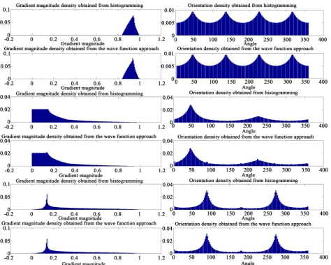
We would like to emphasize that our wave function method for computing the gradient density is very fast and straightforward to implement as it requires computation of a single Fourier transform. We ran multiple simulations on many different types of functions to assess the efficacy of our wave function me-thod. Below we show comparisons with the standard histogramming technique where the functions were sampled on a regular grid between

[

−0.125,0.125

] [

× −0.125,0.125

]

at a grid spacing of 13

1

2 . For the sake of convenience, we normalized the functions such that the maximum gradient magnitude value

(

∇S

)

_{is 1. Using the sampled values} Sˆ, we first computed the fast Fourier transform of exp_iS_τˆ_

  at τ =0.00004, then computed the power spectrum followed by normalization to obtain the joint gradient density. We also computed the discrete derivative of S at the grid locations to obtain the gradient ∇ =S

(

S Sˆ ˆx₁, x₂

)

and then determined the gradient density by histo-gramming. For better visualization, we marginalized the density along the radial and the orientation directions. The plots shown in Figure 1 provide visual, em-pirical evidence corroborating our theorem. Notice the near-perfect match be-tween the gradient densities computed via standard histogramming and our wave function method. The accuracy of the density marginalized along the orientations further strengthens our claim made in Section 1 about the wave function method serving as a reliable estimator for the histogram of oriented gradients (HOG). In Figure 2, we verify the convergence of our estimated den-sity to the true denden-sity as τ →0 _{in accordance with Theorem 3.2.}

6. Conclusions

Observe that the integrals

( )

_{( )}

( )

( )

_{( )}

( )

0 0

0 d , 0 d

I P I P

η η

τ u =

∫

_{ u} τ u u u =

∫

_{ u} u u

give the interval measures of the density functions Pτ and P respectively.

[image:17.595.64.539.71.451.2]

DOI: 10.4236/apm.2019.912051 1050 Advances in Pure Mathematics Figure 1. Comparison results. 1) Left: Gradient magnitude density, 2) Right: Gradient orientation density. In each sub-figure, we plot the density function obtained from histogramming and the wave function method at the top and bottom respectively.

spectrum of the wave function φ

( )

exp iS

( )

τ   =    

x

x . Hence we conclude that

the power spectrum of φ

( )

x can potentially serve as a jointdensityestimator

for the gradient of S at small values of τ _{, where the frequencies act as gradient} histogram bins. We also built an informal bridge between our wave function method and the characteristic function approach for estimating probability den-sities, by directly trying to recast the former expression into the latter. The diffi-culties faced in relating the two approaches reinforce the stationary phase me-thod as a powerful tool to formally prove Theorem 3.2. Our earlier result proved in [20], where we employ the stationary phase method to compute the gradient density of Euclidean distance functions in two dimensions, is now generalized in Theorem 3.2 which establishes a similar gradient density estimation result for arbitrary smooth functions in arbitrary finite dimensions.

[image:18.595.62.537.72.462.2]

DOI: 10.4236/apm.2019.912051 1051 Advances in Pure Mathematics Figure 2. Convergence of our wave function method as τ →0. The value of τ is steadily decreased from right to left, top to bottom.

estimated from a finite, discrete set of samples, instead of assuming that the function is fully described over a compact set Ω_{. In the future, we plan to} ex-tend this work and derive similar finitesampleerrorbounds for gradient density estimation in arbitrary higher dimensions.

Support

This research work benefited from the support of the AIRBUS Group Corporate Foundation Chair in Mathematics of Complex Systems established in ICTS-TIFR.

This research work benefited from the support of NSF IIS 1743050.

Conflicts of Interest

DOI: 10.4236/apm.2019.912051 1052 Advances in Pure Mathematics

References

[1] Parzen, E. (1962) On the Estimation of a Probability Density Function and the Mode. The Annals of Mathematical Statistics, 33, 1065-1076.

https://doi.org/10.1214/aoms/1177704472

[2] Rosenblatt, M. (1956) Remarks on Some Nonparametric Estimates of a Density Function. The Annals of Mathematical Statistics, 33, 832-837.

https://doi.org/10.1214/aoms/1177728190

[3] Silverman, B.W. (1986) Density Estimation for Statistics and Data Analysis. Chap-man and Hall/CRC, New York.https://doi.org/10.1007/978-1-4899-3324-9

[4] Bishop, C.M. (2006) Pattern Recognition and Machine Learning (Information Science and Statistics). Springer, New York.

[5] Jones, D.S. and Kline, M. (1958) Asymptotic Expansions of Multiple Integrals and the Method of Stationary Phase. Journal of Mathematical Physics, 37, 1-28.

https://doi.org/10.1002/sapm19583711

[6] Cooke, J.C. (1982) Stationary Phase in Two Dimensions. IMA Journal of Applied Mathematics, 29, 25-37.https://doi.org/10.1093/imamat/29.1.25

[7] McClure, J.P. and Wong, R. (1991) Two-Dimensional Stationary Phase Approxima-tion: Stationary Point at a Corner. SIAM Journal on Mathematical Analysis, 22, 500-523.https://doi.org/10.1137/0522032

[8] McClure, J.P. and Wong, R. (1997) Justification of the Stationary Phase Approxi-mation in Time-Domain Asymptotics. Proceedings: Mathematical, Physical and Engineering Sciences, 453, 1019-1031.https://doi.org/10.1098/rspa.1997.0057

[9] Wong, R. (1989) Asymptotic Approximations of Integrals. Academic Press, New York.

[10] Wong, R. and McClure, J.P. (1981) On a Method of Asymptotic Evaluation of Mul-tiple Integrals. Mathematics of Computation, 37, 509-521.

https://doi.org/10.2307/2007443

[11] Dalal, N. and Triggs, B. (2005) Histograms of Oriented Gradients for Human De-tection. IEEE Conference on Computer Vision and Pattern Recognition, 20-26 June 2005, San Diego, 886-893. https://doi.org/10.1109/CVPR.2005.177

[12] Zhu, Q., Yeh, M.-C., Cheng, K.-T. and Avidan, S. (2006) Fast Human Detection Using a Cascade of Histograms of Oriented Gradients. IEEE Conference on Com-puter Vision and Pattern Recognition, New York, 17-22 June 2006, 1491-1498.

https://doi.org/10.1109/CVPR.2006.119

[13] Suard, F., Rakotomamonjy, A. and Bensrhair, A. (2006) Pedestrian Detection Using Infrared Images and Histograms of Oriented Gradients. IEEE Conference on Intel-ligent Vehicles, Tokyo, 13-15 June 2006, 206-212.

https://doi.org/10.1109/IVS.2006.1689629

[14] Bertozzi, M., Broggi, A., Del Rose, M., Felisa, M., Rakotomamonjy, A. and Suard, F. (2007) A Pedestrian Detector Using Histograms of Oriented Gradients and a Sup-port Vector Machine Classifier. IEEE Conference on Intelligent Transportation Systems, Seattle, 30 September-3 October 2007, 143-148.

https://doi.org/10.1109/ITSC.2007.4357692

[15] Vapnik, V.N. (1998) Statistical Learning Theory. Wiley-Interscience, New York. [16] Hu, R. and Collomosse, J. (2013) A Performance Evaluation of Gradient Field HOG

DOI: 10.4236/apm.2019.912051 1053 Advances in Pure Mathematics

[17] Arute, F., Arya, K., Babbush, R., Bacon, D., Bardin, J.C., Barends, R., Biswas, R., Boixo, S., Brandao, F., Buell, D.A., et al. (2019) Quantum Supremacy Using a Pro-grammable Superconducting Processor. Nature, 574, 505-510.

https://doi.org/10.1038/s41586-019-1666-5

[18] Boixo, S., Isakov, S.V., Smelyanskiy, V.N., Babbush, R., Ding, N., Jiang, Z., Bremner, M.J., Martinis, J.M. and Neven, H. (2018) Characterizing Quantum Supremacy in Near-Term Devices. Nature Physics, 14, 595-600.

https://doi.org/10.1038/s41567-018-0124-x

[19] Markov, I.G., Fatima, A., Isakov, S.V. and Boixo, S. (2018) Quantum Supremacy Is Both Closer and Farther than It Appears.arXiv:1807.10749 [quant-ph]

[20] Gurumoorthy, K.S. and Rangarajan, A. (2012) Distance Transform Gradient Densi-ty Estimation Using the Stationary Phase Approximation. SIAM Journal on Ma-thematical Analysis, 44, 4250-4273.https://doi.org/10.1137/110859336

[21] Bracewell, R.N. (1999) The Fourier Transform and Its Applications. 3rd Edition, McGraw-Hill, New York.

[22] Fukunaga, K. and Hostetler, L. (1975) The Estimation of the Gradient of a Density Function with Applications in Pattern Recognition. IEEE Transactions on Informa-tion Theory, 21, 32-40.https://doi.org/10.1109/TIT.1975.1055330

[23] Gurumoorthy, K.S. and Rangarajan, A. (2014) Error Bounds for Gradient Density Estimation Computed from a Finite Sample Set Using the Method of Stationary Phase. arXiv:1404.1147 [stat.CO]

[24] Scott, D. (1979) On Optimal and Data-Based Histograms. Biometrika, 66, 605-610.

https://doi.org/10.1093/biomet/66.3.605

[25] Cencov, N.N. (1962) Estimation of an Unknown Distribution Density from Obser-vations. Soviet Mathematics, 3, 1559-1562.

[26] Wahba, G. (1975) Optimal Convergence Properties of Variable Knot, Kernel, and Orthogonal Series Methods for Density Estimation. Annals of Statistics, 3, 15-29.

https://doi.org/10.1214/aos/1176342997

[27] Griffiths, D.J. (2005) Introduction to Quantum Mechanics. 2nd Edition, Prentice Hall, Upper Saddle River.

[28] Feynman, R.P. and Hibbs, A.R. (2010) Quantum Mechanics and Path Integrals: Emended Edition. Dover Books on Physics. Dover, Mineola.

[29] Goldstein, H., Poole, C.P. and Safko, J.L. (2001) Classical Mechanics. 3rd Edition, Addison Wesley, Boston.https://doi.org/10.1119/1.1484149

[30] Billingsley, P. (1995) Probability and Measure. 3rd Edition, Wiley-Interscience, New York.

DOI: 10.4236/apm.2019.912051 1054 Advances in Pure Mathematics

Appendix A. Proof of Lemmas

1) Proof of Finiteness Lemma

Proof. We prove the result by contradiction. Observe that u is a subset of the compact set Ω_{. If} _u is not finite, then by Theorem (2.37) in [31], u has a limit point x0∈ Ω. If x0∈ ∂Ω, then u∈ giving a contradiction.

Otherwise, consider a sequence

{ }

x_{n n}∞=₁, with each xn∈u, converging to x0.

Since ∇S

( )

xn =u for all n, from continuity it follows that ∇S

( )

x0 =u and

hence x0∈u. Let pn ≡xn−x0 and n n n

≡ p h

p . Then

( )

( )

0 ₀

lim n n ,

n

n

S S

→∞

∇ − ∇ −

=0

x

x x p

p



where the linear operator x₀ is the Hessian of S at x0 (obtained from the

set of derivatives of the vector field _∇S:_d _→d _{at the location}

0

x ). As

( )

n

( )

0

S S

∇ x = ∇ x =u and x₀ is linear, we get

0

lim n .

n→∞x h =0

Since hn is defined above to be a unit vector, it follows that x0 is rank

defi-cient and det

( )

_x0 =0. Hence x0∈ and u∈ resulting in a

contradic-tion.

2) Proof of Neighborhood Lemma

Proof. Observe that the set  defined in (2.2) is closed because if x0 is a

limit point of , from the continuity of the determinant function we have

( )

0

det _x =0 and hence x0∈. Being a bounded subset of Ω,  is also

compact. As ∂Ω _{is also compact and} ∇S _{is continuous,}  is compact and hence _d_{− is open. Then for}

0∉

u , there exists an open neighborhood

( )

0

r u

 for some r>0 _around u₀ such that r

( )

u0 = ∅. By letting

2 r

η = _{, we get the required closed neighborhood} _η

( )

u₀ ⊂_r

( )

u₀ contain-ing u0.

Since det

( )

_x ≠ ∀ ∈0, x _u0, points 1, 2 and 3 of this lemma follow directly from the inverse function theorem. As u0 is finite by Lemma 2.1, the closed

neighborhood η

( )

u0 can be chosen independently of x∈u0 so that

points 1 and 3 are satisfied ∀ ∈x _u0. In order to prove point 4, note that the eigenvalues of x are all non-zero and vary continuously for x∈η

( )

x . As

the eigenvalues never cross zero, they retain their sign and so the signature of the Hessian stays fixed.

3) Proof of Density Lemma

Proof. Since the random variable X is assumed to have a uniform distribution on Ω_{, its density at every location} x∈ Ω equals _µ

_{( )}

1_Ω . Recall that the