Formation of stellar clusters

Formation of stellar clusters

Romas Smilgys,

1

?

_{Ian A. Bonnell}

1

1_{Scottish Universities Physics Alliance (SUPA), School of Physics and Astronomy, University of St. Andrews, North Haugh, St. Andrews, Fife KY16 9SS, UK}

Accepted XXX. Received YYY; in original form ZZZ

ABSTRACT

We investigate the triggering of star formation and the formation of stellar clusters in molecular clouds that form as the ISM passes through spiral shocks. The spiral shock com-presses gas into∼100 pc long main star formation ridge, where clusters forming every 5-10

pc along the merger ridge. We use a gravitational potential based cluster finding algorithm, which extracts individual clusters, calculates their physical properties and traces cluster evo-lution over multiple time steps. Final cluster masses at the end of simulation range between 1000 and 30000 Mwith their characteristic half-mass radii between 0.1 pc and 2 pc. These

clusters form by gathering material from 1020 pc size scales. Clusters also show a mass -specific angular momentum relation, where more massive clusters have larger -specific angular momentum due to the larger size scales, and hence angular momentum from which they gather their mass. The evolution shows that more massive clusters experiences hierarchical merging process, which increases stellar age spreads up to 2-3 Myr. Less massive clusters appear to grow by gathering nearby recently formed sinks, while more massive clusters with their large global gravitational potentials are increasing their mass growth from gas accretion.

Key words: stars: formation – stars: luminosity function, mass function – globular clusters

and associations: general, interstellar medium, galaxies: star formation.

1 INTRODUCTION

Star formation is one of the most important processes in galactic evolution, transforming gas into stars and providing the visible out-put as well as the chemical and energetic feedback into the galaxy. Current understanding is that at least half of all stars, and potentially all massive stars, form in stellar clusters (Lada & Lada 2003;de Wit et al. 2004;Zinnecker & Yorke 2007;Bressert et al. 2010;Oh et al.

2015;Megeath et al. 2016;Stephens et al. 2017). Understanding

how stellar clusters form is on ongoing challenge with many ob-servational studies trying to determine the exact initial conditions (Kauffmann & Pillai 2010;Cyganowski et al. 2017;Csengeri et al. 2017). Models for cluster formation show that a turbulent molecular clump that is gravitationally unstable fragments hierarchically into small clusters which eventually merge to form larger stellar systems (Bonnell et al. 2003,Bate et al. 2003,Krumholz & Bonnell 2007,

Offner et al. 2008,Smith et al. 2009). Observations of star

forma-tion in infrared dark clouds such asPeretto et al.(2013) shows the fragmentation of the filamentary structure (André et al. 2014,Hacar et al. 2017) feeding into the formation of a stellar cluster.

Numerical simulations have provided significant insight into the dynamical nature of star formation (Bate et al. 2003;Bonnell et al. 2003;Bonnell et al. 2011;Bertelli Motta et al. 2016), show-ing the importance of turbulence, collapse, fragmentation, interac-tions and accretion. Although useful in highlighting the physical

? _{E-mail: [email protected]}

processes, these numerical simulations suffer from their overly-idealised initial conditions. Our (Bonnell et al. 2011) study showed that a small variation in gravitational boundedness along a cloud results in significantly different stellar populations, clusterings, star formation rates, efficiencies, and stellar IMFs. Initial conditions have a major impact on all star formation properties, and hence using self-consistent initial conditions is crucial to develop realistic models.

Recent simulation work, likeBate et al.(2003),Bonnell et al.

(2003),Bonnell et al.(2011),Krumholz et al.(2011) gives results for individual molecular clouds and forming clusters. Observations such as those ofRathborne et al.(2015) support the concept that clusters grow hierarchically. However, observations are limited in terms of 3D spatial information and time evolution. Real molecular clouds in spiral galaxies (Elmegreen 2007) appear as high density regions in the ISM during the passage through the spiral arms. Works likeDobbs et al.(2006),Dobbs et al.(2012),Bonnell et al.

(2013) were first attempts to set up more realistic initial conditions in simulations, which could have large effects on how clouds are shaped and how star clusters are forming.

There are large numbers of observations being made which contribute towards understanding the processes of stellar cluster formation. Observations are necessarily wide ranging, covering the mass-radius relation (Marks & Kroupa 2012;Pfalzner et al. 2016;

Csengeri et al. 2017), stellar age spreads (Getman et al. 2014,Kuhn

et al. 2015b), line of sight kinematics (Fűrész et al. 2008,Hacar

2

R. Smilgys & I. A. Bonnell

Gutermuth et al. 2009), spatial structure (Kuhn et al. 2014,Kuhn

et al. 2015a,Kuhn et al. 2015b). However, very few properties can

be compared directly between simulations and observations. Sim-ulations are limited by initial conditions and the physics included, while observations are limited by 2D projection in the sky as well as their inability to show us the the past or future evolution of clusters. Star formation is also likely to be affected by feedback from the stars, especially young high mass stars. Feedback may also help to explain the low efficiencies of star formation seen on different scales (e.g.Megeath et al. 2016;Dubois & Teyssier 2008;Ostriker & Shetty 2011;Girichidis et al. 2016;Gatto et al. 2017), but low efficiencies are also possible in the absence of feedback (Bonnell

et al. 2011;Louvet et al. 2014). Simulations of star formation

in-cluding feedback generally result in a significant (factor 2) decrease in the star formation efficiencies (e.g.Dale & Bonnell 2012;Dale

et al. 2014,2015;MacLachlan et al. 2015;Dale 2017). Although

feedback can decrease the efficiency of star formation, it does not in general stop ongoing star formation. Instead, the feedback finds weak points (lower density) in the surrounding gas through which it can be channelled and escape the dense clump.

Gas removal can affect the overall dynamics and lifetimes of forming clusters if it contributes a dominant proportion of the clus-ter mass. Several N-body studies have investigated the effect of gas removal in young stellar clusters via an assumed potential. These studies, although not fully consistent in terms of the effect of feed-back on gas, provide valuable insight into the potential cluster evo-lution (Kroupa et al. 2001;Marks & Kroupa 2012;Brinkmann et al. 2017;Banerjee & Kroupa 2017). For example,Banerjee & Kroupa

(2015) showed that gas and dissipation free hierarchical mergers have difficulty producing large smooth clusters and that systems, such as R136, NGC3603 and the ONC could have formed from monolithic collapse scenario. However, in these works gas was re-placed by static potential, neglecting the dissipational properties of gas dynamics which can greatly decrease the merger timescale (Bonnell et al. 2011). Indeed, several observational studies find ev-idence for hierarchical mergers in terms of kinematical subgroups in young stellar clusters (Sabbi et al. 2012.).

R136, NGC3603 and the ONC cases does not necessarily con-firm if these clusters has formed from monolithic collapse or internal structure, produced by mergers has been smoothed out by the in-teraction with gas. In contrast, observational studies find evidence of the highly fragmented nature of cluster formation (Beuther et al.

2015; Csengeri et al. 2017; Zhang et al. 2009), for kinematical

subgroups in young stellar clusters (Sabbi et al. 2012) and of clus-ters that appear in close proximity such that a subsequent merger is possible, pointing to scenarios where hierarchical mergers are a likely process in star cluster formation (Bonnell et al. 2003;Walker

et al. 2015). These observational evidences brings support to cluster

formation through merging scenario, which we will investigate in details in this work.

2 METHODS

2.1 SPH simulations

In a previous work we analysed triggering of star formation during the spiral arm passage Smilgys & Bonnell(2016). Here we use the simulation data ofBonnell et al.(2013) which uses assumed spiral potential from Dobbs et al.(2006) through which ISM is allowed to flow. We determine physical cluster properties, such as masses, densities, sizes, binding energies and their evolution over

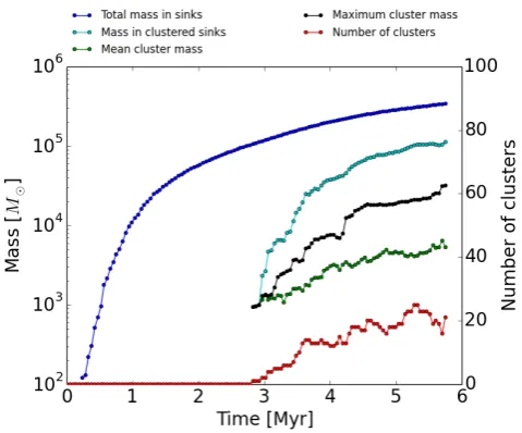
Figure 1.The sink and cluster statistics are plotted over the simulation. Star formation, modelled by sink particles, starts early (0.5 Myr), but clusters appear only from 3 Myr. The number of clusters is shown on right hand side axis. The mass in sinks and in clusters is also plotted (scale at left), showing continuous star formation throughout the simulation.

time. These key parameters allow us to investigate stellar cluster formation mechanisms and dynamics free from the intrinsic as-sumptions due to the idealised initial conditions.

Bonnell et al.(2013) simulation was constructed from a set

of nested simulations starting from a full Galactic disc simulation over 350 Myr, with a 50 Myr high-resolution counterpart focusing on the formation of dense clouds in the spiral arms, and a final simulation to follow star formation over 5.8 Myr. The final stage, which we analyse here, included self-gravity and modelled a 250 pc region containing 1.9×106 M mass. This simulation used 1.29×107 SPH particles with 0.15 M masses. Star formation is followed through the use of sink particles (Bate et al. 1995). A minimum mass for the sink particles corresponds to≈70 SPH

particles representing one SPH kernel, or≈ 11 M with a sink radius of 0.25 pc to accrete bound, infalling gas particles while all particles penetrating within 0.1pc were accreted. The sink particles therefore do not represent individual stars but rather a small cluster of stars or star forming region. Gravitational interactions between sinks were smoothed within 0.025 pc.

Simulations used for our work, do not have any stellar feedback or magnetic fields, and is hence designed to investigate how stel-lar clusters are forming in more realistic initial conditions, which includes spiral arm dynamics. We also point out here that before including feedback and magnetic fields, it is essential to understand what properties of forming clusters are being defined purely by the spiral arm dynamics. Stellar feedback could be more relevant for later stages of simulation, once massive stars form, while at early stages only magnetic fields can slow down the formation of the first stars.

2.2 Cluster definition

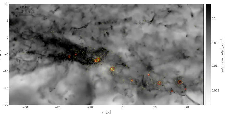
Figure 2.A side-on view through main star forming region in Galactic spiral arm is shown at at the end of the simulation. The LOS here is pointing through the Galactic plane, along y direction. The z direction is perpendicular to Galactic plane, where z=0 pc is the Galactic equator plane. The figure shows greyscale column density map for gas, the distribution of recently formed stars (in terms of sink particles) as yellow dots, and the positions of stellar clusters as red open circles. The map shows that dense gas clouds and forming clusters do not necessarily lie in Galactic mid-plane.

Figure 3.A side-on view through the main star forming region in the Galactic spiral arm is shown at at the end of simulation. The figure shows sink particles colour-coded by their stellar age. We see a clear age gradient from left to right which coincides with a decrease in the column density of gas in the same direction. This is evidence of a sequential star formation process triggered by the passage of the ISM through the spiral shock.

For SPH simulations data, the cluster finding algorithm has to find clusters based on sink particle positions and masses. There are two steps to follow in order to obtain a robust cluster definition and to follow cluster formation history: static cluster definition at a given time and dynamical cluster definition by linking the same cluster from one time step to another.

Our cluster definition is based on sink local and enclosed grav-itational potentials. Firstly each sink has assigned its local potential from surrounding neighbour sinks within 2 pc. The list of all sinks at a given time step is sorted by these potentials and the deepest po-tential sink is picked as a starting point. This first and lowest local potential sink is set as a centre of the cluster and enclosed potentials are calculated on all sinks within 2 pc around it. Next sinks are continuously added to the most bound cluster if their local potential is not deeper than twice that of the enclosed potential of the cluster. If no such cluster is found and the sink has its local potential depth

below the upper potential threshold (−1011cm2s−2), it starts a new

cluster. The search is finished when it reaches the first sink with its local potential above the background level. Clusters, which have fewer than six members are removed after the search is completed. Using the enclosed potential to build clusters results in a bias to-wards the selection of spherical rather than filamentary structures. We use−1011cm2s−2 potential threshold, as systems below this

4

R. Smilgys & I. A. Bonnell

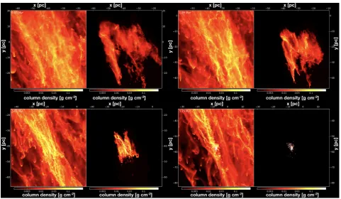
Figure 4.The face-on view evolution of the most massive cluster forming region calculated at four different times. The left hand panel in each pair shows column density of all gas in the region, while the right hand panel shows only gas accreted by the cluster. Maps show the compression of the ISM by the spiral shock passes. The central highest density region becomes gravitationally bound and forms a∼30000 Mcluster.

We repeat the cluster finding process throughout the entire duration of the simulation at each time step. Clusters can be traced over time by linking two clusters between two neighbouring time steps. A cluster is assumed to be the same if particles representing more than 50% of the cluster mass from the current time steptiare

found in it at the next time stepti+1. Clusters can also merge. If

the mass of the smaller cluster is larger than 30% of the total mass of both parts, then these clusters are major mergers (otherwise they are minor mergers). Mergers can be traced by searching if most of the sinks from two separate clusters at timetiare found in a single

cluster at the next time stepti+1. Linking clusters over all time steps

allows us to create a merger tree for the clusters.

In order to remove fluctuations that occur when a cluster is near the cluster definition boundary, we smooth the cluster finding algorithm over neighbouring time steps. Cluster lifetimes are cal-culated along the merger tree branch. If the lifetime is only 1 time step, clusters are checked to ensure they do not merge again into the same cluster - if so, sinks from the temporary cluster are re-assigned to the main cluster.

3 RESULTS

We make use of theBonnell et al.(2013) self-gravity simulation that inherited its initial conditions from a large scale Galaxy simulation. It contains∼12 million SPH particles. The inherited initial

condi-tions set the galactic scale shock, and compresses the ISM to higher densities to start star formation. The gas motions into the shock are predominantly along y-axis of the simulation. Star formation takes place continuously as the shock travels through the gas, forming 2000 sinks and around 20 clusters by the end of the simulation. In

addition, the shock reaches one side slightly earlier than another, and thus creates a gradient in stellar ages along the spiral arm.

3.1 Cluster statistics

We apply our cluster finding algorithm to the entireBonnell et al.

(2013) self-gravity simulation in order to find clusters of sinks. Clustering statistics based on the gravitational potential definition are shown in Figure1. From the figure we see that at the beginning of the simulation there are no sinks and no clusters. The first sinks form quite early, in the first Myr of the simulation. However, clusters appears only around 3 Myr. This show that the first sinks form individually in the highest density fast collapsing clumps. Clusters appear slightly later when at least 6 sinks assemble in a compact region and meets the definition. Figure1shows that star formation is continuously occurring in the simulation, with individual sinks, and clusters growing in mass, and in numbers throughout the simulation. The number of clusters appears to be growing up to∼20 at the end

of simulation. From∼4 Myr fluctuations appear in the number of

clusters, indicating that clusters also undergo mergers which add to their growth rates but decrease the total numbers of clusters present.

3.2 Cluster forming regions

reached that side slightly earlier and triggered star formation there. As the spiral shock passed through, part of the gas was consumed by star formation, while another part moved with the shock or even started to expand as post-shock leaves the region. We can see very high column densities in the Figure2between−30 [pc]<x<−10

[pc], where the shock is moving through the gas. There is very little star formation in this part. However, looking at Figure3we can see that star formation here only starts to happen with visible several very young (< 0.5 Myr) clusters (around [−15;−5]), which

may merge in the future and form another big cluster there. Figures

2 and 3gives a support towards both sequential (Elmegreen &

Lada 1977) and triggered star formation models: the sequential star

formation appears as the spiral shock continuously propagates to the left but at the same time individual clouds are compressed, where star formation is triggered.

Most of the high density star forming regions in Figure2are visible 5-15 pc below the Galactic plane. This is due to the larger scale dynamics that drive the star formation (Bonnell et al. 2013), where spiral shocks and cloud-cloud collisions can cause some star forming regions to be significantly out of the plane of the Galaxy.

Right hand side panel of Figure3shows zoomed in region onto two most massive final clusters. Cluster at left shows some younger stars in the core, but also a few older ones. Stars near the outside are mostly older. Cluster at right shows younger stars in the outer regions, some younger in core but overall a bit older.

We take the most massive cluster at the end of the simulation, which is visible on the edge of high density clouds in the middle of Figure2, and trace all its environment, accreted gas and sinks backwards in time. By finding sinks which belong to the cluster, we are also mapping all the gas particles that ultimately contributed to form the cluster. As all accreted particles are found, the cluster mass is assumed to be conserved over all time steps and the centre of mass of the system is well defined. We follow this cluster mass centre to illustrate the formation of the cluster in x-y position maps at four different time steps. Figure4shows the evolution of the gas and sinks forming the most massive cluster, plotted in the cluster’s centre of mass frame. Each of 4 panels has a map of surface density derived from all gas particles in the region (left) and a map of surface density calculated from not yet accreted gas particles that contribute mass to the final cluster (right).

Initial gas cloud with the size of∼40 pc is contracting down

to several pc size cluster, a contraction of > 10 times over 6 Myr. Comparison between left and right hand side panels show that ac-creted cluster gas are embedded all the time in the largest density areas of the region. Accreted gas distribution (right panels) well matches the distribution of all gas (left panels). However, most of the particles visible in the left hand panel are not accreted by any sinks and so do not play a part in forming the cluster. Gas particles accreted by sinks not belonging to the cluster are excluded (right panels). The internal geometry of the region is highly fragmented with visible clumps (where the first sinks form) and filaments. Even if the cloud collapses as the whole, the internal structure of clumps and filaments keeps changing over the time. The presence of the galactic spiral shock is visible in the left hand panels, as the shock compresses widely distributed clouds to form a thin ridge through 6 Myr, extending from the top left to bottom right side of the map. Figure5shows the initial regions from which the various clus-ters form and accrete their final mass. These gas particles are shown in Figure5as coloured particles, with the colour representing the mass of the final cluster. The grey particles in Figure5show the non cluster-forming gas. We note that cluster forming gas clouds are initially embedded in higher density regions. The highest mass

Figure 5.The face-on view of the main star forming region showing the initial size scales of the star forming clouds. Individual cluster forming reservoirs are colour coded by final cluster mass and plotted on the top of a greyscale map of all gas in the region. The map shows that clouds are aligned to the main ridge and that mass is coming into clusters from 10-30 pc size regions.

Figure 6.This diagram shows the location of star formation and subsequent accretion of gas particles during the cluster formation process.

clusters form from the central high density region, and there are small mass clusters forming outside this region. We also notice the trend that more massive clusters form from larger clouds. The spiral shock is coming from the bottom-right side of the diagram and there are visible trails of particles, which are coming with the shock to the main star forming region and are also accreted by sinks in clusters (purple trails in the bottom side of the diagram). As the material is incoming with the small pitch angle to the spiral arm, the section of low density inter-arm gas can be seen in the bottom-left side of the diagram.

3.3 Accretion histories

6

R. Smilgys & I. A. Bonnell

accretion histories for the two most massive clusters are shown in Figure6. Most massive cluster is visible slightly to the right from the centre of the picture, while the second most massive cluster -slightly left and down. Particle positions are plotted relative to the centre of mass frame of all clusters in the simulation. Accreted gas particles are plotted at their final locations, and colour-coded with the time of their accretion. Sink forming locations are plotted as purple dots. Sink movement paths are shown as grey lines.

This figure shows the formation process of the two clusters. The first sinks are forming in relatively isolated regions. They form along filaments, and then flow down the filaments. Additional sink formation forms small clusters which grow through accretion, and mergers. Star formation continues along the filament and down to the intersection points where the filaments flows, and accompanying clusters merge to form the final cluster.

4 CLUSTER PROPERTIES

In the following sections, we analyse the developing properties of the stellar clusters in our simulation. It should be noted that as the simulations do not include feedback, the properties could be affected (Parker & Dale 2013;Banerjee & Kroupa 2015).Parker & Dale(2013) usesDale et al.(2012,2013) simulations to show that clusters formed with feedback have only slighlty smaller masses, bigger sizes and larger dynamical times.

4.1 Mass merger tree

We trace clusters between multiple time steps in order to follow the evolution of cluster properties over their formation histories. The simplest cluster property is its mass. As we know which sinks are members of which cluster, we obtain cluster masses over mul-tiple time steps. Mulmul-tiple cluster events can occur over time, such as creation, dissolution, merging and splitting. As our simulation is targeting cluster formation process, we naturally have merging processes of two clusters occurring at particular time steps. Plotting the cluster masses over time produces a mass-merger tree diagram (Figure7). The intersection points show major merger events as red, if the child cluster’s mass exceeds 30% of the parent’s cluster mass. Minor merger events occur when the child’s mass is below 30% of the parent cluster’s mass and are plotted as blue points. Colours show the total lifetime of the cluster, from its formation until it merges with the parent cluster.

Firstly we notice that cluster mass growth and merging con-tinues throughout the simulation. Clusters continue to grow as long as there is surrounding gas, sinks or smaller clusters to be accreted into larger central clusters. Merger events occur most frequently for larger mass clusters, while low mass systems have small numbers of mergers in their histories. Cluster merging also appears to be a channel of significant mass growth over the time for the more massive systems. Large final mass clusters have also much longer merging histories, well traced over∼2.5 Myr, while small clusters

have lifetimes of only 0.5 - 1 Myr.

4.2 Mass-radius relation

One of the properties of our simulated clusters is their mass-radius relation. This must reflect the formation process in some way and thus should form a good property with which to compare to real clusters. As cluster definition returns a list of cluster members, the

characteristic cluster sizes can be determined. We use twice the half-mass radius in order to characterise full cluster sizes. The half-half-mass radius for each cluster is found by sorting cluster member sinks by their distances from the cluster’s centre of mass. We then use cumulative enclosed mass radial profiles to find at what radius half of the cluster mass is enclosed. We plot twice the half-mass radius as a robust measure of the effective size of the cluster that does not suffer from the variation in position or classification of the outermost cluster members. When cluster masses and sizes are determined we get a cluster mass-radius relation. We then plot cluster mass-radius relation over all clusters at two time steps - blue for early times (5 clusters) and red for late times (16 clusters) (Figure8).

The diagram shows that more massive clusters also have larger half-mass radii. Low mass clusters, taken to be those with<1000 Mhave half-mass radii of 0.1 pc. On the other hand high mass clus-ters have half-mass radii of 0.5 - 2 pc. We found clusclus-ters between the -1011_cm2_s−_{2iso-potential line and 100 Mpc}−_{3iso-density line.} On one hand this looks as artificial disadvantage of the definition, as clusters are more likely to be traced as spherical systems. But on the other hand these spherical and centrally condensed systems are virialized and do not change their geometrical shape rapidly in time.

Several physical processes are important for the mass-radius relation. These include the gravitational collapse that forms the clus-ter, subsequent merger events and ongoing gas and sink accretion. Gravitational collapse causes the size of the system to decrease. On the other hand, mergers grow the cluster mass but there is also an increase in the combined cluster size.

Blue solid line shows mass radius relation from fitting obser-vational data of star forming clumps byUrquhart et al.(2014). The line appears to be slightly above our data points. This could be becauseUrquhart et al.(2014) mass-radius relation was fitted for clumps, which are still collapsing. If clumps would continue to col-lapse towards clusters, their radii would decrease and could match our simulated clusters.

We also plot a black solid line in Figure8which showsMarks & Kroupa(2012) theoretically predicted birth mass-radius relation, obtained by using binary populations in clusters.Marks & Kroupa

(2012) mass-radius relation is derived for the densest collapse state of the bulk young stellar population in the cluster, and how these limit the binary statistics. This indirect measurement of the mass-radius relationship is powerful but inherently makes assumptions as to the natal binary properties. Subsequent dynamics and tidal evolution will likely affect the cluster properties (Moeckel et al. 2012).

4.3 Cluster angular momentum

Figure 7.The diagram showing the mass-merger tree of clusters. The diagram shows major (smaller cluster has more than 30% of total cluster mass after merging) and minor merging events. More massive clusters also have longer lifetimes and more extended merging histories.

Figure 8.The cluster mass-radius relation is shown at two different times of the simulation. The plots shows how the size of the clusters increases with the mass of the cluster, with an approximate Rh al f ∼Mγ_{c l u s t} relation, whereγis about 1.

4.4 Mass growth of stellar clusters

Accretion of stars (Pflamm-Altenburg & Kroupa 2007) and gas

(Pflamm-Altenburg & Kroupa 2009) from the environment has

been investigated in pre-existing clusters. Here we address what contributes mostly in forming different mass clusters - accretion of stars or gas. In order to measure the accretion of gas into the cluster, we follow the change of mass of the sinks that are already in the cluster. In Figure10, we plot this as a fraction of the cluster mass and as a function of the total cluster mass.

The first thing we notice is that clusters with low masses appear to have only a small fraction of their mass being due to gas accretion. This is partially by definition in that the cluster first "forms" when

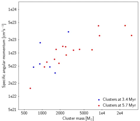
Figure 9.The stellar clusters’ specific angular momentum is plotted as a function of cluster mass. Higher mass clusters have larger specific angular momenta, indicating that rotation, due to accreting mass from further away, is more important in such clusters.

six or more sinks are sufficiently close, and hence have a minimum mass to which gas accretion does not contribute. Nevertheless, we see that the fraction of the total mass contributed by gas accretion increases with cluster mass. At high cluster masses, direct accretion of gas is seen to contribute nearly half the total mass of the system. Secondly, we notice that mass gain from gas accretion inside clusters is always less than 40 - 50 % of the total cluster mass (This neglects the gas accretion onto the initial cluster formation consisting of a minimum of several hundred solar masses). The diagram clearly shows that gas accretion on clustered sinks has contributed mostly for large mass clusters.

8

R. Smilgys & I. A. Bonnell

Figure 10.The growth in clusters’ mass due to accretion of gas inside the cluster. Gas accretion is an increasingly important contributor to cluster masses as a function of mass. This is due to the larger range from which they can accrete due to their deeper gravitational potential.

Figure 11.The accretion timeline is shown for the three most massive clusters. Sink formation and accretion extend over several Myr as the clusters form from star formation that extends more than 10 pc from the centre of mass. Some of 9000 Mcluster sinks form as far as 18 - 20 pc away at very early 0.5 Myr simulation time, and comes into the cluster later.

gas accretion on its existing sinks, then it moves upwards to larger accreted gas mass over cluster mass ratios and also larger cluster masses. This is visible as a forest of parallel trails going upwards in Figure10for low mass clusters at 2-4 Myr. If cluster accretes sinks or other clusters, they "jump" downwards, which is visible for larger clusters at later times (4-6 Myr).

Figure 12.Clusters’ mean stellar ages are plotted as functions of cluster mass and time in the simulation. The Mean ages change only slowly as long as star formation and accretion are ongoing. Once star formation ceases, the clusters appear to age normally, at near constant mass. The only mass growth is then limited to the merger of other clusters.

Figure 13.Cluster stellar age dispersion is plotted as a function of cluster mass and time. Low mass young clusters show low stellar age dispersion while large mass clusters have rich merging histories, resulting in larger stellar age dispersion.

4.5 Cluster age spreads

The merging process leads not only to a growth in mass, but also to a naturally larger age spread as the resultant clusters are formed by mixing different systems formed in different environments. Figure

11shows the accretion histories, in terms of accretion time versus the radius at which particle has been accreted. Here we plot only three most massive final clusters and trace their sinks backwards in time to where they formed. The common centre of mass for the system is calculated from all particles which make up the final mass of the cluster.

indi-cating continuous cluster collapse. We see that the cluster collapse is continuous over all time steps as sinks are continuously moving towards smaller radii. We also see that accretion takes place over several Myrs, in the absence of feedback. While feedback is often assumed to halt ongoing star formation, simulations show that star formation can continue due to the channelling of feedback away from the dense star forming gas (Dale & Bonnell 2012;Dale et al.

2014, 2015;Dale 2017). The large dispersion in accretion times

of various sinks originating in different regions produces signifi-cant spreads in stellar age in the final clusters. Smaller sub-clusters, which are visible as groups of paths, have smaller age dispersions. On the other hand, smaller clusters, which have yet to merge, display smaller age dispersions.

In Figure 12 we plot mean stellar ages for each cluster as a function of cluster mass and time. Stellar ages for each sink are calculated as a mass weighted average of accretion times for already accreted gas particles. This gives, for each sink, its stellar age, which can be different from the time since the sink first formed. The stellar age is smaller than sink age due to more recent accretion events. As we do not fully resolve star formation, we cannot distinguish whether this ongoing accretion could be forming additional stars, or accreting into pre-existing stars. Ongoing accretion onto young stars can also significantly reduce their apparent ages (Tout et al. 1999). We noticed that in our simulation stellar ages are on average 2/3 that of sink ages. Finally the cluster mean stellar age is just an average of stellar ages for all its members. Figure12show the visible trails of individual clusters over different times. At early times, sinks in clusters are accreting intensively and thus, their mean stellar ages increase slowly.

Once accretion in the cluster stops (as occurs when most ma-terial is accreted), the mean stellar age starts to increase rapidly and cluster mass growth slows down. During this phase, the tracks can be seen to be almost vertical in Figure12. There is also a visi-ble trend with mean stellar ages for early times slightly increasing for higher mass clusters. Stellar age dispersion similarly increases for more massive clusters, as they have experienced more mergers, bringing together stars which have formed at different times in a wider variety of environments.

We also show stellar age dispersions in Figure13, which are calculated as an age dispersion of all accretion events over all cluster members. The diagram shows a clear trend that stellar age dispersion increases for higher mass clusters. This is in a good agreement with merging scenario, as more massive clusters have experienced more mergers, bringing together stars of different ages from a wider variety of environments.

5 CONCLUSIONS

We performed an in depth analysis of how stellar clusters form in large Galactic scale simulations that resolve individual cluster form-ing regions, but neglect feedback processes. Galactic spiral shocks assemble clouds in the ridge-like structures, where we measured a stellar age gradient as the shock approaches one side of the ridge earlier than another. Older clusters are found in the regions that entered the spiral shock earlier. Younger clusters, and ongoing star formation, are associated with regions that more recently entered the spiral shock and hence are also associated with dense gas clouds. Our analysis relies on a physically based cluster definition, which uses local and enclosed gravitational potentials in order to separate individual clusters. We noticed that a robust physical cluster

definition can be one of the most vital steps before determining further physical properties and relations for stellar clusters.

The Lagrangian nature of SPH allowed us to trace individ-ual cluster formation and accretion histories over time. We recon-structed accretion maps, showing details of how individual star forming clumps are moving in global gravitational potential, includ-ing where and when star formation is occurrinclud-ing. Clusters appear to form in separate local regions, which undergo collapse and experi-ence frequent merging process over the time. We produced a cluster mass merger tree diagram which show that merging is an impor-tant process in massive cluster formation. Merging also produces stellar age spreads up to 1 Myr as material comes from different environments.

We include predicted cluster mass-radius relation showing how higher mass clusters are expected to be substantially larger. Our smallest resolved 1000 Mclusters show their half-mass radii of 0.1 - 0.2 pc while 20000 Mclusters have 1 - 2 pc half-mass radii. In order to resolve smaller mass clusters, higher resolution simulations would be needed. Analysis of angular momenta show that more massive clusters have higher specific angular momentum, which can be attributed to having to accrete from significantly larger volumes and hence higher velocity dispersions. We also address what drives cluster mass growth of different mass clusters. Less massive clusters appear to be growing by assembling locally formed sinks, while more massive clusters have powerful global gravitational potentials, which allow surrounding gas to be efficiently channelled to the cluster centres, accelerating accretion.

ACKNOWLEDGEMENTS

RS and IAB acknowledges funding from the European Research Council for the FP7 ERC advanced grant project ECOGAL. This work used the DiRAC Complexity system, operated by the Univer-sity of Leicester IT Services, which forms part of the STFC DiRAC HPC Facility (www.dirac.ac.uk). This equipment is funded by BIS National E-Infrastructure capital grant ST/K000373/1 and STFC DiRAC Operations grant ST/K0003259/1. DiRAC is part of the National E-Infrastructure.

We thank William Lucas, Felipe Gerardo Ramon Fox, Duncan Forgan, Rowan Smith and Claudia Cyganowski for helpful discus-sions and comments.

REFERENCES

André P., Di Francesco J., Ward-Thompson D., Inutsuka S.-I., Pudritz R. E., Pineda J. E., 2014,Protostars and Planets VI,pp 27–51

Banerjee S., Kroupa P., 2015,MNRAS,447, 728 Banerjee S., Kroupa P., 2017,A&A,597, A28

Bate M. R., Bonnell I. A., Price N. M., 1995, MNRAS,277, 362 Bate M. R., Bonnell I. A., Bromm V., 2003,MNRAS,339, 577

Bertelli Motta C., Clark P. C., Glover S. C. O., Klessen R. S., Pasquali A., 2016,MNRAS,462, 4171

Beuther H., et al., 2015,A&A,581, A119

Bonnell I. A., Bate M. R., Vine S. G., 2003,MNRAS,343, 413

Bonnell I. A., Smith R. J., Clark P. C., Bate M. R., 2011,MNRAS,410, 2339

Bonnell I. A., Dobbs C. L., Smith R. J., 2013,MNRAS,430, 1790 Bressert E., et al., 2010,MNRAS,409, L54

Brinkmann N., Banerjee S., Motwani B., Kroupa P., 2017,A&A,600, A49 Csengeri T., Bontemps S., Wyrowski F., Megeath S. T., Motte F., Sanna A.,

10

R. Smilgys & I. A. Bonnell

Cyganowski C. J., Brogan C. L., Hunter T. R., Smith R., Kruijssen J. M. D., Bonnell I. A., Zhang Q., 2017,MNRAS,468, 3694

Dale J. E., 2017,MNRAS,467, 1067

Dale J. E., Bonnell I. A., 2012,MNRAS,422, 1352

Dale J. E., Ercolano B., Bonnell I. A., 2012,MNRAS,424, 377 Dale J. E., Ercolano B., Bonnell I. A., 2013,MNRAS,430, 234

Dale J. E., Ngoumou J., Ercolano B., Bonnell I. A., 2014,MNRAS,442, 694

Dale J. E., Ercolano B., Bonnell I. A., 2015,MNRAS,451, 987 Dobbs C. L., Bonnell I. A., Pringle J. E., 2006,MNRAS,371, 1663 Dobbs C. L., Pringle J. E., Burkert A., 2012,MNRAS,425, 2157 Dubois Y., Teyssier R., 2008,A&A,477, 79

Elmegreen B. G., 2007,ApJ,668, 1064 Elmegreen B. G., Lada C. J., 1977,ApJ,214, 725

Fűrész G., Hartmann L. W., Megeath S. T., Szentgyorgyi A. H., Hamden E. T., 2008,ApJ,676, 1109

Gatto A., et al., 2017,MNRAS,466, 1903

Getman K. V., Feigelson E. D., Kuhn M. A., 2014,ApJ,787, 109 Girichidis P., et al., 2016,MNRAS,456, 3432

Gutermuth R. A., Megeath S. T., Myers P. C., Allen L. E., Pipher J. L., Fazio G. G., 2009,ApJS,184, 18

Hacar A., Alves J., Forbrich J., Meingast S., Kubiak K., Großschedl J., 2016, A&A,589, A80

Hacar A., Tafalla M., Alves J., 2017, preprint, (arXiv:1703.07029)

Kauffmann J., Pillai T., 2010,ApJ,723, L7

Kraus A. L., Hillenbrand L. A., 2008,ApJ,686, L111 Kroupa P., Aarseth S., Hurley J., 2001,MNRAS,321, 699

Krumholz M. R., Bonnell I. A., 2007, preprint, (arXiv:0712.0828)

Krumholz M. R., Klein R. I., McKee C. F., 2011,ApJ,740, 74 Kuhn M. A., et al., 2014,ApJ,787, 107

Kuhn M. A., Getman K. V., Feigelson E. D., 2015a,ApJ,802, 60 Kuhn M. A., Feigelson E. D., Getman K. V., Sills A., Bate M. R., Borissova

J., 2015b,ApJ,812, 131

Lada C. J., Lada E. A., 2003,ARA&A,41, 57 Louvet F., et al., 2014,A&A,570, A15

MacLachlan J. M., Bonnell I. A., Wood K., Dale J. E., 2015,A&A,573, A112

Marks M., Kroupa P., 2012,A&A,543, A8 Megeath S. T., et al., 2016,AJ,151, 5

Moeckel N., Holland C., Clarke C. J., Bonnell I. A., 2012,MNRAS,425, 450

Offner S. S. R., Klein R. I., McKee C. F., 2008,ApJ,686, 1174 Oh S., Kroupa P., Pflamm-Altenburg J., 2015,ApJ,805, 92 Ostriker E. C., Shetty R., 2011,ApJ,731, 41

Parker R. J., Dale J. E., 2013,MNRAS,432, 986 Peretto N., et al., 2013,A&A,555, A112

Pfalzner S., Kirk H., Sills A., Urquhart J. S., Kauffmann J., Kuhn M. A., Bhandare A., Menten K. M., 2016,A&A,586, A68

Pflamm-Altenburg J., Kroupa P., 2007,MNRAS,375, 855 Pflamm-Altenburg J., Kroupa P., 2009,MNRAS,397, 488 Rathborne J. M., et al., 2015,ApJ,802, 125

Sabbi E., et al., 2012,ApJ,754, L37

Smilgys R., Bonnell I. A., 2016,MNRAS,459, 1985

Smith R. J., Longmore S., Bonnell I., 2009,MNRAS,400, 1775 Stephens I. W., et al., 2017,ApJ,834, 94

Tout C. A., Livio M., Bonnell I. A., 1999,MNRAS,310, 360 Urquhart J. S., et al., 2014,MNRAS,443, 1555

Walker D. L., Longmore S. N., Bastian N., Kruijssen J. M. D., Rathborne J. M., Jackson J. M., Foster J. B., Contreras Y., 2015,MNRAS,449, 715

Zhang Q., Wang Y., Pillai T., Rathborne J., 2009,ApJ,696, 268 Zinnecker H., Yorke H. W., 2007,ARA&A,45, 481

de Wit W. J., Testi L., Palla F., Vanzi L., Zinnecker H., 2004,A&A,425, 937