Published online in Wiley Online Library (wileyonlinelibrary.com). DOI: 10.1002/cpe.1898
Resource analyses for parallel and distributed coordination
P. W. Trinder
1,*,†, M. I. Cole
2, K. Hammond
3, H-W. Loidl
1and G. J. Michaelson
11School of Mathematical and Computer Sciences, Heriot-Watt University, Riccarton, Edinburgh EH14 4AS, UK 2School of Informatics, The University of Edinburgh, 10 Crichton Street, Edinburgh EH8 9AB, UK
3School of Computer Science, University of St. Andrews, St. Andrews, Fife KY16 9SX, UK
SUMMARY
Predicting the resources that are consumed by a program component is crucial for many parallel or dis-tributed systems. In this context, the main resources of interest are execution time, space and communica-tion/synchronisation costs. There has recently been significant progress in resource analysis technology, notably in type-based analyses and abstract interpretation. At the same time, parallel and distributed computing are becoming increasingly important.
This paper synthesises progress in both areas to survey the state-of-the-art in resource analysis for parallel and distributed computing. We articulate a general model of resource analysis and describe parallel/distributed resource analysis together with the relationship to sequential analysis. We use three parallel or distributed resource analyses as examples and provide a critical evaluation of the analyses. We investigate why the chosen analysis is effective for each application and identify general principles governing why the resource analysis is effective. Copyright © 2011 John Wiley & Sons, Ltd.
Received 8 March 2011; Revised 30 September 2011; Accepted 3 October 2011 KEY WORDS: resource analysis; cost models; parallelism; distributed systems
1. INTRODUCTION
Accurately predicting the resources that will be consumed during program execution is important to a number of areas, including real-time systems, databases and parallelism. Although resource usage may be predicted in a black-box way, for example by profiling, this gives little information about worst-case bounds or untypical cases. It also fails to exploit information that could be derived by inspecting the program source and provides few, if any, guarantees about future behaviours. Early work on source-level resource analysis includes that of Cohen and Zuckerman, who trans-lated Algol-60 programs into a symbolic form that conveyed cost information [1]; Wegbreit, who applied a similar approach to recursive Lisp programs in his metric system [2]; Ramshaw [3] and Wegbreit [4], who considered formal verification of cost specifications; and Hickey and Cohen [5], who focused on the theoretical foundations of a high-performance compiler that was capable of automatically generating functions describing average-case execution time. Notable early systems for automated complexity analysis are Complexa [6] andƒ‡ [7], which built on the metric sys-tem and extended it to cover average-case complexity analysis of algorithms. Recent theoretical advances include the development of powerful and flexibletype-based approaches (e.g. [8–12]) that are capable of determining execution costs without expensive, data-dependent and possibly nonterminating symbolic execution.
Resource analysis has recently increased in importance because of the availability of improved technologies, such as type-and-effect systems [13, 14], combined with increasing real-world
*Correspondence to: P. W. Trinder, School of Mathematical and Computer Sciences, Heriot-Watt University, Riccarton, Edinburgh, UK.
emphasis on resource-constrained computing in areas such as embedded systems and cloud com-puting. Practical uses of resource analysis include providing guarantees for safety-critical systems, ensuring QoS for networks or embedded systems or providing information that can be used to make sensible decisions about the allocation of resources in for example database systems. Large-scale uses include the ASTREE system, which has been used to analyse the worst-case execution time (WCET) of the flight-control software for the Airbus A380 [15], and the use of the SPEED symbolic complexity analyser to analyse much of the .NET code base [16].
This paper surveys one particularly important application area, namely parallel or distributed computing. Parallel systems are gaining importance with the expansion of multicore and manycore machines. Similarly, distributed systems are gaining in importance with the widespread adoption of internet and cloud technologies. Allocating resources effectively is important to achieving good performance as the number of cores rises in current and future architectures.
A number of different resources are of interest for parallel and distributed systems, for example execution time for parallelism or power consumption in a network of low power devices such as sensors. Moreover, the resource information may be used for a number of purposes; for example, execution time predictions can be used to optimise the performance of parallel programs or to aid load management or scheduling within distributed systems. In summary, effective resource analyses provide information that enables better coordination of parallel and distributed computation.
1.1. Contributions made by the paper
We start by motivating resource prediction for parallel/distributed systems (Section 2). We then present and illustrate an informal general model of resource analysis (Section 3). The model cod-ifies folklore, that is ‘what is usually done’. It is, however, general with regard to the resources analysed and the bounds asserted. That is, the resources of interest may include execution time, memory usage, file handles or any other limited and quantifiable resource. Similarly, predictions may, for example, be formally verifiable worst-case bounds, probabilistic measures of worst-case or average-case behaviours, or simple estimations of resource usage.
The paper then makes the following contributions:
It articulates the relationship between parallel/distributed analysis and sequential resource anal-ysis. Section 4 describes how parallel/distributed resource analyses relate to sequential analyses and illustrates the relationship with simple parallel analyses. We show that parallel resource analysis is an instance of our general resource analysis model. We show how some paral-lel/distributed analyses take a two-level approach where the paralparal-lel/distributed analysis utilises the results of a sequential analysis and discuss the benefits of structuring parallel/distributed analyses in this way.
It provides a recent survey of resource analyses for parallel and distributed comput-ing. Sections 6–8 discuss the components of the general resource analysis model for the parallel/distributed context. Section 6 classifies cost models that underpin parallel/distributed resource analysis. The cost models are parameterised with execution costs on the target imple-mentation, and Section 7 discusses how these costs can be obtained. Section 8 discusses the techniques that can be used to construct resource analyses, for example type inference or abstract interpretation. The survey is representative rather than exhaustive.
It gives a critical evaluation of three representative parallel/distributed resource analyses. For each application in Section 9, we present the key elements of the resource analysis model, namely the cost model, the implementation model and the analysis. We present results showing that each analysis iseffective, that is that the analysis improves the coordination. The applica-tions utilise a range of cost models and analyses, and use the resource information for a range of coordination purposes including resource-safe execution, optimising parallel execution and enabling mobility.
The paper extends our previous work [17] by (i) addressing a general audience, (ii) introducing a general model of resource analysis, (iii) relating parallel/distributed resource analysis to sequen-tial analysis, and (iv) providing a critical evaluation of three parallel/distributed resource analysis applications.
2. THE NEED FOR RESOURCE PREDICTIONS
This section motivates why resource predictions are necessary for parallel and distributed systems. A number of resources are of interest for parallel and distributed systems, for example execution time for parallelism or memory consumption in a network of embedded devices with limited random access memory. Of these, execution time is most commonly estimated, although architecture trends are making power consumption increasingly important. The resource information may be used for a number of purposes; for example, execution time predictions can be used to optimise the perfor-mance of parallel programs, to improve load management or scheduling in distributed systems, or to certify the maximum resources consumption by mobile code. We shall see examples of resource predictions being used for a variety of such purposes in Section 9.
As a concrete illustration, we consider the use of execution time predictions to optimise the performance of parallel programs.
2.1. Assessing potential parallelism
Before developing a parallel program, it is wise to assess whether good parallel performance can be achieved. We know that our ability to reduce the execution time using multiple processors is fundamentally limited and also that this limitation depends on the execution times of components of the program. If we suppose that the total sequential timeT for the program comprises an inherently sequential portionS (e.g. to acquire initial data and integrate final results) and a potentially parallel portionP (e.g. to compute independent components of the final results), then from Amdahl’s Law [18], the best parallel speedup achievable withN processors is as follows:
T DSCP
speedupDT =.SCP =N /
So speedup is bound by the inherently sequential portion and depends on the near-optimal deploy-ment of the processors to share the potentially parallel portion. Thus, two important objectives in parallel programming are to minimise the inherently sequential portion of a program and to ensure that each of theN processors carries out a very similar proportion of the parallel portion of the program.
We must also communicate data and results between the processors and coordinate their activities, and doing so introduces time overheads that must be accounted for. These overheads may be either inherently sequential (e.g. to distribute initial data and receive final results) or potentially parallel (e.g. to transmit intermediate information between subsets of processors).
Hence, key issues for assessing potential parallelism are as follows:
Which portions of a program are inherently sequential and which are potentially parallel?
What are the sequential execution times of these portions?
Which communication and coordination construct to introduce to best enable parallelism?
What additional time overheads do these constructs bear?
2.2. Parallel programming
Despite the existence of mature methodologies for parallel programming (e.g. [19]), combinations of folklore, code inspection and profiling seem to prevail in common use. The folklore holds, for example, that
communication is more costly than processing;
activities become more substantial and require less communication when they are grouped; and
repeated activities that can be separated into independent subactivities are good loci of potential parallelism;
That is, effort focuses on simultaneously maximising task granularity while minimising communica-tion. Although communication costs are less on shared-memory systems, there is considerable evi-dence that excessive use of shared memory has a serious impact on performance. A typical approach to parallelising a sequential program is therefore as follows, and established methodologies have similar stages.
Inspectthe program and identify the top level computations, often loops.
Profilethe program and identify the most costly components.
Hope that inspection and profiling coincide in identifying repeated, independent, high-cost components that can be distributed across multiple processors.
The next stage is to build a parallel version of the program by using appropriate constructs for com-munication and coordination depending on the target architecture. The parallel program is then pro-filed on a target platform. Often, the initial performance is disappointing, and a tuning cycle ensues of regrouping parallel activities to maximise task granularity while minimising communication and of reprofiling to establish whether acceptable performance has been reached.
2.3. Obtaining execution time predictions
Assessing how much potential parallelism there is in a program assumes that we have good mecha-nisms for determining how long software components take to execute sequentially. In our discussion of naïve parallel programming, we have referred toprofilingas a way to determine this information, that is acquiring time measurements from an executing program. However, profiling has a number of deficiencies:
It isdata dependent– measurements usually cannot be generalised to cover all cases of interest.
It cannot take account of rarely executedcontrol flowsthat may have significant impacts on WCETs.
It is expensive to obtain a significant body of profiling information, both in terms of computational time and often in terms of labour.
The information that is obtained is platform specific and does not easily extrapolate to other similar systems.
Profiling requires access to the execution platform and to a range of measurement tools, which is not always possible in for example embedded or cloud computing systems.
Although profiling can deliver basic information, it therefore has a number of limitations in the general case. What is needed in many situations is a way of cheaply and automatically obtaining information about the execution of software components before they are deployed in a specific sit-uation and to do this in a way that covers all possible program execution paths. That is, we need a reliableanalysisof the time (and other resources) used by the components of the program. This analysis could be either astatic(orcompile-time) analysis working automatically on the program source or adesign-timeanalysis that is carried out manually by a programmer or algorithm designer.
3. AN INTRODUCTION TO RESOURCE ANALYSIS
This section introduces resource analysis, giving a general model of resource analysis, and an exam-ple sequential analysis. The aim of resource analysis is to take a program component and apply an analysis that
will give an accurate picture of what the component costs on some implementation platform,
takes considerably less time and effort than profiling the component when it is executing on the platform and
Realisation
Realise
Execute
Analysis Uses
Informs
Abstracts Implementation
Agreement
Produces Informs
Model
Predicted Resource Cost Model
Consumption Consumption
Resource Actual
Input
Program
Input
e.g. Compiler
[image:5.595.131.471.68.334.2]Implementation e.g. hardware
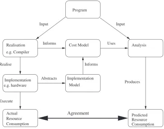
Figure 1. A general model of resource analysis.
3.1. A general model of resource analysis
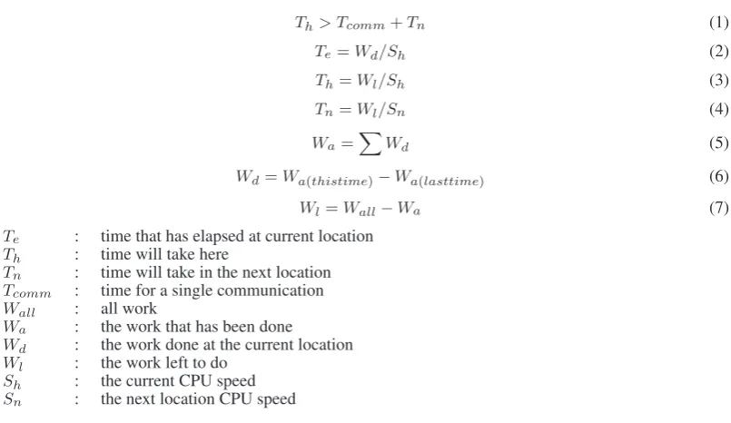
Figure 1 depicts a general model of resource prediction. The left hand side of the model depicts classical program realisation: aprogramin some language is taken as input by somerealisation, for example by a compiler or interpreter. The program is realised for some specificimplementation; for example, a compiler may generate machine code for a specific architecture, or an interpreter may execute on a specific architecture. When the program realisation is executed on that architecture, it will exhibitresource consumption. That is, it will consume a certain amount of time, memory, power and other resources, and these can (usually) be measured.
The remainder of the diagram describes the resource analysis, together with its relationship to the program realisation components. The analysis has the following components and information flows. Animplementation model specifies the resource consumption of a specific implementation. If time is the resource of interest, the implementation model might record the time to execute each instruction supported by the machine. For space, it might be the space consumed by each instruc-tion. The model may be very accurate (e.g. measuring time as a precise number of machine cycles) or very abstract (e.g. measuring time as a count of function calls).
Cost models.In model theory, a model for a formal language is aninterpretation, that is assign-ments to variables that make true some property of some set of sentences. A cost model for a programming language has a strongly related but slightly different sense of characterising some cost for an arbitrary program for arbitrary data. A good cost model thus abstracts from the full details of the executable program and operating environment, while capturing enough of their essential characteristics to enable reliable predictions of observable behaviours.
The cost model is parameterised by the implementation model to reflect resource costs on the chosen implementation. It may also be informed by aspects of the languagerealisation, for example information about the compiler optimisations used.
an analysis may use one of a variety of techniques, including type inference, abstract interpretation or abstract execution, to build a resource prediction from a cost model.
The output of the analysis is a predicted resource consumptionthat should agree, under some quality conditions, with the actual resource consumption of the program realised on the given implementation. Clearly in a worst-case analysis, it is essential that the actual consumption does not exceed the predicted consumption, but more commonly the similarity between the predicted and actual consumption is measured (e.g. the prediction is within 20% for all programs measured).
3.2. Example sequential resource analysis
We illustrate our general resource analysis model by considering a very simple sequential resource analysis. In Section 4.2, we will show how the model we have built here can be extended to cover the costs of parallel execution.
At its simplest, a model and analysis involve counting how often particular source-level constructs occur in a program execution and then multiplying these counts by some measure. For example, con-sider the toy expression languageAwith theabstract syntaxshown in Figure 2. The denotational semantics for this language is shown in Figure 3, wheresmaps variables to values, andvaluereturns integer values. Theimplementationof this language uses the simple stack machine whose pseudo-code instructions are shown in Figure 4. Programs in this language can berealisedas stack machine instructions by following the compilation rules in Figure 5. For example, we have that
compa ŒaD3.bC1/ <a7!1Ib7!2 >)
PUSHI 3I PUSHM 2I PUSHI 1I ADDI
MULTI POPM 1
We may now devise acost model that counts how often each distinct machine instruction is gen-erated, as shown in Figure 6. This cost model is informed by some model of theimplementation. In this case,INSTc is the abstract cost of machine instructionINSTon the implementation
plat-form for the resource that we are interested in. In general, the resource might be any monotonically
Figure 2. A simple arithmetic language,A.
Figure 3. Denotational semantics forA.
Figure 5. Realisation ofA: compilation rules.
Figure 6. A simple arithmetic language,A.
increasing cost such as time, dynamic memory allocation or power consumption.‡ Such abstract costs may be considered directly to explore therelativeresource consumption of program compo-nents. Alternatively, given the actual costs for each instruction on some implementation platform (e.g. derived by profiling or from the manufacturer’s specifications), we may calculate a predicted cost for a program.
ForA, the obviousanalysisis simple abstract execution of the program by using the cost model, that is anabstract interpretation[20] orsymbolic execution. We note that the analysis is of linear complexity in the number of nodes in a program’s abstract syntax tree and that it will always termi-nate because our source language has no iteration or recursion. The cost for our running example can therefore be calculated as follows:
costaŒaD3? .bC1/)
2PUSHIcCPUSHMcCADDcCMULTcCPOPMc
This section has shown how to construct a simple source-level analysis for determining the resource usage of arithmetic expressions. Our example shows how a language’s operational seman-tics and compiler realisation can guide the construction of a simpleabstract interpretationof the abstract syntax forms for our expression language. However, this analysis deals only with sequential execution costs.
4. PARALLEL/DISTRIBUTED RESOURCE ANALYSIS
This section introduces parallel/distributed resource analysis, relates it to sequential resource anal-ysis and gives an example parallel analanal-ysis. For parallel/distributed resource analanal-ysis, coordination costs are a key concern, for example the costs of communicating and synchronising between processes.
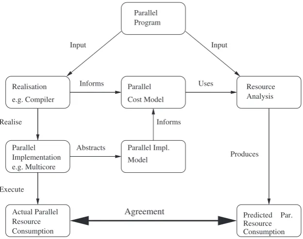
We first observe that parallel and distributed resource analyses are instances of the general resource analysis model in Figure 1. For concreteness, let us consider a parallel resource analysis as depicted in Figure 7. The information flows in the parallel model are the same as in the general model; for example, a program is realised on some implementation and consumes resources when executed.
Realisation
Realise
Execute
Uses Informs
Abstracts
Agreement
Produces Informs
Model
Predicted Resource Consumption Cost Model
Parallel
Parallel Impl.
Consumption Resource
Actual Parallel Par.
Parallel Implementation e.g. Multicore
Resource Analysis Parallel
Program
t u p n I t
u p n I
[image:8.595.141.454.67.314.2]e.g. Compiler
Figure 7. A model of parallel resource analysis.
Crucially however, the realisation, implementation, implementation model and cost model all reflect the parallel coordination aspects. For example, the realisation might compile to multithreaded code, and the implementation might support 128 cores with shared memory. The implementation model might reflect both the number of cores and the costs of creating and synchronising threads on the specific platform.§ The parallel cost model is parameterised with costs for both sequential program components and for coordination aspects such as communication and synchronisation. In general, these parameters may be obtained by abstraction, profiling, measurement or by resource analysis, as detailed in Section 7.
In contrast to the other components of the model, the analysis component of a parallel analysis typically uses standard techniques to construct the parallel resource consumption prediction. So the analysis might be constructed by abstract interpretation.
4.1. Structuring parallel resource analyses
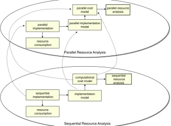
For the purposes of exposition, let us develop a parallel resource analysis informed by the sequen-tial analysis from the previous section. Although we could simply extendAand its semantics, with parallel constructs, it is generally better to separate the costs of parallel coordination from those for sequential execution. In such an approach, the parallel/distributed resource analysis is parameterised by information from a sequential resource analysis as shown in Figure 8: we have two instances of the resource analysis model in Figure 1. The parallel implementation comprises a number of sequential components, so the parallel implementation and implementation model are informed by the sequential implementation and implementation model, respectively. Similarly, the parallel cost model coordinates a number of sequential components and hence is informed by the sequential cost model.
The advantages of separating sequential and parallel/distributed analyses is that alternative sequential cost models and analyses can be used, improving the generality of the models and anal-yses, as well as allowing the reuse of sequential cost models and analyses. It also makes it possible
§denoted FORK
parallel cost model
parallel resource analysis
parallel implementation model
Parallel Resource Analysis
computational cost model
sequential resource analysis
implementation model
Sequential Resource Analysis sequential
implementation
resource consumption
parallel implementation
[image:9.595.127.473.72.327.2]resource consumption
Figure 8. A two-level model: a parallel resource analyses informed by a sequential analysis.
to reason independently about the costs of parallelism, leaving the sequential costs to be supplied through appropriate parameters in the models and analyses.
4.2. Example parallel resource analysis
We define the simple parallel language,P, that is shown in Figure 9. Parallelism is introduced by the||construct, wherep||qexecutespin parallel withq. Similarly, sequential execution is intro-duced by the;construct, wherep;qexecutes firstpand thenqsequentially. The two independent states that result from executingpand qin parallel are merged using the˚operator, whose pre-cise semantics we will leave undefined but which interleave the state changes made by pand q
(Figure 10).
Assignments in our sequential arithmetic languageAcan be directly embedded inP. We assume thatmemory is shared among all the processors but that each processor will have its own stack pointer and stack, initially empty. We therefore modify each of the stack machine operations to refer to the current processorpas shown in Figure 11. It is also necessary to introduce instructions for parallelism. Here, we use one very simple instruction,FORK, which takes two code arguments,
Figure 9. A simple parallel language,P.
Figure 11. Implementation ofP: parallel stack machine instructions.
Figure 12. Implementation ofP: fork instruction.
Figure 13. Realisation: compilation rules forP.
Figure 14. Parallel cost model I forP: execution time.
Figure 15. Parallel cost model II forP: processors needed.
task1 andtask2, and executestask1 in parallel withtask2. As shown in Figure 12, this is imple-mented using two primitives: thenew threadprimitive creates a new threadtand executes the code for that thread on an available processor; the corresponding joinprimitive waits for a threadt to terminate. The corresponding compilation rules are shown in Figure 13.
We can now build theparallelcost model shown in Figure 14, which calculates the WCET for a program inP assuming that there are sufficient processors for all tasks created. As discussed in Section 4.1, the parallel cost model builds essentially on our sequential cost model forA,costa. In our fork/join model, and with sufficient processors, the worst-case time for parallel execution is the maximum time for executing either task; the time for executing a sequential statement is just the sum of the times for the two substatements. Note that our implementation model now contains an additional coordination parameter, namely the cost of forking a new task, FORKc. The value of this
parameter might be obtained by measurement, estimation or from a detailed model as discussed in Section 7.
As for the sequential analysis ofA, the obviousanalysisforP is abstract interpretation. So for example parallel execution time can be predicted as follows.
costpŒaD3.bC1/ jj cD5)
max.2PUSHIc CPUSHMcCADDcCMULTcCPOPMc,
PUSHIcCPOPMc/CFORKc
4.3. Effectiveness of a parallel/distributed resource analysis
As we have seen, for a resource analysis to beeffective, it must have some a priori information about the language realisation. It must also have some a priori information about the target implementation platform. The latter may be obtained in a black-box way by measurement, profiling, abstract inter-pretation, and so on of primitive program constructs on the target platform. That is, constructing a good resource usage model that covers all the issues that may impact performance (whether derived from hardware, software or the operating system) is crucial to obtaining a good and useful resource analysis. Obviously, the analysis as a whole will only be effective if this basic information is good quality.
Let us return to the challenge of constructing an effectiveparallelprogram, assuming we have an effective sequential resource analysis. We can analyse the components of a program to identify which might be suitable for multiprocessor implementation and apply Amdahl’s Law to costs to check whether parallel execution might bring worthwhile benefit. However, this is only half the story. As discussed previously, if we introduce new communication and coordination constructs to enable multiprocessing, then we must also account for their costs.
The remainder of this paper is centrally concerned with different techniques for assessing paral-lel/distributed communication and coordination costs, under the assumption that adequate models and analyses are available for sequential program costs. As we shall see, such techniques depend strongly on the communication and coordination abstractions used in both programming languages and runtime systems and vary substantially in the degree of detail that they consider and in the precision that they offer.
5. CONSTRAINED PARALLEL/DISTRIBUTED PROGRAMMING PARADIGMS
Many parallel/distributed programming paradigms are constrained, typically to simplify program-ming. This section briefly outlines why and how parallel/distributed programming paradigms are constrained and surveys some important constrained paradigms that are covered in subsequent sections.
As we have seen in Section 2, parallel/distributed programming can be difficult because in addi-tion to solving the challenges of specifying a correct and efficient algorithm, the programmer must also specify the effective coordination of the program components. A number of programming paradigms exist that attempt to ease the challenges of parallel/distributed software engineering by constraining the coordination model but, crucially,notthe computation model, so the paradigms remainTuring complete.
Many of these constrained parallel/distributed programming models simultaneously make the resource analysis of programs more tractable. For example, the programming models may constrain the programmer to usespecific coordination patterns, such as algorithmic skeletons, or the program-mer to use a singlecoordinationpattern, such as the bulk synchronous parallel (BSP) model. In both cases, this guides the choice of specific cost models, as we will see in the following section.
5.1. Bulk synchronous parallel
The BSP model constrains the programmer to a single coordination pattern that formulates compu-tations as a series ofsupersteps[21]. A BSP computer comprises a number of parallel processors connected by a communication network. Each processor has a local memory and may follow its own thread of computation. Each superstep in the BSP computation comprises three stages:
Independent concurrent computationon each processor using only local values.
Communicationin which each processor exchanges data with every other processor.
Barrier synchronisationwhere all processes wait until all other processes have finished their communication actions.
5.2. The Bird–Meertens Formalism
The Bird–Meertens Formalism (BMF) [22] constrains the programmer to use a fixed set of higher-order functions (HOFs). BMF is a calculus for deriving functional programs from specifications, with an emphasis on the use of bulk operations across collective data structures such as arrays, lists and trees. Although independent of any explicit reference to parallelism, many of its opera-tions clearly admit potentially efficient parallel implementation. We discuss BMF cost models in Section 6.6.
5.3. Parallel and distributed skeletons
Skeletons constrain the programmer to use a fixed set of commonly occurring coordination pat-terns [23]. The patpat-terns are abstracted as library or language constructs that implement the coordi-nation. More precisely the skeletons are HOFs¶ that the application programmer instantiates with
sequentialcode. For example, a parallelmapfunction will apply any sequential function to every element of a collection in parallel. The programmer’s task is greatly simplified as they do not need to specify the coordination behaviour required.
The skeleton model has been very influential, appearing in parallel standards such MPI and OpenMP [24, 25], and distributed skeletons such as Google’s MapReduce [26] are core elements of cloud computing. We discuss cost models for skeleton-based approaches in Section 6.7.
5.4. Workflow languages
Workflow description languages such as Business Process Execution Language [27] or Pegasus (planning for execution in grids) [28] constrain the programmer to use a small set of process struc-turing constructs such as sequencing and parallelism. Whereas the computations coordinated in the workflow are almost invariably expressed in a Turing complete language, the process structuring constructs provided by most workflow languages are not Turing complete; for example, they may lack iteration.
6. PARALLEL AND DISTRIBUTED COST MODELS
Cost models for parallel and distributed execution range from theoretical models that are aimed at studying algorithmic complexity, such as the parallel random access machine (PRAM) model, down to highly concrete models that may help with static task mapping or dynamic scheduling decisions. In this section, we survey a number of well-known and representative cost models that are used in the analysis methodologies that we will present in Section 8. A more detailed survey of parallel cost models is given in [29].
As shown in Figure 1, cost models for parallel or distributed execution are generally structured as two-level models: theimplementation modeldetermines execution costs for individual operations; thehigh-level modelthen synthesises the overall system costs from the implementation level costs, given some parallel execution model for the system as a whole. As we shall see in Section 9, classi-cal sequential cost models can also be useful here, for example in using the predicted execution time for tasks to inform scheduling decisions. Clearly, where a high-level model is built on a low-level one in this way, any inaccuracies in the low-level model will be reflected in, and perhaps magnified by, the high-level model. It is therefore vitally important that the low-level cost model is sufficiently accurate to allow good costs to determined by the high-level model and that the high-level model takes into account any vagaries or deficiencies of the low-level model that could be magnified in the final combined analysis.
6.1. The parallel random access machine model
The PRAM model [30] is a highly abstract model of parallel computation. It is widely used within the parallel algorithms and complexity research community as a standard theoretical model of a parallel machine, occupying a status similar to that of the Turing machine. By abstracting over primitive PRAM operations, it is possible to derive a standard measure of the parallel complexity of a program. The resulting model is a very general one. In fact, it has even been suggested that PRAM should form a general model of computation, both sequential and parallel [31].
In its simplest form, the PRAM model enforces stepwise synchronous, but otherwise unrestricted, access to a shared memory by a set of conventional sequential processors. At each synchronous step, every processor performs one operation from a simple, conventional instruction set. Each such step is costed at unit time, whatever the operation, and regardless of which shared-memory locations are accessed.
For example, given the problem of summing an array ofnintegers on ap-processor machine, a simple algorithm A might first sum a distinct subarray of sizen=pitems on each of thep proces-sors and then use a single processor to sum all theppartial results from the first phase. An informal PRAM cost analysis would capture the cost of this algorithm as follows:
TA.n/D‚
n pCp
A more sophisticated algorithm B might instead sum the partial results in a parallel tree-like struc-ture (usually known as ‘parallel reduction’). An informal PRAM analysis would capstruc-ture this cost as follows:
TB.n/D‚
n
pClogp
These analyses clearly show that although algorithm B is asymptotically faster than algorithm A, as intended, this is only true for largep.
Although the basic PRAM model provides a durable and sound basis for at least the initial phases of parallel algorithm design, it ignores a number of important issues such as contention, the memory hierarchy, the underlying communication infrastructure and all internal processor issues. Several variants of the basic PRAM model that aim to address these and other pragmatic cost issues have been introduced. For example, the exclusive-read-exclusive-write PRAM model disallows steps in which any shared-memory location is accessed by more than one processor (algorithms A and B both satisfy this requirement). In contrast, the concurrent-read-concurrent-write PRAM model removes this restriction, with subvariants defining the required behaviour when clashes occur.
6.2. Parallel random access machine models for multicore machines
The PRAM model described previously has been one of the most influential parallel cost models. Because it is highly idealised, for example assuming zero-cost memory access, it is a good basis for adesign-timeanalysis (i.e. a manual complexity analysis that is performed by the parallel algorithm designer), where it can be used to expose the maximum parallelism in the algorithm. However, it does not reflect many of the important costs incurred when executing the algorithm on a real parallel machine. Several refinements of this highly abstract model have been suggested, for exam-ple the hierarchical PRAM [32], local memory PRAM [33] and block PRAM [34] models.||These variants add the concepts of data locality and remote memory, with varying memory access costs, to the basic PRAM model. Even more detailed are the Parallel Memory Hierarchy (PMH) [35] and Parallel Hierarchical Memory [36] models, which model the entire memory hierarchy. For PMH, the memory hierarchy is modelled as a tree, whose nodes represent memory and whose leaves rep-resent processors. The cost of data transfer in this model is reprep-resented as the length of the path
between two nodes in the tree. Parameters that characterise the (memory) nodes are the block size, the number of blocks and the transfer time (latency) to neighbouring nodes. This design permits modern, deep memory hierarchies to be accurately modelled.
6.3. Cost models for hierarchical parallel machines
All of these models assume the use of a shared memory, albeit with varying memory access costs. A different class of models has been developed for dealing with distributed memory systems, as found in clusters or clouds. In these models, a conceptual distinction is made between accessing memory locally and transmitting data over a network. The key system characteristics that are commonly modelled in such models include the following:
Degree of parallelism: the number of processors available.
Latency: the time between sending a message on one processor and receiving it on another processor. In modern architectures, this usually depends on the depth of the hierarchy.
Memory access: the cost of reading or writing to a memory location. In modern architec-tures, this usually depends on the location in the hierarchy.
Synchronisation: the costs of synchronising a group of processors.
Bandwidth: the amount of data that can be sent within a given time interval.
One of the best known models is LogP [37], which models the costs of data transfer across a network using the following parameters:
L (‘latency’) – the variable amount of time that is needed for communication between two processors.
o(‘overhead’) – the fixed amount of time that is needed to prepare for sending or receiving messages.
g (‘gap’) – the minimal interval between sending two messages (this is the inverse of the bandwidth).
P (‘processors’) – the number of processors on the machine.
The LogP model has proven to be a good compromise between very abstract, simplifying models such as PRAM, and very concrete and detailed models of homogeneous networked architectures. Like the PRAM model, it is mainly used as basis for a design-time analysis. One limitation to the LogP model is that it assumes a homogeneous architecture, where the costs of communication are the same between all processors in a system. Although this may be true for a single cluster, it will generally not be the case for computational grids or cloud computers. An extension of the LogP model, HLogGP [38], has been developed that uses vectors of the LogP parameters to model heterogeneous architectures, such as these. This model has been shown to deliver good predictions on heterogeneous clusters.
We now use the basic LogP model to analyse the costs of our example program of computing the sum over an array of lengthnonP processors, using list-structured communication. In the LogP model, we have to account for the overhead involved in sending a message and the gap between sending messages. We assume0costs for splitting the array into chunks of sizedn=Peandasteps as cost for performing an addition. In the broadcast phase of the algorithm, assumingo < g, the root processor sends chunks of the array at stepo,oCg,oC2g,: : :in the execution. The last chunk is sent at step oCg .dn=Pe 1/. AllP processors do their summations in parallel. The cost of the summation over one chunk isc Da .dn=Pe 1/. Computation can begin at stepoCLafter sending it becauseLsteps are needed for the transmission andosteps for receiving the data. The result of the computation is sent at stepoafter finishing the computation. Thus, the processors send their results at steps3oCLCc,3oCLCgCc,: : :back to the root processor. The last message arrives at4oC2LCcCg .dn=Pe 1/steps because it takesLsteps to arrive andosteps to process. Computing the overall sum overP partial sums takesaP steps. Thus, the total time for computing the result, based on list-structured communication, is4oC2LCcCg .dn=Pe 1/CaP.
parameters for the communication overhead and the gap between sending messages, representing a limit on the bandwidth, give a more realistic picture of the execution and avoid an algorithm design that makes excessive use of interprocessor communication.
6.4. System-oriented cost models
The implementation models that are described in Section 7 can be used to provide detailed infor-mation about the costs of coordination operations on a given hardware. Such models are often used in hardware design to capture the characteristics of a parallel machine and to compare idealised performance profiles. They are less attractive as a computational model, however, because they expose many machine-level details to the program and may therefore make it considerably more complicated.
The role ofsystem-orientedcost models is to capture the costs imposed by software-level sys-tem operations, for example the costs of thread creation. In typicalbridging models, all such costs are subsumed into a small set of parameters. This simplifies the manual, design-time analysis of algorithms. In contrast, capturing system costs in a separate system-oriented cost model provides additional information that can be used during runtime to control the management of the parallelism. In particular, for systems that perform automatic load balancing, where tasks are dynamically moved between processors to equalise the load on each processor, this provides important input to the decision about where a thread should be executed.
In terms of precision, then, system-oriented cost models form an intermediate step between archi-tectural cost models and computational cost models. They are mainly used to construct runtime analyses that can advise a suitably adapted runtime system. For example, they may be used to guide one of the following dynamic resource policies:
Load distribution: this aims to spread the available parallelism evenly among all processors, with the objective of achieving optimal utilisation of the parallel machine.
Data locality: this policy aims to keep logically related threads on the same processor to reduce communication costs.
Scheduling: this policy decides which of the runnable threads to execute next on a given processor.
The following example illustrates how a simple system-oriented cost model can be used to auto-matically control the load-balancing policy for a heterogeneous architecture. A good strategy for load balancing for tightly coupled multicore processors is to send work to a processor with the high-est relative speedRiDSi=Wi, whereSiis the speed of processoriandWiis its current load. Thus,
work should be transferred from processorj to processoriso that
8m.m2 f1 : : : ng,j 6Dm)
.Rm6Ri/ ^
kRj 6Ri
A throttling factorkis used to avoid overly aggressive work redistribution.
6.5. The bulk synchronous parallel cost model
The BSP model outlined in Section 5.1 occupies a more concrete position in the cost model spectrum than the PRAM models described previously. Like the basic PRAM model, BSP uses a synchronous stepwise model of parallel execution. In contrast to the basic PRAM model, however, the BSP model recognises that synchronisation is not free, that sharing of data involves communication (whether explicitly or implicitly) and that the cost of this communication, both in absolute terms and rela-tive to that of processor-local computation, can be highly machine dependent. It also generalises the sequential computations to be any required computation rather than a small set of primitive operations.
The BSP cost model has two parts: one to estimate the cost of a superstep and another to estimate the cost of the program as the sum of the costs of the supersteps. The cost of a superstep is the cost of the longest running local computation, plus the largest cost of communication between the pro-cesses, plus the cost of the barrier synchronisation. The costs are computed in terms of three abstract parameters that respectively model the number of processorsp, the cost of machine-wide synchro-nisationLandg, a measure of the communication network’s ability to deliver sets of point-to-point messages, with the latter two normalised to the speed of simple local computations.
For example, the array summing algorithms, translated for BSP, would have asymptotic run-times of
TA.n/D‚
n
pCpCpgC2L
where the first two terms are contributed by computation, the third term is contributed by communication and the fourth term is contributed by the need for two supersteps, and
TB.n/D‚
n
pClogpC2glogpCLlogp
where the first term corresponds to local computation, and the other three terms to computation, communication and synchronisation summed across the logp supersteps of the tree-reduction phase. This analysis clearly reveals the vulnerability of the algorithm B to architectures with expensive synchronisation costs, that is a largeL.
This constrained model of parallel computation allows BSP implementations to provide a bench-mark suite that derives the implementation model, that is the machine-specific values for the four BSP parameters. These can then be inserted into the abstract (architecture independent) cost derived already for a given program to predict its true performance.
Whereas the BSP model makes no attempt to account for processor internals, the memory hier-archy (other than indirectly through benchmarking) or, for specific communication patterns,** a considerable literature testifies to the pragmatic success of the approach [39]. A primary limitation is that because the cost of a superstep is governed by the worst-case cost of any local computation, the BSP model is only suitable for computations where each superstep is fairly regular, that is where thegranularityof each local computation in a superstep is broadly the same.
6.6. The Bird–Meertens Formalism cost model
A number of authors have investigated adding parallel cost analyses to the BMF-inspired program-ming models that were outlined in Section 5.2. Two examples are described in the following.
BMF-PRAM: In [40], Cai and Skillicorn present an informal PRAM-based cost model for BMF
across list-structured data. Each operation is provided with a cost, parameterised by the costs of the applied operations (e.g. the element-wise cost of an operation to be mapped across all elements of a list) and data structure sizes, and rules are provided for composing costs across sequential and concurrent compositions. The paper concludes with a sample program derivation for themaximum segment sumproblem. In conventional BMF program-calculation style, an initially ‘obviously’ cor-rect but inefficient specification is transformed by the programmer into a much more efficient final form. For our array summing problem from Section 6.1, algorithm A would be expressed as amap
across the partitioned input list, followed by a sequential second phase (perhaps concealed as a further degeneratemapacross a list with only one member, itself the list of partial sums). Analy-sis would return the result described in Section 6.1, being the sum of the costs of the two phases. The cost of the first phase would emerge from analysis of the mapped function (summing a sub-list) and the generic cost of a parallelmap, being the product of the cost of one instantiation of the mapped function (heren=p) and the number of such calls assigned to each processor (here one).
Similarly, for algorithm B, the second phase would be expressed as a parallelreduceand thereby analysed to cost log ptimes the cost of the reduction operator (here addition, therefore costing unit PRAM time).
Similarly, in [41], Jayet al.build a formal cost calculus for a small BMF-like language using the PRAM model as the underlying cost model. For implementation to be aided, the language is further constrained to beshapely, meaning that the size of intermediate bulk data structures can be statically inferred from the size of inputs. The approach is demonstrated by automated application to simple matrix–vector operations. These approaches can be characterised as being of relatively low accuracy (a property inherited from their PRAM foundation), offering a quite rich, although structurally constrained source language, being entirely static in nature and with varying degrees of formality and support.
BMF-BSP: Building on the seminal work described previously, a number of authors have sought
to inject more realism into the costing of BMF-inspired parallel programming frameworks by sub-stituting the BSP model for the PRAM model [41, 42]. In particular, [42] defines and implements a BMF-BSP calculus and compares the accuracy of its predictions with the runtime of equivalent (but hand-translated) BSP programs. With the utilisation of maximum segment as a case study, the predictions exhibit good accuracy and would lead to the correct decision at each stage of the pro-gram derivation. For our array summing problem, the analysis would return a concrete prediction, composed similarly to the discussion in 6.5 but embedding concrete BSP cost values for the chosen architecture. Meanwhile, in a more informal setting reflecting the approach of [40], Bischofet al.
[43] report on a BSP-based, extended BMF derivation of a program for the solution of tridiagonal systems of linear equations. Once again, good correlation between (hand-generated) predictions and real implementation is reported, with no more than 12% error across a range of problem sizes. These developments can be characterised as offering enhanced accuracy, while retaining similarly structured models and support. As a by-product of the use of BSP, analyses can now be made spe-cific to the target architecture once they are instantiated with the standard BSP constants for that architecture.
6.7. Skeletons
Theskeleton-based approach to parallel programming outlined in Section 5.3 advocates that com-monly occurring patterns of parallel/distributed computation and interaction should be abstracted as library or language constructs. Several authors have sought to associate cost models to algorithmic skeletons and to use these either explicitly or implicitly to guide the development and implemen-tation of parallel programs. Few authors, if any, have considered the more complex issue of cost models for distributed skeletons.
For example, on the basis of a simple model of message passing costs, Hammondet al.[44] use metaprogramming to build cost equations for a variety of skeleton implementations into a skele-ton library for the parallel functional language Eden. This approach allows the most appropriate parallel implementation to be chosen at compile-time given instantiation of some target machine-specific parameters. The paper shows how these parameters can be used to discriminate between four possible parallel variants of a farm skeleton for a Mandelbrot visualisation problem.
Meanwhile, Gava [45] describes an attempt to embed the BSP model directly into the functional programming language ML. At the level of parallelism, the programming model is thus constrained to follow the structure of a BSP superstep (a relatively loose skeleton), whereas computation within a superstep is otherwise unconstrained. Analysis is informal, in the conventional BSP style, but the language itself has a robust parallel and distributed implementation. A reported implementation of ann-body solver once again demonstrates close correlation between predicted and actual execution times.
strategies are evaluated, and the best is then selected. In a novel extension, designed to cater for sys-tems in which architectural performance characteristics may vary dynamically, the chosen model is periodically validated against the actual runtime performance. Where a significant discrepancy is found, the computation can be halted, re-evaluated and rescheduled.
Consider again the problem of summing an array ofnintegers onpprocessors. The idealised data-parallel skeleton is as follows:
void FARM(int p, int work(int *,int), int *input,int n,int *output)
wherepis the number of processors,workis a worker function taking an integer array argument to an integer result,input is the input array of integers, n is the size of theinput array and
output is the output array of lengthp.FARMsends a chunk of sizen/pfrominput to each of thepprocessors, which applyworkto the chunk. Processorjreturns aninttoFARM, which stores it inoutputsat positionj. Given
int sum(int *a,int n) { int i,s;
s=0;
for(i=0;i<n;i++) s=s+a[i]; return s; }
we might call
int A[N],O[N]; ...
FARM(P,sum,A,N,O); result = sum(O,P);
to sum arrayAof lengthNonPprocessors via arrayO. Suppose that for some distributed memory parallel architectures, where every node has the same characteristics,
sendint.n/ is the cost of sending/receivingnints from/to farmer to/from worker;
processsum.n/ is the cost of applyingsumton ints.
Then the predicted execution timeTA.n/will be
p sendint.n/p/C
processsum.n/p/C
p sendint(1)C
processsum(p)
The coordination terms of such cost expressions must be simplified with care. For example, in the equation above, message latency almost certainly means that the cost of sending two messages –
se ndint .n=p/Csendint .1/ – is very different from sending one, slightly larger message –
sendint.n=pC1/.
7. IMPLEMENTATION MODEL
Some implementation parameters of parallel/distributed cost models are readily available as static characteristics of the target architecture. For example, many parallel cost models are parameterised by the number of processors available. Other parameters are harder to determine, for example the communication latency fornunits of data.
Some implementation parameters can be determined using techniques that are well established in the sequential resource analysis community, for example execution time, or memory consumption predictions. For completeness, we briefly discuss these techniques in the following.
Other implementation parameters are specific to parallel/distributed cost models, for example communication costs or synchronisation costs, denoted asLand gin the BSP model. The tech-niques for determining the values of these specialised implementation parameters are, however, broadly similar to determining the parameters for sequential cost models, namely estimation, pro-filing/measurement or detailed models. This section outlines these approaches and gives references to examples of the techniques in practice in Section 9.
7.1. Estimation
One very simple approach, suitable for abstract cost models, is to abstract over most of the details involved in the parallel execution and to only provideestimatedvalues for the parameters. Although not providing realistic costs, such a model can be useful in providing relative information, for exam-ple on the degree of communication involved in an execution. This simplified realisation is used in early execution time analyses such as [48, 49].
7.2. Measurement-based approaches
A more scientific approach, and one that more accurately determines the cost model parameters, is to measure the parameter of interest on the target implementation. Commonly, a suite of representative example applications are eitherprofiledorinstrumentedto measure the parameter value. For exam-ple, Section 9.1 shows how profiling is used to predict parallel execution times, and Section 9.2.3 contains examples showing how instrumented programs are used to determine the computation and communication parameters for a distributed cost model.
For cost model parameters to be determined more easily and more reliably, some libraries pro-vide ready made instrumentation benchmarks to be run on a new architecture, for example [21, 46]. However, both profiling and instrumented programs can suffer from the problems of accuracy and generality that are described in Section 2.
One way of overcoming the accuracy and generality issues is described by Bonenfantet al.[50], who have measured costs of bytecode instructions for an abstract-machine implementation. Because well-constructed bytecodes will expose all the interesting cost parameters, and all possible execu-tion paths can be measured for each individual bytecode, this approach allows a relatively small number of measurements to cover the costs of all possible program executions by combining the costs of the individual bytecodes to reflect the execution paths for a particular program. Although issues of cache and pipeline behaviour, and so on can have an impact on the accuracy of the analysis for more complex processor architectures, the approach is promising for abstract-machine imple-mentations, giving a cheap yet general and fairly accurate methodology for determining program execution costs.
7.3. Detailed models
An even more accurate prediction of a parameter value can be obtained by using a detailed model. Detailed models may be constructed for a range of resources, for example memory or time.
For accuracy, such models need to account for the complete state of the processor, including, for example, its caches and pipelines.
Whereas many uses of resource analysis do not need such a precise model, this level of detail and accuracy is required for industrial-strength WCET analyses. A detailed survey of WCET anal-yses is given in [51]. Because these analanal-yses are used to guarantee the safety of real-time systems, such as flight controllers or automotive safety systems, WCET analyses must besafein the sense of always producing upper bounds on execution time. A secondary concern is that WCET analyses should be as precise as possible to avoid over-specifying processor requirements, with consequent cost implications. One example of a WCET analysis that combines these features is AbsInt’saiT
tool that produces worst-case timing information for sequential C code fragments for a number of processor architectures [52]. The use ofaiTas part of an analysis giving execution time bounds is outlined in Section 9.3.2.
7.4. Determining memory usage and other costs
The aforementioned discussion has focused on execution time. Generally, this is the resource that is of most interest in parallel or distributed programming. It is also one of the most diffi-cult resources to obtain accurate information about because time usage may be nondiscrete and nonmonotonic, depending on detailed contextual information, including the dynamic state of the processor, such as the caches or pipeline states. In the worst case, it may even be nondetermin-istic! For example, two cores may impact each others execution times by executing threads that share the same cache. The effect depends on the precise timing of the two threads and the precise hardware implementation. In contrast, memory usage tends to be deterministic and may often be monotonic.
Most of the models and techniques described previously can also be used to determine memory or other resource usage costs with small modifications. For example, Hofmann and Jost originally applied an amortised cost analysis to determine linear bounds on heap allocations and deallocation for a first-order functional language, including recursion [10], and this work has subsequently been extended to cover stack usage [53, 54] and WCET costs [12, 54]. This work has been exploited in the EmBounded project funded by the European Union to produce formal cost models and analyses for heap, stack and time usage for the Hume language (http://www.embounded.org). The amor-tised cost approach that is used in this work aims to even out costs across different operations. This cost can then be used to assign weights in the types of functions, and so on that reflect the costs of different cases in the input and result data structures.†† Thus, the cost of a function or program can be determined in terms of the sizes of its input and result data structures. A com-plementary type-based approach can be used to infer thesizesof data structures. Chin and Khoo [55] introduced a type inference algorithm that is capable of computing size information from high-level program source. Vasconcelos and Hammond use a similar technique to infersized typesfor recursive, polymorphic and higher-order programs [56]. Vasconcelos’ PhD thesis [9] extends these approaches using abstract interpretation techniques to automatically infer linear approximations of the sizes of recursive data types and the stack and heap costs of recursive functions. By including user-defined sizes, it is possible to infer sizes for algorithms on nonlinear data structures, such as binary trees.
A number of authors have also recently studied analyses for heap usage in an imperative setting. Albertet al.[57] present a fully automatic, live heap-space analysis for an object-oriented bytecode language with a scoped-memory manager. This analysis is not restricted to a certain complexity class but unlike the amortised cost approaches, for example, cannot express data dependencies. Brabermanet al.[58] infer polynomial bounds on the live heap usage for a Java-like language with automatic memory management but do not cover general recursive methods. Finally, Chinet al.[59] present a heap and stack analyses for a low-level (assembler) language with explicit (de)allocation, which is also restricted to linear bounds.
8. CONSTRUCTING RESOURCE ANALYSES
A resource analysis uses some cost model to synthesise a prediction for the execution costs of the given program on some implementation platform, as depicted in Figure 1. This section discusses the techniques used to construct resource analyses in each of the three phases of a program’s lifetime: design, compilation and execution (runtime).
This section provides only an overview of analysis methods, as they are generic and well estab-lished. That is, rather than being specific to resource analysis, methods such as abstract interpretation or constraint system solving are used in many domains for many different purposes. In consequence, they are covered relatively briefly here, with citations to important papers detailing the analysis methods.
8.1. Design-time analysis
Abstract cost models such as those based on the PRAM [30] model, and to some extent those based on the BMF or BSP models, enable the programmer to reason about costs during program design. Such models often require that the program is expressed using a specific structure, for example as a sequence of supersteps for BSP analysis, or using only the BMF operators to express parallelism. Here, the resource analysis is typically not automated, and the relatively simple cost models enable the programmer to perform the resource analysis using pen and paper. A significant advantage of design-time analysis is that guided by the predictions produced by the analysis, the programmer can relatively cheaply transform the program design before committing to a specific implementation.
A commonly used asynchronous, distributed cost model is LogP [37]. It models the costs for data transfer using the following parameters:L, the latency in sending a message between two machines;
o, the overhead of composing and sending the message;g, the minimal gap between sending two messages (this corresponds to the inverse of the bandwidth); andP, the number of processors of the machine. This model has proven to be a good compromise between an abstract, user-friendly model of representing a homogeneous, flat parallel hardware and a more accurate machine model that accounts for interprocessor communication costs.
Being used at design time and nonautomated, these models are deliberately simple. However, for precision to be improved and in particular for more complex parallel hardware to be modelled, several extensions to these basic models have been developed. Extensions that include a hierarchi-cal memory structure to the basic machine model include the following: hierarchihierarchi-cal PRAM [32], local memory PRAM [33], PMH [35], LogP [37], HLogGP [38] and LogP-PMH [60]. All of these models aim to provide more realistic costs of memory access in a hierarchical memory model and typically view communication as a generalisation of memory access.
Design-time models are also used to improve the coordination of distributed applications. For example, high-level Petri Nets have been used to describe the workflow and resource consumption of complex Grid applications [61].
8.2. Compile-time (static) analyses
Several techniques have been developed that are capable of statically inferring information about runtime resource requirements. The best known of these are a range of compile time analyses exist, primarily type inference, abstract interpretation and constraint system solving. These tech-niques may be used either individually or in some combination. Nielsonet al.[62] provide detailed coverage of these techniques.
Type-and-effect systems. Type-and-effect systems are based on the observation that type inference can be separated into two phases: (i) collecting constraints on type/resource variables and (ii) solving these constraints [63]. Several type-and-effect analyses have been developed that extend standard Hindley–Milner type inference to collect constraints on resources, for example [64–67].
check the unannotated types and while doing so collect constraints on the annotations. For infer-ring resource bounds, these constraints are typically (in)equalities over integer or rational numbers. An additional phase then solves the collected constraints to produce resource bounds. This strand of work has been extended to higher-order sized types [70] and combined with a type-and-effect system, performing region analysis, to give resource bounds on dynamic memory consumption [71]. A concrete example of a type-based analysis is the resource analysis for the Hume language presented in Section 9.3 and discussed in detail in [12]. In this case, however, the meaning of the annotations, which are attached to type constructors, is different from those in sized types. They encode an (linear) upper bound on the resource consumption, of an expression, but not a bound on the size of a data structure. The main advantage of this different meaning of the annotations is improved compositionality of the analysis. Furthermore, it avoids the usage of a max-plus-algebra as underlying representation for resource bounds (with the max operator representing the cost of a conditional) and allows the usage of a fairly simple linear program (LP) solver to find a solution for the collected constraints. Finally, attaching all necessary resource information to a type achieves good modularity because the resource analysis only has to examine the type, not the source code, to extract the relevant information from a function possibly defined in a different module.
Abstract interpretation. Abstract interpretation [20] defines an abstract domain of values, which is typically very small and which is often used to provide purely qualitative information. For example, in strictness analysis, the interesting distinction is simply whether or not an expression is strict and therefore safe to be evaluated before passing its result to a function. By using a richer abstract domain, quantitative information, such as resource consumption, can also be modelled. Functions are mapped to abstract versions of those functions that operate over the abstract domain. The anal-ysis then proceeds by executing these abstract functions and in particular finding fixpoints for recursive functions.
One common problem of abstract-interpretation-based analyses is the need of a finite, and in prac-tice small, abstract domain to guarantee fast termination of the fixpoint generation. This often leads to an extremely simple model of resources, which in turn delivers relatively inaccurate information. This problem of domain size is even more pronounced in the presence of HOFs, which give rise to an exponential increase in domain size. One of the main advantages of abstract interpretation is the fact that many practically useful optimisation techniques have been developed for this process. Con-sequently, well-developed inference engines that can be used for cost analysis exist, for example the COSTA system [72] and the SPEED system [73]. COSTA is generic with respect to the resources that can be analysed, produces high-quality bounds that are not restricted to a particular complexity class and builds on a high-performance inference engine. A combination of this static approach with a runtime, profiling approach is presented in [74]. AbsInt’saiTtool [52], which was described pre-viously, uses abstract interpretation over machine-code fragments derived from C program source, synthesising hardware-level information to give guaranteed bounds on WCET. For accurate bounds to be obtained, the analysis uses a detailed implementation model including the cache behaviour and pipeline structure of the processor.
Section 4.2 gives two very simple examples of parallel resource analyses constructed by abstract interpretation, as shown in Figures 14 and 15. In the first, the abstract domain is execution time, and in the second, the abstract domain is number of processors. A more realistic example is the autonomous mobile program (AMP) analysis outlined in Section 9.2.2 and discussed in detail in [75]. This analysis uses abstract interpretation on a cost semantics for a subset of the Jocaml mobile programming language.
Constraint system solving. Constraint-solving approaches are related to the type inference
approaches in that they separate the collection of (general) constraints and the solution of these constraints into different phases. However, this process is not necessarily tied to type inference itself. An example of this approach are several variants of control flow analyses [76, 77].