From physical models to well founded control

From physical models to well-founded control

Simon Dobson∗

∗_{Lero, the Irish Software Engineering Research Centre}

and

Clarity, the Centre for Sensor Web Technologies UCD Dublin IE

Email: [email protected]

Lorcan Coyle †, G.M.P. O’Hare†

† _{Clarity, the Centre for Sensor Web Technologies}

UCD Dublin IE

Mike Hinchey‡

‡_{Lero, the Irish Software Engineering Research Centre}

University of Limerick IE Email: [email protected]

Abstract

Mobile sensors are an attractive proposition for environ-mental sensing, but pose significant engineering problems. Not least amongst these is the need to match the behaviour of the sensor platform to the physical environment in which it operates. We present initial work on using models of physical processes to generate models for autonomic control, and speculate that these can be used to improve the confidence we can place in sensed data.

1. Introduction

Wireless sensor networks (WSN) provide a fertile ground for autonomic systems research, since they must almost by definition operate for long periods with little or no direct hu-man supervision. This raises several important engineering questions: How can we express the tactics and strategies the nodes should use to respond to changes? How can we be assured that these approaches are, and will remain, valid? And – most importantly – how can we be sure that the sensor data we receive is valid and representative, and has not been adversely affected by the management approach we have used?

Of particular concern is the sub-field of WSNs involving mobile sensors, used when the environment is inherently mobile (such as for space probes, river and estuarine sensing) or there is insufficient coverage from a network of static sensors (as if often the case in oceanic environments). From an engineering perspective, we need to ensure that mobility improves the data stream whilst also meeting other constraints.

In this paper we present some initial investigations we are conducting into using physical models to generate autonomic control for mobile sensor networks. The basic intention is to allow us to express the tactics we use for moving sensors in terms of the physical phenomena we are endeavouring to sense. As well as making control actions easier to formulate, we believe that such a close integration between sensor and phenomenon will increase the confidence we can have in the resulting sensor data received.

Section 2 spells-out the challenge in more detail. Based on this, section 3 discusses how a physical model could potentially be used to induce a control model, and explores how multiple tactics might be expressed and validated within such a derivation. Section 4 concludes with our plans for the future.

2. The challenge

A sensor network performs two closely-entangled func-tions. Firstly, it collects data from its environment using a range of sensors, and makes this data available in some way to its managers or to the wider internet. Secondly, it manages its own operation so as to maintain its function, typically including its network connections and power management. The entangling comes from the interplay between these two goals. The data being sensed may affect management, for example by causing more readings to be taken, and more power expended, during “interesting” events. Conversely, reduced connectivity may reduce the need for, or point of, making some sensor readings such as those involving video data that cannot then be transmitted. Defining control software for such systems therefore involves substantial multi-objective optimisation.

Collect

Decide

Act _Analyse

Environmental sensorsNetwork instrumentation Application requirements User context

Uncertain reasoning Inference

Bounds and envelopes

Decision theory

Game theory Economic models Rules and policies

Hypothesis generation Inform users

or administrators Record strategies Managed elements

Risk analysis

Figure 1. The autonomic control loop (from [5])

Entangled goals are even more in evidence in situations where the sensors are deliberately mobile, and where their movement may be governed (or at least influenced) by the data being sensed. Such situations include space exploration, where the space probes may seek to avoid dangerous situa-tions, and aquatic environments in which one cannot achieve adequate coverage of an area from a fixed network of sensors for fear of interfering with other, simultaneous uses of the area. In both cases we need to have a clear link between the environment being sensedand themotion or management of the sensor in that environment.

Autonomic systems [5], [7] provide a clear conceptual model within which to address such issues. An autonomic system integrates the observation of an environment with decision-making, and “closes the loop” of control to allow later decisions to observe the impact of earlier ones (fig-ure 1). In our applications, sensing includes both data on the system’s own operation and environment, and on the phenomena it is intended to sense for its users.

2.1. Sensor swarms

Substantial experience – at least at the concept stages – exists in the autonomic control of space missions [11] and underwater exploration [6].

Our particular area of current interest is in aquatic en-vironments, including river, estuarine and marine scenarios. Sensing such environments is vitally important in order to monitor and manage pollution incidents, fish stocks, climate change, leisure use and so forth. Without reliable, long-term data collection it is impossible for scientists and policy-makers to make accurate predictions about the evolution of the environment, and to assess the impact of proposed changes upon this evolutionary process.

Such areas typically support multiple simultaneous uses, for example recreational sailing, commercial fishing and

industrial water recycling, Many of these activities have substantial economic significance – sufficient to preclude any interference with them by sensors. The sensor network must therefore be inconspicuous in order to allow use of the area, but of sufficient temporal and spatial resolution to support the tasks being demanded of it.

One approach to achieving this balance to deploymobile sensors, either passive (move with the current) or active (move under deliberate control, although perhaps under quite tight constraints). The sensor network may be sparse, and therefore unlikely to interfere with other activities; alter-natively it may actively avoid interfering by (for example) attempting to stay in “quiet” parts of the area.

Techniques for constructing and managing networks in such environments exist (see for example [10]), as well as for using mobile sensor nodes to achieve coverage of an area [3]. However, these are insufficient for the construction of a multi-sensor, “swarm” solution.

2.2. Deliberate entanglement

If we adopt the architecture of a swarm of mobile sensors that move deliberately to avoid interference, we must address some complex interactions between the mission goals, the sensed environment and the management of the sensor network.

The mission goals provide the requirements for the mis-sion, and also provide a rubric within which to evaluate its success or compare potential tactics we might deploy to manage the WSN. If, for example, the mission goal is to detect illegal pollutants in a particular estuary, this provides a requirement to search for particular sensed conditions (and potentially ignore others); we can also compare the results of the WSN against a ground truth of what incidents were detected by other means. Of course this ground “truth” will typically only be a partial view of reality, which makes impartial evaluation a hard problem.

Typically there will be trade-offs to be captured in some way. Balancing long mission life against high-resolution sensing, for example, almost certainly involves compromise; similarly having too few sensors, or too high a rate of loss, will also impact on mission lifetime.

We therefore have a system in which the way that the node and network are managed in order to sense a phenomenon is intimately tied to the results the nodes observe from their sensing.

3. Synthesising autonomic control

How, then, should we control a mobile WSN?

Clearly much of the control logic must be autonomic: in an environmental sensing – and still more in a space mission! – the situation moves too rapidly for human direction at the micro level. We must therefore capture in the control system at least some of the actions that a human mission manager would have taken in each given situation.

Since we are targeting environmental sensing, we can potentially draw on the long-standing and very detailed models that have been developed to understand the phys-ical processes involved. Such processes typphys-ically involve differential or discrete time-series equations that can be run through time to model the evolution of a situation. As an example, for the remainder of this paper we consider the problem of detecting and monitoring pollutants in a river or other ecosystem.

3.1. Pollutant sensing

Pollution is a major problem for most regions, either from human domestic activity, industrial activity, or from a complex combination of the two. A good example of such an interaction are the algal blooms, which are a natural phenomenon whose growth is exacerbated by an excess of nitrates in the water (eutrophication), and which can cause dramatic damage both directly through poisoning livestock and indirectly by rapidly de-oxygenating the water to create a “dead zone”. The issue is gaining wide treatment in the media [1]. Without detailed, long-term sensing it is impossible to predict or manage the risks associated with such events.

We might construct a sensing mission for this problem in the following way. The mission goal is to detect levels of nitrates in the water that pose a hazard in terms of promoting an algal bloom. Having detected such levels at one point, the mission should discover the extent of the hazard in terms of the area of water that is contaminated, and should track this area as it evolves while reporting back to base.

There are also a number of constraints at work. Firstly, the mission is of extended duration – searching for a hazard that mayneverdevelop – and so needs to be managed so as to preserve the longevity of the sensor nodes. Secondly there is potentially more than a single target to be sensed, in that there may be several areas of eutrophication which should be monitored. Thirdly, the area being sensed will typically be too large, or too busy, to accommodate a fixed network of sensors.

3.2. Architecture

For a large area, we cannot avail of a network of fixed sensors: too many will be required, and they will interfere with other uses of the space. We cannot sense remotely, such as from space, since we are looking for hazards that may becomeproblems rather than for visible problemsper se. We must therefore sense from the water – surface, sub-surface or both – and must use a network of mobile sensors that collaborate to cover the space.

The longevity of the mission implies that the mobile sensor nodes can be deployed and then left for a protracted period. There are several solutions to this problem. The sensor nodes could drift and use solar power to replenish their batteries for sensing and communications. This renders them at the mercy of the currents, and so impedes the goal of providing a controlled sensing of the area. They could use motors, although this requires significantly more power to be generated. They could alternatively use the wind, acting as autonomous yachts that can move around the area. Although this requires that we solve quite a complex planning task – controlling rudder and sail according to the changing winds and currents – this seems like an attractive option, and there are mathematical models of sailing [2] of which we can avail.

3.3. A basic physical model

The first questions concern how pollutant arises, and how it disperses in water1_{. Nitrate pollution typically occurs as} run-off from agriculture, in which nitrate-based fertiliser residue enters the water system and flows through streams and rivers to the sea. Once in the sea, it disperses according to two processes. The less significant process is diffusion, where pollutant flows against the pollution gradient accord-ing to the diffusion equation:

∂P

∂t =−k∇

2_P

The implication is that, in still water, the pollutant will tend to spread and disperse to a low, uniform concentration.

The more significant process, however, is the current, which carries the pollutant along with it. A typical bay or estuary will have complex current flows which depend on the tides, relative salinity, solar heating, the profile of the banks and the ocean floor and so forth.

While accurate simulation of a real area (especially shal-lows) requires significant computing power, one can generate approximate numerical models using sampling. One can also potentially refine such models using data sensed by the sensor network itself.

Given such a model – however unsatisfactory in detail – we may begin to define how pollutant will behave when introduced into the water. Pollutant will disperse fastest in fast-flowing current areas; it will gather in stagnant areas, as well as in areas with highly differentiated flow rates and second-order phenomena such as “stoppers” where the water tends to remain moving rapidly in a confined area.

Whilst we have not worked out the detailed mathematics of these situations, it is clear that one can simulate, at least to some degree, the way in which a pollutant will disperse. However, this does notimply that we can necessarily work back from observations to causes, since the situation is highly sensitive small variations in flow that are not captured in the mathematical models.

To summarise: pollution diffusion is controlled by the dynamics of the current and flows within the area being observed. These are chaotic and so cannot be simulated precisely, although wecandevelop a basic understanding of the situation at a gross level. From this we can calculate the approximate macro-scale behaviour of any pollution event, in terms both of the density of pollutant and in terms of where the incident may have been initiated.

3.4. Meeting the mission goals

We are now in a position to phrase the mission goals in terms of the physics of the situation we are observing.

We will make some conservative architectural assump-tions:

1) the sensor nodes all have equivalent propulsion, sens-ing, communication and computational power 2) the nodes’ capabilities include location at an

appro-priate resolution, for example using GPS, and at least enough communication range to always reach two or more neighbouring nodes

3) the initial placement of the nodes is random

4) there are insufficient nodes to form a static complete coverage given their sensing capabilities

5) we have a rough understanding of the water flow in the area, but no knowledge of the likelihood or source of pollutants

Firstly, we must decide how to detect events in the first place. Point 5 above means that we have no reason to expect one location to be any more likely to give rise to an event than any other, and so the most sensible tactic might be to have the nodes cover the area equally. We can make this precise by saying that, for every point p in the area under surveillance, the time between it being observed by a node ni and a node nj must be less than some upper bound, tf req. This is a correctness condition against which any tactics we deploy may be evaluated. One might, for example, use a random walk, or a variation on the “push-pull” model of Bartoliniet alia[3] (although this algorithm will not converge as it stands because of constraint 4 above).

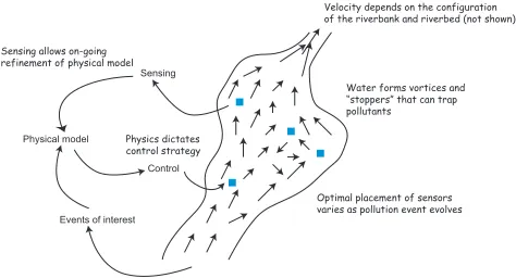
If a node senses a pollutant, the mission goal is to monitor and explore the polluted region. We therefore want to attract more nodes to the area we believe to be polluted. There are various approaches to this. One is to maintain a view of the pollutant density and water behaviour across the network, and condition the movement of nodes according to the gradients observed. Another is to condition the behaviour of nodes according to the flow dynamics of the water, so that (for example) nodes tend to converge on areas down-and up-stream of the initial detection in order to locate the extent of the flow in the preferred direction, and to disperse laterally to determine its extent across the flow (figure 2).

However, there is a countervailing requirement that we do not neglect other areas in pursuit of a single pollution incident: indeed, given that the system is chaotic, we cannot guarantee that the above tactic will take nodes to their optimal placement. We must therefore ensure that not all nodes are attracted to the area, but that some are repelled and continue to conduct surveillance on the rest of the area to detect any other events.

Water forms vortices and “stoppers” that can trap pollutants

Velocity depends on the configuration of the riverbank and riverbed (not shown)

Optimal placement of sensors varies as pollution event evolves

Physical model

Sensing

Control

Events of interest

Sensing allows on-going refinement of physical model

Physics dictates control strategy

Figure 2. Optimal placement of sensors in a river will change according to the flow observed

This is clearly a quite complex set of conditions to meet, especially in the absence of central planning, since we want nodes to behave differently in response to the same stimuli, and to ensure that an appropriate population of nodes exhibits the appropriate behaviour. What wecansay, however, is that it is at least in principle possible to define an optimal placement of nodes, and indeed an optimal dynamics for node movement, for a given pollution scenario in a given water flow. Indeed, for any configuration of nodes, we can define the optimal motion of those nodes to improve their positioning in order to sense a given event. Essentially this means that we define a dynamical system over the sensor system, in which the evolution of the system is defined by the particular tactics we deploy. We can then use the optimal model as a reference against which to evaluate the efficiency of any tactics we employ.

sim-ulate them, we can define optimality against the model we have, and can explore the refinement of sensing tactics within this environment. This has several important conse-quences.

Firstly, any refinement of the environmental model trans-lates directly to our ability to improve our sensing tactics. As we gain a better understanding of the environment, we can refine the physics of water flow and so forth, an use this to influence the tactics we make use of. This refinement can come from observations made by surveying, or from improved computer modelling off-line. Critically, it can also potentially come from the observations made by the nodes themselves, in that the node can compute the difference between what the model says it should observe about water flow in a location and the actual observations it makes. Clearly such refinement is a complex problem and not well-understood, and we are looking to explore this further with domain experts.

Secondly, since our sensing approach is derived directly from the physics of the phenomenon being sensed, we can gain more confidence that the observations we make are representative of the actual situation, in a way that is perhaps less possible with fixed placements or random observations. This claim comes with several caveats, of course, most notably that the chaos in the physical situation makes it possible (indeed, likely) that unexpected situations will occur.

Thirdly, the approach says nothing about the specific tactics or programming model used. This means that any programing model that is deemed promising can be tested against the model, and against other approaches. The model provides both a specification of a “correct” behaviour and a reference against which to test different approaches in a controlled way.

It is important to remember that, although the model is specified globally (in the sense of being a complete description of the area rather than being simply a local view), it is implementation architecture-neutral. Moreover we may be able to use the structure of the model to derive distributed algorithms. Whether we use a physically-inspired approach such as field-base co-ordination [8], a multi-agent systems approach [9], a function of the various vector derivatives of the physical model [4], a policy-based approach, or a more traditional distributed system, the results can still be evaluated and refined within a common framework. Having a physical model may both help in the creation of tactics and in their evaluation and verification.

This neutrality is not universal in the autonomic systems literature, in which problem and solution are often closely tied together. While this can often yield a solution, there must inevitably be concerns that (firstly) the chosen ap-proach will not continue to produce acceptable results if the problem changes, and (secondly) that it can be difficult to see where the problem ends and the solution begins.

Separating means from mechanism encourages a wider and more scientific exploration of the potential solution space. We believe that this is essential at the current state of the art in autonomic sensor systems, since there is no consensus, and only limited real-world experience, in the deployment and evolution of such systems over time. This is not of course to say that emergent properties are a priori undesirable – but nor are they a priori desirable, and the use of emergence should be a tool, and not a assessment criterion, in the development of autonomic systems.

3.5. Generalising the approach

We believe that this approach, of using a physical model to provide a reference against which to evaluate different implementations and tactics, offers significant benefits for exploring the landscape of autonomic control for WSNs. We suggest that the following stages provide a framework for developing such well-founded control models:

1) Obtain or develop a physical model of the phe-nomenon to be sensed and the environment in which the sensing occurs. The model need not be too fine-grained, but should provide sufficient detail to allow the evaluation of different placements and tactics mod-elled at a reasonable (for example GPS) resolution 2) Define the capabilities of the sensor nodes, in terms

of their sensor range, communications range and other capabilities, especially their ability to move. All these capabilities may be constants, but some or all are likely to be functions of the environment to some degree 3) For each configuration of the environment, determine

an “optimal” placement of sensor nodes. Again, the placement need not actually be strictly optimal, but must be as good as one would seek to accomplish with manual management

4) For each actual configuration of sensor nodes, develop tactics that allow the nodes to move towards the opti-mal configuration. These can deploy any appropriate programming approach, but need to be constrained by the capabilities of the nodes and their relationship to the environment

5) Evaluate each tactic by examining, for example, how long it takes to converge to the optimal configuration. This may not actually be useful in practice, since the environment may change faster than any algorithm’s ability to converge, but it still provides information about the responsiveness of different approaches

4. Conclusion

and demonstrate the connections between the environment and the system being used to interact with it.

A focus on individual solution approaches can sometimes not encourage a broadly-based, comparative approach to exploring the solution space. We have suggested a three-stage approach in which we first model the physics of the phenomenon being observed at some level, use this model to derive a dynamic description of the way in which the sensing system should evolve in response to particular conditions, and then treat the resulting dynamical system as both a specification and a reference for evaluating control tactics used within the senor network itself. In some programming regimes the dynamical system may offer insights into the design of tactics; in any case, it is possible to evaluate the quality, correctness and other properties of a solution against a common benchmark.

The scenario we have presented is one in which we have a serious practical interest, and our future work will be devoted to generating a model of a realistic (although simplified) watercourse and the derivation of tactics for sensing within it. We hope to be able to test our ideas in the field over the coming years, and contribute to the accurate sensing and management of valuable resources.

Acknowledgements

This work is partially supported by Science Foundation Ireland under grant numbers 03/CE2/I303-1, “Lero: the Irish Software Engineering Research Centre”, 07/CE/I1147, “Clarity, the Centre for Sensor Web Technologies”, and 04/RPI/1544, “Secure and Predictable Pervasive Comput-ing”.

References

[1] J. Achenbach. Dead zones appear in waters worldwide. The Washington Post, page A02, August 2008.

[2] B. Anderson. The physics of sailing. Physics Today, pages 38–43, February 2008.

[3] N. Bartolini, T. Calamoneri, E. G. Fusco, A. Massini, and S. Silvestri. Autonomous deployment of self-organizing mobile sensors for a complete coverage. In K. A. Hummel and J. Sterbenz, editors,Self-organizing systems, volume 5243 ofLNCS, pages 194–205. Springer-Verlag, 2008.

[4] S. Dobson. An adaptive systems perspective on network calculus, with applications to autonomic control. Interna-tional Journal of Autonomous and Adaptive Communications Systems, 1(3):332–341, 2008.

[5] S. Dobson, S. Denazis, A. Fern´andez, D. Ga¨ıti, E. Ge-lenbe, F. Massacci, P. Nixon, F. Saffre, N. Schmidt, and F. Zambonelli. A survey of autonomic communications.

ACM Transactions on Autonomous and Adaptive Systems, 1(2):223–259, December 2006.

[6] E. Guizzo. Defense contractors snap up submersible robot gliders.IEEE Spectrum, 45(9 (INT)):11–12, September 2008.

[7] J. Kephart and D. Chess. The vision of autonomic computing.

IEEE Computer, 36(1):41–52, January 2003.

[8] M. Mamei and F. Zambonelli. Field-based coordination for pervasive multiagent systems. Springer Verlag, 2005.

[9] G. O’Hare, M. O’Grady, R. Tynan, C. Muldoon, H. Kolar, A. Ruzzelli, D. Diamond, and E. Sweeney. Embedding intelli-gent decision making within complex dynamic environments.

Artificial Intelligence Review, 27(2–3):189–201, August 2009.

[10] D. Pompili, T. Melodia, and I. Akyildiz. Routing algo-rithms for delay-insensitive and delay-sensitive applications in underwater sensor networks. In Proceedings of the 12th ACM Conference on Mobile Computing and Networking, September 2006.