On the epidemic of financial crises

On the Epidemic of Financial Crises

Nikolaos Demiris

Athens University of Economics & Business, Athens, Greece

Theodore Kypraios

University of Nottingham, Nottingham, UK

L. Vanessa Smith

University of Cambridge, Cambridge, UK

June 16, 2013

Abstract

This paper proposes a framework for modelling financial contagion that is based on SIR (Susceptible-Infected-Recovered) transmission models from epidemic theory. This class of models addresses two important features of contagion modelling, which are a common shortcoming of most existing empirical approaches, namely the direct mod-elling of the inherent dependencies involved in the transmission mechanism, and an associated canonical measure of crisis severity. The proposed methodology naturally implies a control mechanism, which is required when evaluating prospective immunisa-tion policies that intend to mitigate the impact of a crisis. It can be implemented not only as a way of learning from past experiences, but also at the onset of a contagious financial crisis. The approach is illustrated on a number of currency crisis episodes, using both historical final outcome and temporal data. The latter require the intro-duction of a novel hierarchical model that we call the Hidden Epidemic Model (HEM), and which embeds the stochastic financial epidemic as a latent process. The empirical results suggest, among other, an increasing trend for global transmission of currency crises over time.

1

Introduction

A financial crisis originating in one country can travel within and beyond its original neigh-bourhood spreading among countries like a contagious disease. Loosely speaking, this phe-nomenon, which was a common feature of the major recent crises, is referred to by economists as ‘contagion’. Contagion by definition can only occur if there are interactions among sub-jects. These interactions can materialise at different levels and through different channels simultaneously, some channels being more important during particular events than others. The literature typically distinguishes between fundamentals-based contagion, a transmission of a crisis from one country to another through real and financial linkages, also known as spillovers, and pure contagion where a crisis might trigger additional crises elsewhere for reasons unexplained by fundamentals. As financial crises spread across countries, they affect nations with apparently healthy fundamentals and sound policies. The better understanding we have of their propagation mechanism, the better we are positioned in proposing policy interventions which can most effectively reduce their contagious spread.

simulation models to investigate the dynamics of financial contagion.

On the empirical front considerable effort has been devoted to documenting the existence of contagion.Various tests have been proposed in the literature for this purpose including among others the Forbes and Rigobon (2002) test based on correlation coefficients and the Pesaran and Pick (2007) threshold test. Dungey et al. (2005a, 2005b) provide a review and comparison of alternative tests of contagion. The bulk of the studies suggest that there is evidence of contagion. For an overview of the empirical evidence of contagion see Dornbusch et al. (2000) and Pericoli and Sbracia (2003). Less emphasis, however, has been placed on modelling the propagation mechanism of financial crises. A class of models that features prominently in the empirical contagion literature is that of cross country probit-type regres-sions of a binary crisis indicator on variables representing potentially important transmission channels. Such channels have been identified as trade links (Glick and Rose, 1999), financial links and the common creditor (Caramazza et al., 2004, and Kaminsky and Reinhart, 2000), neighborhood effects (De Gregorio and Valdes, 2001), and macroeconomic similarities (Sachs et al., 1996). More recently, Dungey and Martin (2007) have proposed capturing financial market linkages during crises through the use of common factors, while Aït-Sahalia et al. (2010) suggest modelling financial contagion using mutually exciting processes.

In this paper we propose a framework for modelling financial contagion which is based on SIR (Susceptible-Infected-Recovered) transmission models from epidemic theory (see for example, Bailey, 1975). This class of models addresses two important features of contagion modelling which are a common shortcoming of most existing empirical approaches, namely the direct modelling of the inherent dependencies involved in the transmission mechanism, and an associated canonical measure of crisis severity. At the same time, it allows to in-corporate features that reflect relevant theoretical and empirical evidence in the literature through the inclusion of appropriate covariates. The proposed methodology naturally implies a control mechanism, which is required when evaluating prospective immunisation policies that intend to mitigate the impact of a crisis. This control mechanism can be implemented not only as a way of learning from past experiences, but also in real-time as a contagious financial crisis unfolds.

episode, the focus is on how crises spread from an initially affected (or ‘infected’) country to the rest of the countries by considering their interaction at the local and global level. We explicitly model regional and global contagious ‘contacts’ and infer the rate of their transmission. These transmission rates allow us to directly quantify the severity of the crisis, in contrast to conventional approaches in the literature where severity is measured by a composite index of macroeconomic indicators, see Kaminsky and Reinhart (1998) and Kaminsky (2006). The methodology also delivers an estimate of the number of countries to financially support in order to prevent a major crisis.

In the proposed framework a country may experience a crisis not only because of its direct links to the originally infected (ground zero) country, but also due to local and/or global contacts with countries that are already infected. Thus, we allow for the so called ‘cascading effect’ following the terminology of Glick and Rose (1999), which is typically ignored in the literature. In fact, the proposed approach effectively considers the set of all possible transmission channels of a crisis. Furthermore, it naturally accounts for an increase in the likelihood of a crisis in a particular country given that there is a crisis elsewhere. This is explored in Eichengreen et al. (1996) and Kaminsky and Reinhart (2000) as being consistent with the existence of contagion.

The methodology is illustrated on a number of currency crisis episodes, using both his-torical final outcome and temporal data. The former provides information on the number of initially ‘healthy’ countries, that were ever affected or otherwise by a particular financial crisis. The information provided by the latter allows to estimate the ‘infection’ and/or ‘re-covery’ times of the crisis, in addition to the trasmission rates. The use of temporal data is necessary for performing real-time analysis of a crisis spread. It requires the introduction of a novel hierarchical model, that we call the Hidden Epidemic Model (HEM), and which embeds the stochastic financial epidemic as a latent process. Our findings, among others, point to an increasing trend for global transmission of currency crises over time.

2

Modelling Framework

Consider the onset of a financial crisis, for example, a currency crisis or a stock market crash, with contagious effects to a given population of, say, countries. Our interest is in modelling the process associated with the propagation of the crisis. The approach can be equally applied to populations of firms or banks, among others.

2.1

The Model

Consider a closed population of N countries, partitioned into regions of varying sizes. Specifically we will assume that the population contains rj regions/groups of size j, where

r=S_j=1rj is the total number of regions and S denotes the size of the largest group. The

total number of countries is then N = S_j=1jrj. The crisis originates in a typically small

number of countries. At the outset, all countries are deemed susceptible to the particular crisis episode. As the crisis unfolds, each country is considered to belong to any one of three states: susceptible, infected (and ‘infectious’) or recovered. Such processes are often referred to as SIR models in epidemic theory. In the SIR model a susceptible country is in a ‘normal’ state and can be affected by the crisis in question. An infective country is in a state of crisis and may trasmit it to other countries. At the end of its infectious period an individual country is considered recovered, in the sense that it plays no further role in the propagation of the crisis. Thus, we effectively assume that a country may not experience multiple recoveries within a single crisis, which appears reasonable for such applications.

A country, say j, remains in crisis for a positive random time, denoted by Ij, which is

allowed to follow any specified distribution. The periods for which the individual countries remain in crisis are assumed to be a-priori independent. While infectious, a country may transmit the crisis to each country within its region at times given by the points of a Poisson process of rate λL. Additionally, each country may trasmit the crisis to any given country

worldwide according to a Poisson process with rate λG/N. That is, there are two levels

of mixing between countries, namely at the local and global level. The contact processes within this construction are assumed to be a-priori independent. This formulation of the model effectively assumes that each country has local contacts with rate λL+λG/N.

no remaining infectious countries in the population. Notice the different scaling of the two transmission rates. This is a common assumption in two-level-mixing models and it implies that there will be more infectious contacts locally if the local population grows, while this is not the case globally.

The model described above is a stochastic epidemic two level mixing model introduced in Ball et al. (1997), where a detailed discussion of related work can be found. While the model does not explicitly assume a latent period for the crisis to unfold once a particular country has been affected, but rather assumes immediate infection, the distribution of the final outcome is invariant to very general assumptions concerning a latent period (see Ball et al., 1997; Andersson and Britton, 2000). The two level mixing model encompasses the so called generalised stochastic epidemic model (GSE), which arises by setting (λL= 0, λG=λ),

that is, assuming all countries mix homogeneously with rateλ.The particular case where the infectious period is exponentially distributed renders the model Markov. As the population size increases, it can be shown (e.g. Ethier and Kurtz 1986) that the solution of this Markov process converges to that of the corresponding system of ODEs known as the deterministic general epidemic.

Epidemic models in their simple deterministic form are not foreign to the economics lit-erature. They typically feature in studies of treatment and control, see for example Geoffard and Philipson (1997), Gersovitz and Hammer (2004) and Toxvaerdy (2010). However, for a complex, highly non-linear phenomenon such as contagion, the stochastic model described above is more appropriate compared to any simple deterministic analog. It is particularly ad-vantageous in that it is suitable for small populations, it can account for the regional/global nature of a crisis, while model complexity and realism can be naturally expanded in different directions, some of which will be discussed below.

Figure 1: Example of a crisis spead over a small population of countries

In the specification described above the population of countries is assumed to represent a complete network i.e. any country can have contacts with any other locally and globally. This is not a restrictive assumption as epidemics upon random networks can be reparameterised to correspond to epidemics on complete graphs (e.g. Neal, 2006, Newman, 2010), and thus can be incorporated into the proposed framework. Furthermore, the population is assumed to be homogeneous, that is, all countries posses similar infectivity and susceptibility properties. This assumption will be relaxed in Section 4.1.1.

Further detail can be added to the model by disaggregating the population according to individual attributes and/or relationship networks based, for example, on economic in-formation. These details can be incorporated through the transmission rates leading to weighted networks. The study of a dynamic process on a weighted network is, essentially, equivalent to the inclusion of a covariate. This can be easily seen by considering the mo-ment generating function of the transmission rate, sayφ(λ), whereφ(λ) = E(exp(−λI)). In the case of a constant infectious period this is simply exp(−λI), the probability of avoiding infection. When information about a particular variable, sayX, becomes available, this can be incorporated using a Cox-type (log-linear) model: λ = λ0exp(αX). Then φ(λ) becomes

φ(λ) = exp[−Iλ0exp(αX)] = wexp(−λ0I) = wφ(λ0). In other words, the inclusion of

2.2

Threshold Parameter

An appealing feature of the proposed modelling framework is that it embodies a threshold parameter which can be utilised as a severity measure of the crisis, thus providing an inherent control mechanism. Stochastic models such as epidemic and branching processes typically generate bimodal realisations where an epidemic may or may not die out quickly, depending on the value of the threshold parameter R0, often referred to as the basic reproduction

number. This is the most important parameter in epidemic theory and is defined as the expected number of infections generated by a typical infective in an infinite susceptible population. Generally, in deterministic epidemic models, R0 is calculated as the largest

eigenvalue of the so called next generation matrix (Diekmann and Heesterbeek, 2000). In the case of a homogeneously mixing stochastic epidemic, it holds that R0 = λE(I),

where λ is the contact rate and I is the infectious period. R0 may be interpreted as a

threshold parameter since its value determines whether or not a major crisis can occur. In particular, if R0 >1 a positive proportion of the infinite population will be affected by the

crisis with positive probability, while if R0 ≤1only a finite number of susceptibles will ever

become infected and thus the crisis spread will swiftly die out. Hence, most control measures aim to reduceR0 below unity. Ball and Donelly (1995) rigorously established the threshold

behaviour of the general stochastic epidemic by coupling the early stages of the epidemic with a suitable branching process.

For the two-level mixing model the threshold parameter, denoted by R∗, is defined in a

similar way to R0. In this case, Ball et al. (1997) couple the epidemic with a branching

process defined on groups. They show that

R∗ =λGE(I)v(λL), (1)

where v(λL)is the average group final size if only local infections are permitted. Specifically,

v(λL) = 1_gS_j=1jµjπj, where µj is the final size within a group of size j, πj = rj/r is the

proportion of groups of sizej andg is the mean group size. It should be noted that whileR∗

is linear in λG, it is nonlinear inλL but linear in v(λL), with the latter being an increasing

function of λL. Details of the calculation of v(λL) can be found in the Supplement.

Most statistical analyses require the assumption of supercriticality, that is R∗ > 1 so

prophylactic measures aim to achieve R∗ ≤ 1, assuming that R∗ > 1 is not desirable while

it also results in underestimating the variability of the model parameters. The inference procedure we will employ does not condition upon R∗ >1.

2.3

Inference Using Final Outcome Data

2.3.1 Final Size Distribution

For a given crisis episode, when only information on the final infected number of countries is available, i.e. final outcome data, it is in principle possible to write down a system of recursive linear equations, the solution of which delivers the probability mass function required for the likelihood. However, solving such a set of equations can be numerically unstable even for small population sizes (see for example Andersson and Britton, 2000, p.18). This problem is greatly amplified for more complex cases like the two level mixing model considered here. The remainder of this section is concerned with the description of an inference procedure that surmounts this complication.

2.3.2 Data and Likelihood

For the two level mixing model, the data are of the form x _{= {xij} where xij denotes the} number of regions containing j initially susceptible countries of which i ever suffered the crisis in question. We will describe a Bayesian inference procedure for the two infection rates λL andλG, given x. By Bayes’ Theorem, the posterior density, π(λL, λG |x), satisfies

π(λL, λG | x)∝ π(x| λL, λG)π(λL, λG), where π(x| λL, λG) denotes the likelihood function

andπ(λL, λG)the joint prior of(λL, λG). The numerical problems mentioned in Section 2.3.1

indicate that the likelihood is analytically and numerically intractable for all but a very small number of countries. We surpass this difficulty by following Demiris and O’Neill (2005a) in augmenting the parameter space using an appropriate random directed graph (digraph) as considered below.

2.3.3 Random Digraph

by Demiris and O’Neill (2005a); see also O’Neill (2009). In short, let each country correspond to a vertex in the random digraph with a directed edge denoting a potential infection. The edges are drawn from vertex j with probability 1− exp(−IjλL) (1−exp(−IjλG/N)) for

local (global) links. It then holds that the distribution of the final outcome of the crisis is equivalent to the distribution of the ‘giant component’ of the graph, that is, the random set of vertices that are connected to the initially affected country (or countries) through directed edges. Additional edges may exist in the digraph, but only the routes emanating from the initially infected can correspond to actual ‘infections’. Flexible models for the infectious periods Ij such as disjoint intervals in real time, representing for example stock

market opening times in the case of a stock market crash, can be easily incorporated into this framework as they only appear through the edge probabilities. To maximise computational efficiency we only consider the graph on ‘infected’ vertices, while all other data contributions are accounted for through the likelihood.

2.3.4 Augmented Likelihood and Posterior

Suppose that the total number of countries that are ever affected by a particular crisis is n=_ijixij, labeled1, . . . , n, and defineGas the random digraph on thesenvertices. For

j = 1, . . . , nletIj denote the infectious period corresponding to vertexjandI = (I1, . . . , In).

We assume that initially there is one known country in crisis, although it is trivial to consider any number of initial infectives, possibly of unknown identity. In fact, it turns out that knowledge of the initial infective is not crucial in the applications to follow.

The augmented posterior density may be written as

π(λL, λG,I, G|x)∝π(x|λL, λG,I, G)π(G|λL, λG,I)π(I)π(λL, λG). (2)

In (2), π(λL, λG) and π(I) denote the priors while the first two terms effectively represent

the augmented likelihood, given by L(x _{| λL, λG,}I_{, G). Provided that G is compatible}

with the data, L(x _{| λL, λG,}I_{, G) is evaluated as the probability of the edges in G times}

the probability of no edges between the n vertices in G and the remaining N −n vertices. Otherwise, L(x_{|λL, λG,}I_{, G)is set to zero.}

LetL

j (Gj ) denote the number of local (global) links emanating from vertexj andNjLthe

with the data. Then the augmented likelihood can be written as

L(x_{|λL, λG,}I_{, G) :=π(}x_{|λL, λG,}I_{, G)π(G|λL, λG,}I_{) =}1_G∼x

n

j=1

{1−exp (−λLIj)}

L j

exp−λLIj

N_jL−L_j

1−exp

−λGIj N

G j

exp

−λGIj(N −

G j )

N

, (3)

where 1_{C denotes the indicator function which takes the value of one when the event C} materialises, and zero otherwise. The MCMC algorithm used to sample from (2) is largely similar to that in Demiris and O’Neill (2005a) where additional details can be found. In brief, standard random walk Metropolis samplers are sufficient for updating the infection rates, while updatingG requires some attention. Specifically,G is a discrete random object with an enormous number of possible configurations, the overwhelming majority of which have negligible posterior probability. Hence, simple strategies like adding and deleting one edge at a time are preferable, as samplers based on more complex proposals can exhibit poor convergence.

3

A Hidden Epidemic Model

Gravelle et al. (2006) and Mandilaras and Bird (2010). However, the focus of these studies is on detecting contagion with the former focusing on changes in volatilities and the latter on correlations across different crisis and non-crisis periods. As such, they do not contain any transmission features associated with the highly complex phenomenon of contagion.

3.1

Model Structure

Consider the observed variableYitfor countryiat timetwherei= 1, . . . , N andt = 1, . . . , T.

LetSitdenote the state of countryiat timet,andEiandRithe times of entry to and recovery

from the crisis. The state variableSit is defined as

Sit =

        

1, t < Ei (susceptible)

2, Ei < t < Ri (infected)

3, t > Ri (recovered).

(4)

For any country i not affected by the crisis Ei = Ri = ∞. Hence, the total final size

l =N_i 1_(E i=∞).

The conditional distribution ofYit|Sitis assumed to follow a Student’stdistribution with

ν degrees of freedom, with mean and variance that depend onSit in the following manner:

Yit|Sit∼

        

tν(µ1, σi1), if Sit = 1,

tν(µ2, σi2), if Sit = 2,

tν(µ3, σi3), if Sit = 3.

The choice of thetdistribution was based on preliminary results of the properties of the tem-poral variable used in the subsequent empirical application. In principle it can be specified as any distribution. We also make the following assumption which characterises the dependence structure of the model:Y1t, Y2t, . . . , YNtconditionally onS1t, S2t, . . . , SNtare independent for

any t, i.e., f(Y1t, Y2t, . . . YNt|S1t, S2t, . . . , SNt) = f(Y1t|S1t)f(Y2t|S2t)· · ·f(YNt|SN t), t =

1, . . . T, where f(·) denotes the density function of a Student’s t distribution. That is, while the state of each country (and thus the log-returns) depends on the state of all other countries in a complex non-linear stochastic manner, conditional upon the state of the coun-try we assume independent variation in the log-return Yit. To capture the inherent

S _{= (Sit, i = 1, . . . , N, t = 1, . . . , T) by the stochastic epidemic two level of mixing model} described in Section 2. As in the standard Hidden Markov Models used in the literature to identify currency crises, see Martinez-Peria (2002) and Brunetti et al. (2008) among others, the above specification can be extended to allow for an autoregressive structure in the mean of the observed series, as well as conditional heteroskedasticity. The latter can be accom-modated by allowing the volatilities to follow, for example, a standard GARCH form. Such extensions will not be pursued here.

3.2

Inference

Without loss of generality we assume that µ = 0, for = 1,2,3 as would be reason-able, for example, in the case of financial (log)return data. We are interested in infer-ring the parameters governing the crisis transmission, and as a by-product the volatilities

σ _{= (σi, i = 1, . . . , N; = 1,2,3) and times of entry to and recovery from the crisis,}

E_{= (E1, . . . , EN) and}R_{= (R1, . . . , RN)respectively.}

Augmented Likelihood

Let Y _{= (Y11, . . . , Y1T;Y21, . . . , Y2T, . . .;YN1, . . . , YNT). The likelihood of the observed data} (Y_{) given the infection rates λG andλL and the volatilities (}σ_{) can be expressed as}

L(Y_{|λG, λL,}σ_{) =}

S

f(Y_,S_{|λG, λL,}σ_)dS_{. (5)}

If the times of entry to and recovery from the crisis for all the countries in the population were known, then parameter estimation would be straightforward. This information, how-ever, is typically not directly observable. In this case, the likelihood given by (5) is intractable due to the requirement of computing the high dimensional integral S(·). To surmount this

problem we augment the parameter space with the sets E _and R_{, and propose a Bayesian} data-augmentation framework for estimation (see, for example, O’Neill and Roberts, 1999). This approach will enable us to treat the times Ei, Ri, i= 1, . . . N as additional parameters

Posterior Distribution

The posterior distribution of the unknown parameters of interest given the observed data and assuming independent priors for λL, λG andσ, is expressed as

π(λG, λL,σ,E,R|Y) ∝ π(Y|E,R,σ, λG, λL)π(E,R|σ, λL, λG)π(σ, λL, λG)

= π(Y_|E_,R_,σ_)π(E_,R_{|λL, λG)π(}σ_{)π(λG)π(λL), (6)}

where π(Y_|E_,R_,σ_{) =}N i=1

T

t=1f(Yit|Sit).

The second term in (6) is the contribution from the epidemic model and following, for example, Jewell et al. (2009) is given by

π(E_,R_{|λL, λG) ∝}

j=k

Mj

× exp

−

T

Ek

i,j

µ_ij(t) dt

× R, (7)

where Mj denotes the (infectious) pressure that an infected country is subjected to just

before it enters the crisis. Thus we have that Mj =_i∈Cµij whereµij is the instantaneous

rate at which countryiexerts (infectious) pressure on countryj just before countryj enters the crisis withµ_ij = λG

N +λL1(i,jin the same region).The setC denotes the set of countries affected

by the crisis at time t. The country that first entered the crisis is labelled by k andT is the time at which the crisis is assumed to be over.

The term R in (7) denotes the contribution of the recovery process to the likelihood of the epidemic model. Assuming independent (random) infectious periods Ii, i = 1, . . . , n,

this contribution is R = n_i=1fI(Ii), where fI(·) denotes the arbitrarily specified

distribu-tion governing the infectious period. The infectious periods are assumed to be distributed according to a Gamma distribution with (hyper) parameters γ and δ (and mean γ/δ), so then R=n_{i=1 Γ(γ)}δγ I_iγ−1exp{−Iiδ}.

Priors

The termsπ(σ_{), π(λG) andπ(λL)denote the prior distributions assigned to the parameters} σ_{, λL and λG respectively. Slowly varying exponential priors are assigned to λL and λG}

prior distributions need to also be assigned to these. An obvious choice for weakly infor-mative priors would be to assume that both parameters are a-priori independent and follow exponential priors similar toλL,λG. As we do not make any assumption about which

coun-try entered the crisis first, we consider a joint prior distribution for k and Ek as follows:

π(k, Ek) = π(Ek|k)π(k) with π(k) = 1/|C| where | · | denotes the cardinality of a set and

π(Ek|k)≡U(−∞, Rk).

3.3

Incorporating Additional Covariates

Explanatory variables are, in principle, straightforward to incorporate within a HEM through the transmission rates. In the most general case one can allow for different covariates affecting local and global rates as follows:

λL,ij =λL0exp(_kαLkXL,ijk), λG,ij =λG0exp(_kαGkXG,ijk),

where λL,ij is the local crisis trasmission rate from the infected country i to the susceptible

country j, λL0 is the local baseline transmission rate, XL,ij = (XL,ij1, ..., XL,ijK) are the

covariates of interest, and α_{L = (αL1, ..., αLK) are the associated coefficients; similarly for}

the global counterparts. An example of a covariate, XL,ijk (XG,ijk) could be the exports

from country i to country j, at the local (global) level or some proxy for financial linkages as will be considered in our empirical application. It is then of interest to infer the effect of the different covariates on the transmission rates by estimating the parametersα_{L and}α_G.

This will allow to evaluate the importance of different channels in the propagation of a crisis across countries. Note that forα_L=α_G=0_{, the baseline hidden epidemic model with two} levels of mixing is recovered. The posterior distribution of interest then becomes

π(λG, λL,αL,αG,σ,E,R|Y) = π(Y|E,R,σ)π(E,R|λL, λG)

× π(σ_{)π(λG)π(λL)π(}α_L)π(α_{G). (8)}

distributions.

Remark 1 Unlike when only final size data are available where the SIR model is invariant to a latent period, this is not true for temporal data. A straightforward extension to consider in

the latter case is a Susceptible-Exposed-Infected-Recovered (SEIR) model which assumes that

once a country enters the crisis state, it can only trasmit the crisis (i.e. become infective)

after a certain time period elapses.

Remark 2 In the case of real-time analysis, the methodology can be extended to conduct inference for the countries more likely to enter the crisis, given the current state of the

process. For this purpose, a trans-dimensional MCMC algorithm (Green, 1995) is required

which accounts for the variable dimension of the parameter space.

Remark 3 A threshold parameter similar to R _{(see Section 2.2) can also be defined for the} hidden epidemic model, taking into account any additional covariate information. In this

case, definitions of typical infective and susceptible countries based upon averaging over their

covariate values could be used for inclusion in the v(λL) term in (1).

4

Empirical Application

variable or combination of variables into the desired indicator. See Jacobs et al. (2005) for a review of the literature on identification of crises.

We begin our analysis by dividing the countries into groups based on geographical loca-tion. A detailed list of the countries and the composition of regions, as well as the countries affected by each of the crisis episodes can be found in Tables A1 and A2 respectively in the Appendix. The regional decomposition is based on the United Nations classification. Alternative population structures such as overlapping groups or networks based on the trade pattern, financial links or macroeconomic similarities between countries could also be consid-ered. Linkages of this type will be incorporated in what follows through the use of covariates as discussed in Section 3.3.

4.1

Final Size Data

In what follows we present posterior summary estimates of the local (λL) and global (λG)

trasmission rates for each of the five currency crisis episodes. Since no information is available in final outcome data regarding the mean length of the period for which a country remains in crisis, we set the infectious period distribution in advance of the data analysis. This should be taken into account when interpreting λL andλG, while R∗ will not be affected as can be

seen from equation (1). In the results that follow, without loss of generality the infectious period is set to unity. Slowly varying exponential distributions with rate 0.01 are used as priors.

The results, summarised in Table 1, give the mean posterior estimates and corresponding 95% credible intervals for the local and global contact rates, as well as the ratio of global (between region) to total (within region) per-country contact rate λG/N

λL+λG/N =

λG

NλL+λG, for each crisis episode. Since the infectious period is set to unity, this ratio also represents the ratio of between to within country-to-country infectious contacts. The results indicate an increase in the global trasmission rate over time across the different currency crises with a simultaneous decrease observed in the local rate. This is particularly apparent from the ratio

λG

literature suggests that currency crises tend to be mostly regional, only a model allowing for both local and global effects can truly assess the relative importance of each of these dimensions in the transmission of crises. However, it must be pointed out that while the 1992 crisis was mainly confined to European countries, the results in Table 1 do not bring out such a feature. Indeed, a further refinement of the analysis is required to shed light on the true nature of the EMS crisis episode. This will be undertaken in Section 4.1.1 where we consider including categorical covariates in the analysis reflecting certain characteristics of the countries involved.

Table 1: Posterior summary estimates for the two-level mixing model

Crisis Episode λL λG _{N λ}λLG+λG

1971 0.445(0.239,0.738) 0.297(0.093,0.618) 0.005(0.001,0.013) 1973 0.349(0.164,0.574) 0.446(0.169,0.868) 0.010(0.003,0.027) 1992 0.018(0.000,0.066) 1.019(0.487,1.731) 0.381(0.073,0.932) 1994 0.013(0.000,0.047) 1.043(0.516,1.777) 0.456(0.102,0.955) 1997 0.011(0.000,0.041) 1.068(0.617,1.616) 0.491(0.127,0.958)

The above results were obtained using the MCMC algorithm described in Section 2.3.4. The computational complexity is mainly determined by the size of the random graph. The small final sizes involved in this application imply highly efficient computations, that is approximate running times of 2-3 minutes per106_{iterations. An additional attractive feature}

of the considered methodology is related to the convergence of the algorithm. Specifically, it is possible to create a measure of approximate monotonicity by considering summary measures of the random graph such as the total number of links. In the case of a homogeneous population (GSE) and constant infectious period the number of links can be thought of as a sufficient statistic; in more general models it is approximately sufficient. Hence, this number can be used as an approximate convergence diagnostic of the MCMC algorithm. For all the reported results we started the algorithm from the two ‘extremes’ in the graph space, that is, a complete graph where all countries have local and global links with all others, and a sparse tree-like graph. Rapid convergence towards the ‘high probability’ region was observed for all the algorithm implementations. This region lies between the two extremes, with the ‘likely’ graphs being of relatively sparse form.

from the digraph. Combined with knowledge relating to the duration of the crisis, this would deliver inference for the time-length of each generation of affected countries. Theoretical bounds for the longest path in the case of a homogeneous random digraph have been derived in Foss and Konstantopoulos (2003).

4.1.1 Multitype Processes

Motivated by the evidence that crises in developing economies are of a different nature than those in developed ones (Kaminsky, 2006), we consider further partitioning our population of countries into developed and developing, based on the world factbook IMF classification. This distinction allows for the possibility of these two groupings having different local and/or global rates, rather than assuming equal susceptibility and infectivity rates across all coun-tries. It therefore enables to distinguish whether a particular crisis episode affected mostly developed and/or developing countries, avoiding potential misjudgement that may arise from overlooking the degree of economic development of the countries under study. In addition, an analysis that considers a population of multiple types can be useful in uncovering impor-tant transmission channels that may go unobserved in the context of a single type model, as will become clear in what follows. This kind of extension essentially involves introducing categorical covariates into our model specification that can be handled using multitype epi-demic models. Table 2 below gives the proportions of the affected developed and developing countries across the different crisis episodes.

Table 2: Proportions of affected countries across the different crisis episodes

Crisis Episodes 1971 1973 1992 1994 1997 Developed 19₂₈ 19₂₈ 10_{29 29}2 ₂₉4 Developing ₁₁₃0 ₁₁₃0 ₁₃₀0 ₁₃₁9 ₁₃₁13

Consider the case of the 1992 EMS crisis where 10 out of 29 developed countries were affected, while no developing country suffered the crisis in question. Moreover, all affected countries were in Europe (see Table A2 in the Appendix) so we would expect a high local transmission rate among developed countries, which could not have been deduced from Table 1.

reflecting the data provided in Table 2. To see this let ΛL = {λij,L} and ΛG = {λij,G},

i, j = 1,2, denote the 2× 2 matrices of local and global infectious rates, respectively. Subscript 1 (2) refers to the developed (developing) countries, so that for example λ12,L

denotes the local rate at which the crisis affecting a developed country is transmitted to a developing country. It is evident that the number of infection rates to be estimated has now increased considerably relative to the single type model. Certain modelling restrictions are therefore necessary for identifiability, unavoidably for the λG’s and possibly for theλL’s

depending on the dataset under consideration, see Britton (1998) and Britton and Becker (2000) for a detailed discussion.

We consider the following restriction: we allow for distinct local rates when the data contain sufficiently rich information for identification purposes. This is not always the case. Based on the data provided in Table 2, for the earlier crises of 1971, 1973 and 1992 no developing countries were affected. Hence, the data contain no information with respect to the local and global transmission of these crises from one developing country to another, that is λ22,L and λ22,G, respectively, and hence results will be largely informed by the prior. In

addition, convergence of the MCMC sampler may be problematic so special care is required in efforts to overcome issues of parameter redundancy. In such cases, for the local rates we assume equal susceptibility and distinct infectivity, which implies λ11,L = λ21,L, and

λ12,L = λ22,L, that is developed countries have different potential in transmitting the crisis

compared to developing ones, while all countries are equally susceptible. Globally, it is well known (e.g. Ball et al., 2004) that at most two transmission rates are identifiable. Thus, in keeping with our local assumptions, we assume common global susceptibility to a crisis, but distinct global infectivity. We consider this choice to be reasonable within the present context. Scenarios with alternative susceptibility levels, potentially defined based on economic information, are also possible. In fact, within our Bayesian framework it is possible to consider any structure for ΛL and ΛG subject to the required identifiability restrictions.

Table 3: Posterior summaries (means and standard deviations) for the two type model with equal local and global vulnerability for each grouping

Crisis Episode ΛL=

λ11,L λ12,L

λ21,L λ22,L

ΛG=

λ11,G λ12,G

λ21,G λ22,G

1971 0.475(0.211) 0.091(0.089) 0.761(0.356) 0.053(0.053) 1973 0.284(0.130) 0.075(0.076) 1.028(0.417) 0.054(0.053) 1992 0.170(0.086) 0.037(0.037) 0.645(0.390) 0.100(0.099) 1994 0.115(0.093) 0.065(0.032) 0.194(0.135) 0.559(0.238) 1997 1.017(0.394) 0.070(0.030) 0.138(0.098) 0.454(0.186)

Note: The matrixΛL(ΛG)contains the local (global) estimated trasmission rates, where subscripts 1 and 2

refer to the developed and developing countries, respectively. Standard deviations are reported in brackets. The restrictionsλ11,L=λ21,L andλ12,L=λ22,L are imposed onΛL,and λ11,G =λ21,G andλ12,G=λ22,G

are imposed onΛG.

Table 4 presents results under distinct local and equal global vulnerability. Results for this case are only reported for the more recent crises, 1994 and 1997, owing to the lack of information in identifying the local transmission rate, λ22,L, as explained earlier. For both

these episodes, allowing for distinct local susceptibility shows that the local transmission of the crisis is largely from developing to developed countries, as would be expected from the ratios reported in Table 2. A reasonably high local transmission rate is also observed between developed countries. Transmission rates at the global level are similar to those reported in Table 3.

Table 4: Posterior summaries (means and standard deviations) for the two type model with distinct local and equal global vulnerability for each grouping

Crisis Episode ΛL=

λ11,L λ12,L

λ21,L λ22,L

ΛG=

λ11,G λ12,G

λ21,G λ22,G

1994 0.299(0.235) 0.264(0.262) 0.191(0.137) 0.567(0.251) 0.657(0.317) 0.070(0.035) 0.191(0.137) 0.567(0.251) 1997 0.366(0.183) 0.189(0.153) 0.147(0.103) 0.450(0.185) 0.924(0.325) 0.064(0.036) 0.147(0.103) 0.450(0.185)

Note: The matrixΛL(ΛG)contains the local (global) estimated trasmission rates, where subscripts 1 and 2

refer to the developed and developing countries, respectively. Standard deviations are reported in brackets. The restrictionsλ11,G=λ21,G andλ12,G=λ22,G are imposed onΛG.

4.2

Temporal Data

As such, we consider daily log changes in nominal exchange rates as our observed data, that can be used to estimate the entry to and exit from the crisis, in addition to the transmission rates and volatility parameter. To capture the well documented importance of trade and financial linkages in the spread of contagious currency crises, we include related variables as covariates in the hidden epidemic model. Since the relative importance of the trasmission rates has already been extensively discussed, our focus will be on assessing the significance of these covariates.

4.2.1 Exchange Rates

We use daily log exchange rate returns for those countries affected by the crisis, for each crisis episode. While in principle exchange rate data should be considered for all countries in the sample, we proceed by making use of the knowledge of those countries that were affected by the crisis for consistency with the analysis in Section 4.1. The Deutsche Mark is used as the reference currency for the 1992 episode, given that this was the anchor currency within the European Monetary System at the time, and the US dollar for the 1994 and 1997 crises. The returns were originally computed over a five year window, including two years preceding and two years following the crisis year. However, to avoid overlapping crises, the final estimation samples were chosen as, 01/01/1990-15/03/1994, 16/03/1994-31/12/1996, and 01/01/1997-13/03/1998 for the 1992, 1994, and 1997 crises, respectively. Further details regarding the data are available in the Supplement. Among the infected countries for the 1994 and 1997 crises, Argentina and Hong Kong maintained an exchange rate peg and were therefore excluded from the sample for the purpose of the HEM analysis.

4.2.2 Covariates

assets from other countries. Countries affected by a crisis rely heavily on borrowings from the common lender. About 10% or more of the common bank liabilities are normally held in an infected country (Caramazza et al. 2004). We consider trade covariates for the 1992, 1994 and 1997 crisis episodes. Financial covariates are considered only for the latter two, due to data non-availability. The crises of the seventies are excluded from the analysis for the same reason.

Trade Covariates Glick and Rose (1999) consider a number of aggregate measures of direct and indirect trade, centered on the ground zero (initial infective) country and focusing exclusively on exports. These and other similar measures are considered in a number of studies, for example Van Rijcheghem and Weder (2001), Dasgupta et al. (2011), and Haile and Pozo (2008), that use probit type models.

We use the disaggregate matrix of bilateral trade relationships between the infected countries and all trading partners directly in our model. To adjust for the varying size of countries in our sample we consider trade shares, constructed as the ratio of bilateral trade between the infected country i and each of its trading partners j within the total trade of country i. Specifically, we consider two sets of trade covariates, one based exclusively on annual export figures from the IMF Direction of Trade Statistics (DOTS) and the other based on the average of import and export figures. The latter allows to assess the importance of imports, which is ignored in the analysis of Glick and Rose (1999) as they admittedly point out.

Both trade covariates are based on annual figures averaged across the three years typically immediately preceding each crisis episode. See the supplement for more details. Countries where data for more than 20% of trading activity were not available were dropped from the sample for each crisis episode. This resulted in sample sizes of 99, 107, 106 countries for the 1992, 1994 and 1997 crises, respectively, for exports only, and 124, 133 and 132, respectively, for imports and exports. For the purpose of sensitivity analysis we further excluded countries where more than 30% of trading activity was not available and the results were very similar. We model the instantaneous rate at which countryiexerts (infectious) pressure on coun-try j, just before country j enters the crisis as µ_ij = λG

N +λL1(i,j in the same region)

×

eαXij, whereX

ij denotes the acting trade covariate, that is the trade share matrix of the

λL, λG denote the local and global transmission rates, respectively. Although in principle

one could use a more general model and allow the covariateXij to separately affect the local

and global rates, as discussed in Section 3.3, we opted for a simpler model in the interest of parsimony. We assign a Gaussian prior with large variance to the parameter α as for all covariate effects in the illustrations that follow.

For a given infected country, the stronger its trade linkages with the other countries the higher the rate of transmitting the crisis to these countries, other things being equal. This interpretation is different from that of Glick and Rose (1999) and other authors who focus on the effect of trade on the probability of a country becoming infected, rather than on the probability of the infected country transmitting the crisis to other countries. In our context, the former probability can be evaluated as a function of the transmission rates and the infectious pressure exerted on that country.

Table 5: Posterior summary estimates for the coefficient of the trade covariates

1992 1994 1997

Imports and Exports Mean 6.19 -30.95 -4.07 Median 6.32 -25.15 -3.02 90% CI (-1.66,13.94) (-74.52,-2.08) (-17.16,5.13)

Exports

Mean 8.51 -48.87 -9.17 Median 8.36 -36.53 -4.76 90% CI (-0.85,18.09) (-125.43,-1.95) (-38.48,5.10)

Financial Covariates Financial covariates for the 1994 and 1997 crises are constructed based on two sets of bi-annual banking data from the Bank of International Settlements (BIS) beginning in 1988, namely international lending from the international consolidated statistics and international borrowing from the locational international banking statistics. As in the case of trade, we constructed three year averages based on those years typically immediately preceding the crisis date. This resulted in 124 and 136 countries for the 1994 and 1997 crisis, respectively. We employ three commonly used measures for financial linkages between the common lender and crisis countries which are described below (see among others Van Rijckeghem and Weder, 2001, Caramazza et al., 2004, Dasgupta et al., 2011 and Haile and Pozo, 2008). USA and Japan are the common lenders for the 1994 and 1997 crises, respectively.

(i) A measure of the importance of the common lender to the crisis country, that is the proportion of borrowing from a common lender, given by F1i = bi,c/bi, where bi,c is total

borrowing of countryi from the common lender candbi is total borrowing of countryi.

(ii) A measure of the importance of an affected country to a common lender, that is the proportion of borrowings of an affected country in the lending portfolio of a common lender, expressed asF2i =li,c/lc,whereli,c is lending of a common lender to countryiandlcis total

lending of a common lender.

(iii) A measure of competition for funds, that is the extent to which country i competes for borrowings from the same common lender as the ground zero country, given by

F Ci =

c

x0,c+xi,c

x0+xi

1−|xi,c−x0,c| xi,c+x0,c

, (9)

the common lender to countyi, andxi is total borrowings of countryi.The higher the value

of F Ci, the greater the competition for funds between countries i and0.

The transmission rate from an ‘infectious’ country i to a ‘susceptible’ country j, µij,

is given by µ_ij = λG

N +λL1(i,j in the same region)

×eαZi, where Z

i denotes the acting

financial covariate eitherF1, F2, or F C, and α the associated coefficient.

Table 6 reports the mean, median and 90% credible interval for the posterior distribution of the coefficient α associated with the different financial covariates, for the 1994 and 1997 crises. These coefficients appear to be largely negative as would be expected. For a given infected country, the greater the proportion of borrowing from a common lender (F1) or in the lending portfolio of a common lender (F2) the more ‘protected’ that country becomes and so the smaller the probability of transmitting the crisis to other countries. The results point to a significant role for the common lender effect in the 1994 crisis, when measured by the F1 covariate.

Table 6: Posterior summary estimates for the coefficient of the various financial covariates

1994 1997

Mean Median 90% CI Mean Median 90% CI F1 -14.14 -13.10 (-30.75,-0.99) -0.72 -0.16 (-8.89,4.94) F2 -15.40 -13.60 (-39.93,4.63) -9.73 -5.91 (-34.33,5.50) FC -7.98 -7.53 (-19.94,2.66) -2.10 -0.35 (-15.71,4.77)

Trade and Financial Covariates Next we consider including both trade and financial covariates together in the model so that we haveµ_ij =λG

N +λL1(i,j in the same region)

×

eα1Xij+α2Zi_{, where X}

ij and Zi denote the acting trade and financial covariates defined as

above, with α1 andα2 being the corresponding effects.

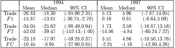
When both trade and financial covariates are included in the model simultaneously, the posterior distributions are wider, as confirmed by the posterior estimates and associated credible intervals presented in Table 7. This table shows the estimates for the posterior distributions of each pair of coefficients,α1 andα2, associated with the corresponding trade

but also as the proportion of borrowings of an affected country in the lending portfolio of the common lender, F2. This result appears to overshadow the significant effect found for the trade channel in the 1994 crisis, when only a trade covariate is included in the model. No significant effect is observed for the 1997 crisis, in line with the earlier findings.

Table 7: Posterior summary estimates for the coefficients associated with the trade and financial covariates

1994 1997

Mean Median 90% CI Mean Median 90% CI Trade -26.83 -18.30 (-85.96,2.35) 5.13 5.96 (-7.87,14.95)

F1 -15.87 -13.81 (-36.75,-2.70) 0.16 0.81 (-6.64,5.09) Trade -34.05 -25.62 (-98.49,0.94) 1.73 3.59 (-16.87,13.16)

F2 -53.03 -39.47 (-152.13,-1.00) -14.56 -4.84 (-60.24,7.22) Trade -23.18 -17.97 (-59.28,0.37) 3.51 4.86 (-10.50,13.76)

F C -10.45 -8.95 (-27.90,0.85) -2.25 -1.16 (-12.80,4.26) Note: Trade refers to the shares of the average of imports and exports.

5

Policy Relevance

Understanding how financial crises spread, through models such as the one proposed here, can enhance in the design and evaluation of immunisation policies to reduce the risks and manage the impact of contagion. So far, at the domestic level, the need for policies aimed at reducing financial fragility has been emphasised; at the international level, the role of better financial standards and of the international lender of last resort has been discussed, see Chang and Majnoni (2001). The latter can provide liquidity to crisis countries to withstand pressures of contagion, as witnessed in the recent economic crises, in the form of rescue packages.

Among the questions increasingly raised on the policy front are how severe is a particular crisis and how to distribute the available resources to sustain countries that have experienced or may be experiencing negative outcomes (how many and which countries to support). The proposed approach can offer answers to such questions, as we illustrate below, by drawing on the past experience of the five currency crises episodes analysed earlier. Lessons from these episodes can offer valuable insight to policy makers for future difficulties.

Sec-tion 2.2 provides a natural formulaSec-tion for evaluating this kind of strategies. In particular, having obtained the parameter estimates of our model, that is the local and global trans-mission rates, we can compute the severity measureR∗ given by (1) for the individual crisis

episodes. Recall that if R∗ > 1 a large number of countries will suffer from the crisis in

question with positive probability, while if R∗ ≤1only a small number of susceptible

coun-tries will ever be affected. Control measures, therefore, typically aim to reduce R∗ below

unity with high probability, which we set to 0.95 in the results that follow. The situation where a major ‘outbreak’ is unlikely to occur is often referred to as ‘herd immunity’. Having computedR∗ we can then sample from its posterior density, and estimate the percentage (or

number) of countries to support, denoted by pv, in order to prevent a major crisis. In other

words, we will estimate the smallest pv such that P(R∗ <1) = 0.95.

We will examine here a simple support strategy where the countries to be supported are chosen uniformly at random. Recall that the threshold parameter without support is given by R∗ = λGE(I)_ν

jjµjπj. When a proportion pv of the countries receives support

the threshold reduces to R∗(pv) = λGE(I)_ν

jjµj

z≥jπr

_z

j

(1−pv)jpzv−j, since the number

of countries prone to the crisis reduces. The percentage pv is computed as the solution to

the equation R∗(pv) = 1. Thus, pv and R∗ are non-linear functionals of the basic model

parameters, at least when the population structure is non-random and known. Inference for this type of functionals has been considered for two level mixing models in Britton and Becker (2000) assuming for simplicity that the outcome within each region is independent of the fate of other regions. Ball et al. (2004) also consider estimating R∗ and pv using

asymptotic arguments and assumingR∗ >1. The methods considered in this paper are free

from these assumptions. Moreover, assuming R∗ > 1 is not particularly satisfactory in our

examples, as will soon become apparent. Alternative support policies, like supporting whole regions chosen at random, are also possible, in which case pv = 1−1/R∗, a well known result

in epidemic theory, see for example Anderson and May (1982), and Ball and Lyne (2006) for the case of structured stochastic models. In the subsequent results we assume that financial support to a country confers complete protection from the crisis, or at least it effectively prevents a particular country from becoming affected.

Table 8 gives estimates of the posterior mean of R∗, P(R∗ < 1) and pv. A graph of the

posterior distribution ofR∗ for all crisis episodes can be found in the supplement. The mean

mean of the 1971 and 1973 crises is 2.19 and 2.95 respectively, while that of the nineties crises is around 1.2. These results corroborate our earlier empirical findings relating to the increasing importance ofλG, which is now reflected in the decreasing length of the 95%

credible intervals forR∗. The corresponding probability of a crisis being subcritical (‘minor’),

given under the headingP(R∗ _{<1), is smaller for the earlier crises compared to the later. In}

accordance, the associated percentage, pv, of countries to support in order to avoid a major

crisis with a 0.95 probability decreases over time as noted by the figures in the last column. The results suggest that the crises of the seventies were of greater severity compared to those of the nineties.

Table 8: Estimated control measures for the various crisis episodes

Crisis Episode R∗ _P(R∗

<1) pv

1971 2.186(0.674,4.610) 0.094 0.291(0.034,0.523) 1973 2.946(0.602,3.632) 0.115 0.265(0.029,0.513) 1992 1.242(0.525,2.425) 0.325 0.240(0.016,0.508) 1994 1.194(0.568,2.170) 0.356 0.230(0.015,0.504) 1997 1.200(0.665,1.938) 0.293 0.210(0.011,0.443)

Note: R∗ _{measures the severity of the crisis, P(R}∗ _{<1) is the probability that only subcritical (‘minor’)}

crises can occur and pvis the critical protection coverage i.e. the percentage of countries to support in order

to avoid a major crisis with a 0.95 probability. Figures in parentheses are the 95% credibles intervals.

The threshold parameter R∗ and associated control measures are also available in the

multitype context, though the calculations are somewhat more involving. In the two type case,R∗ is defined as the largest eigenvalue of a matrixM ={mij}, i, j= 1,2,where, crudely

speaking,m12describes the mean number of contacts from countries of type 1 (developed) to

countries of type 2 (developing). More details regarding the computation of themij elements

can be found in the Supplement.

As demonstrated from the above analysis, the proposed methodology offers a set of valuable control measures that can be used to analyse contagious financial crises. When implemented in real-time, preliminary estimates of the control measures can be computed to evaluate prospective immunisation policies and reduce the countries’ vulnerability to inter-national contagion, see Fraser et al. (2009) for a recent example related to the 2009 influenza pandemic.

6

Discussion

Crises have been a recurrent feature of financial markets for a long time, though it was primarily the crises of the nineties that sparked increased interest in the study of their dynamics and propagation. The experience of the recent crises has rekindled such interest, emphasising the complexity of the financial system, and the need for a better understanding and monitoring of systemic risk and contagious effects.

This paper proposed a modelling framework to analyse financial contagion based on a stochastic epidemic process. The proposed approach directly accounts for the inherent dependencies involved in the propagation of financial crises. In particular, it allows for local and global transmissions through direct and indirect links to the originally affected country. Perhaps more importantly, the framework provides an implicit control mechanism, which includes a canonical measure of the crisis severity along with an estimate of the number of countries to financially support, in order to prevent a major crisis.

assessment by simulating 1000 epidemics from the estimated posterior predictive distribution of the stochastic epidemic two level mixing model for each crisis episode. The results showed larger outbreaks for the seventies and smaller epidemics for the nineties, indicating reasonable model fit.

In addition, the suggested framework naturally caters for temporal data, through the use of the proposed novel hidden epidemic model, contrary to the percolation-based approach. From a methodological viewpoint, it also has several appealing features. It dispenses with approximations such as infinite population, independent regions or supercriticality as is often assumed in epidemic modelling. Moreover, the proposed approach enables one to obtain additional information relating to the propagation of a crisis, not discussed thus far. This includes the set of potential infectors and their corresponding probabilities. The estimation of such crisis characteristics will be more precise in the case of temporal data. Inference regarding ‘the most likely path’ of the crisis spread can also be conducted, resulting in a set of the most probable pathways and their corresponding probabilities. Related work is presented in Shah and Zaman (2011). On the control side, an estimated cost can be assigned to each country and the total cost of the crisis in question can be calculated.

inhomo-geneous networks the threshold parameter should be multiplied by E(k2_{)/E(k) where k is}

the degree of connections and E denotes the expectation operator. The E(k2_{)/E(k) factor}

accounts for non-homogeneous contact networks, see Anderson and May (1991) for an early discussion in the context of HIV modelling. In practice, an extension of this kind would only affect the recovery component of the likelihood associated with the hidden epidemic model, while the infection mechanism and subsequently the control mechanism, would remain un-affected. Mathematically this holds true since the spreading mechanism is of second order and its effect on the initial stages of spreading is negligible.

The superposition of poisson contact processes used in this paper may not be entirely appropriate for banking applications since a number of studies show that the degree dis-tribution of the interbank market network follows a power law (see for instance Arinamin-pathy et al., 2012, and references therein). However, it should be noted that by using a non-homogeneously mixing population we do allow for a more realistic (small world-type) topology of the underlying interaction network along which a crisis may spread. As such, the methodology of this paper can be used to conduct inference for a number of related mod-els. For example, there are connections to the work of Arinaminpathy et al. (2012) where a bank’s individual health could be determined by the local transmission rate while their confidence indicator may be thought of as corresponding to the global rate. In addition, the individual banks could be assigned to one of two types: large or small. Alternatively, one could adopt a non-poisson contact process, see Streftaris and Gibson (2012) for recently developed models where alternative renewal processes are used. Allowing for time-varying intensities could further be of interest. These can be accommodated by replacing λIi with

∞

0 λi(t)dtfor ‘suitable’ infectiousness functionsλi(t). Such extensions and variants thereof,

are left for future work.

Acknowledgements

Appendix

Table A.1: List of countries and composition of regions

Northern America Southern Europe Eastern Asia Southern Africa

US† _{Bosnia China Botswana}

Canada† _{Croatia Hong Kong}† _Lesotho

Greenland∗ _Greece† _Japan† _{South Africa}

Central America Italy† _Korea† _Swaziland

Belize FYROM Macao Eastern Africa

Costa Rica Malta† _{Mongolia Ethiopia}

El Salvador Portugal† _{Chinese Taipei}∗∗ _Kenya

Guatemala Slovenia† _{South East Asia Madagascar}

Honduras Spain† _{Cambodia Malawi}

Mexico Yugoslavia Indonesia Mauritius

Nicaragua Eastern Europe Laos Mozambique

Panama Belarus Malaysia Reunion∗

Southern America Bulgaria Myanmar Rwanda

Argentina Czech Republic Philippines Tanzania

Bolivia Hungary Singapore† _Uganda

Brazil Moldova Thailand Zambia

Chile Poland Vietnam Zimbabwe

Colombia Romania Western Asia Western Africa

Ecuador Russia Armenia Benin

French Guiana∗ _{Slovak Republic Azerbaijan Burkina Faso}

Guyana Ukraine Bahrain Gambia

Paraguay Western Europe Cyprus Ghana

Peru Austria† _{Georgia Guinea-Bissau}

Suriname Belgium† _{Iraq Ivory Coast}

Uruguay France† _Israel† _Liberia

Venezuela Germany† _{Jordan Mali}

Caribbean Netherlands† _{Kuwait Mauritania}

Bahamas Switzerland† _{Lebanon Niger}

Barbados Central Asia Oman Nigeria

Dominican Republic Kazakhstan Qatar Senegal Guadeloupe∗ _{Kyrgyzstan Saudi Arabia Sierra Leone}

Haiti Tajikistan Syria Togo

Jamaica Turkmenistan Turkey Middle Africa

Martinique∗ _{Uzbekistan United Arab Emirates Angola}

Trinidad Southern Asia Yemen Cameroon

Northern Europe Afghanistan Northern Africa Central Africa Republic

Denmark† _{Bangladesh Algeria Congo}

Estonia India Egypt Gabon

Finland† _{Iran Libya Guinea}

Iceland† _{Pakistan Morocco Zaire}

Ireland† _{Sri Lanka Sudan Oceania}

Latvia Tunisia Australia†

Lithuania Fiji

Norway† _{New Caledonia}

Sweden† _{New Zealand}†

UK† _{Papua New Guinea}

Notes: The regional decomposition is based on the United Nations classification. † _{denotes countries classified as developed}

based on the world factbook IMF classification, while the rest of the countries belong to the developing group. ∗_and∗∗_denote

Table A.2: Crisis episodes and affected countries

Crisis Year Countries Affected

Break Down of Bretton Woods 1971

US, Denmark, Finland, Ireland, Norway, Sweden, UK, Greece, Italy, Portugal, Spain, Austria, Belgium, France, Germany‡_{, Netherlands,}

Switzerland, Australia, New Zealand

Collapse of the Smithsonian Agreement 1973

US, Denmark, Finland, Iceland, Norway, Sweden, UK, Greece, Italy, Portugal, Austria, Belgium, France, Germany‡_{, Netherlands,}

Switzerland, Japan, Australia, New Zealand

EMS Crisis 1992 Denmark, Finland

‡_{, Ireland, Sweden, UK, Italy,}

Portugal, Spain, Belgium, France

Mexican Meltdown and Tequila Effect 1994

Canada, Mexico‡_{, Argentina, Brazil,}

Peru, Venezuela, Hungary, Hong Kong, Indonesia, Philippines, Thailand

Asian Flu 1997

Mexico, Argentina, Brazil, Czech Republic, Hungary, Poland, Pakistan, Hong Kong, Korea, Taiwan, Indonesia, Malaysia, Philippines, Singapore,Thailand‡_{, Vietnam, South Africa}

Note: ‡ _{Denotes the country where the crisis originated. Czech Republic and Russia Federation are included in the 1971 and}

1973 episodes corresponding to Czechoslovakia and USSR. The following countries: Armenia, Azerbaijan, Belarus, Bosnia, Croa-tia, Estonia, FYROM, Georgia, Kazakhstan, Kyrgyzstan, Latvia, Lithuania, Moldova, Slovak Republic, Slovenia, Tajikistan, Turkmenistan, Ukraine, Uzbekistan, did not exist at the time of the 1971 and 1973 crisis. Slovak Republic did not exist at the time of the 1992 crisis.

Table A.3: Percentage of trade among infected countries for the different crisis episodes

1992 Crisis Infected countries

% of trade among infected countries

1997 Crisis Infected countries

% of trade among infected countries

Denmark 0.42 Mexico 0.03

Finland 0.47 Brazil 0.09

Ireland 0.61 Czech Republic 0.07

Sweden 0.39 Hungary 0.07

UK 0.37 Poland 0.07

Italy 0.36 Pakistan 0.13

Portugal 0.55 Korea 0.15

Spain 0.48 Indonesia 0.23

Belgium 0.40 Malaysia 0.31

France 0.43 Philippines 0.19

1994 Crisis Infected countries

% of trade among infected countries

Singapore Thailand

0.33 0.22

Canada 0.03 Vietnam 0.46

Mexico 0.04 South Africa 0.04

Brazil 0.08 Peru 0.14 Venezuela 0.08 Hungary 0.01 Indonesia 0.04 Philippines 0.05 Thailand 0.04