Theoretical basis and practical aspects of small specimen creep testing

1

Theoretical basis and practical aspects of small specimen creep testing T.H. Hyde, C.J. Hyde and W. Sun

Abstract

Interest in and the application of small specimen creep test techniques is increasing. This is because it is only possible to obtain small samples of material in some situations, e.g., the scoop samples which are removed from in-service components, the heat-affected zones which are created when welds are used to join components, and the desire to produce only small amounts of material in alloy development programs. It is therefore important that the theoretical basis and practical aspects of small specimen creep testing are clearly understood if the best method is to be chosen for any specific application. The objective of this paper is to provide the theoretical basis for each commonly used test method and to provide information related to some of the practical aspects of the various small specimen creep test methods.

1. Introduction

In order to efficiently and economically operate aero engines, electricity generating power plant, chemical plant, etc., it is necessary to subject some components within them to high temperatures and stresses. This results in the degradation of the properties of the materials used to manufacture the components. The degradation is brought about by the creep and creep damage which occurs and by the detrimental temperature and time dependant changes in the microstructure which are produced during operation [1]. It is therefore necessary to assess the state of the materials at regular intervals, for the purpose of determining the remaining life of the components, and in order to optimise the maintenance work which is carried out during planned outages [2].

One method which has been adopted by some operators, to assess the state of the materials, requires the removal of small samples of material during an outage [3]. The amount of material removed must be small enough so as to have a negligible effect on the strength of the component from which it was removed. For example, “scoop samples” may be removed from steam pipes; steam pipe bends etc. without having an effect on the subsequent behaviour of the components [4]. The typical shape and size of a scoop sample is shown in Fig. 1(a) and (b). The equipment used to remove a scoop sample has been described in detail [5].

The usual way in which the creep properties of a material are determined is to perform, so-called, uniaxial creep tests. Standards have been developed [6], which describe how uniaxial creep tests should be performed; Fig.2 shows the shape and dimensions of a typical uniaxial creep test specimen. The gauge-length (GL) and diameter of the GL are, typically, 30 to 50mm and 6 to 10mm, respectively. Clearly, a specimen of this size cannot be removed from a typical scoop sample. Therefore, it has been necessary to develop non-standard specimen types, and test procedures, from which creep data, corresponding to uniaxial creep data, can be inferred [7]. The small specimen types which have been used are conventional sub-size uniaxial test specimens [8], small punch test (SPT) specimens [9], impression creep test (ICT) specimens [10] and small ring test (SRT) specimens [11, 12]. The shapes of the specimens, typical dimensions and schematic diagrams showing the loading arrangements are given in Figs. 3 and 4.

The relative merits of the four small specimen test types, i.e., conventional sub-size, SPT, ICT and SRT specimens are described in Section 2. Some application of each of these test methods are given in Section 3 for P91 steel and a Ni-based super-alloy. Finally, some discussion and conclusions resulting from the work are given in Section 4.

2

2.1 General descriptions of the deformation behaviour 2.1.1 Conventional sub-size uniaxial test specimens

For this specimen type, the extension of the GL is easily converted to the strain

(

ie,

e

=

ext

_GL

)

and the stress is simply related to the applied load and the initial cross-sectional area of the GL

(

_ie

_s

₌

₄

_{F d}

_p

2

)

_{. If necessary, these} “engineering strains and stresses” can be easily converted to “true strains and stresses”, i.e. !"#$%= '( 1 + ! and +"#$%= + 1 + ! . Hence interpretation of the test results is relatively easy. However, by comparing Figs. 1(a) and 3(a), it is clear that the scoop sample can only be used to produce a “bar” with diameter and length dimensions of about 2mm and 12mm, respectively. In order to keep the gauge length and diameter as large as possible, in some cases [8], end pieces have been ion beam welded to the bar removed from the scoop sample. This is a relatively complicated and expensive process and results in a number of issues which must be considered. For example, the welding of the pieces may produce heat-affected-zones within the GL which may significantly change the properties for some materials. Also, if the grain size is comparable with the cross-sectional dimensions, the results may not be representative of the bulk material creep properties. Also, because the gauge length is small (i.e., about 10mm), compared with that of a conventional uniaxial specimen, the sensitivity of the strain measurement will be relatively low.

2.1.2 SPT specimen

The deformation which occurs in a SPT specimen during testing is the most complicated of all of the small specimen types included in this paper. Hence, interpretation of the data obtained from such a test is difficult; at present, there is no generally accepted method for relating the creep data obtained from a SPT with that obtained by conventional creep testing. The deformation which occurs in a SPT involves the interactions between several non-linear processes. A typical displacement,

D

, versus time, t, plot, obtained from a creep SPT carried out on a P91 specimen at 650˚C, with a load of 160N, is shown in Fig.5.

The specimen starts off as a “flat plate” and undergoes large deformation ending up being approximately conical with a part spherical end. Near the final stages of this deformation process the deflection of the centre of the plate is approximately three times the initial plate thickness. As the deformation proceeds the contact area between the specimen and the indenter increases and the frictional contact conditions change. Associated with the large deformation, large strains also occur. It has been estimated [13] that the strains at the edge of contact between the specimen and the indenter,

e

_eq, are related to the central deformation,

D

, via the following relationship:-

2 3

0.17959.

0.09357.

0.0044.

eq

e

=

D

+

D

+

D

(1)

The corresponding approximate membrane stress,

s

_m, is given by

2 3

1.72476.

0.05638

0.17688

m

P

3

Using equation (1) it can be seen that the value of

e

_eqwhen

D

> 1.0mm, is greater than 30%. This is far in excess of the strain which would be experienced in a conventional uniaxial creep test at a time when secondary creep is occurring. Hence, the minimum displacement rate obtained from a SPT is not directly related to the minimum strain rate in a uniaxial creep test.

In addition to the non-linearities described above the relationship between stress and strain for the material behaviour is nonlinear. In its simplest form the material behaviour model often assumed for the purpose of describing the creep behaviour of a material is the Norton equation, i.e.:

n

B

e

=

s

(3)

It is clear from the above that the SPT is a “complex component test” not a “material test” and that an accurate, simple, mechanics-based method, applicable for all materials, for relating SPT data to corresponding uniaxial creep data is unlikely to exist for this specimen. However, one advantage that the SPT method has over the others is that creep failure data for the components is produced. Hence, the potential for obtaining creep rupture data exists.

There is growing experimental and finite element evidence [13, 14] that empirical relationships can be obtained to relate the creep failure data obtained from SPT tests to that of uniaxial creep rupture tests, and the following relationship has been proposed [14], i.e.,

0.2 1.2

3.33

_{s p s o}

m

P

K a

R t

s

-=

(4)

where

s

_mwould produce the same failure time in a uniaxial specimen as P would produce in a SPT. Ks is a material dependant fitting parameter. A draft code of

practice [14] embodies equation (4).

As with conventional sub-size specimens, the “loaded cross-sectional area” must be large enough, in comparison to the grain size, if data corresponding to bulk properties is to be produced.

The sensitivity of the strain measurements obtained using the SPT method can be estimated from equation 1; re-writing equation (1), using only the first term (which is the dominant term) gives:

6

eq

e

»

D

(5)

This implies that the equivalent gauge length (EGL), i.e., the quantity by which the deformation must be divided, in order to convert the displacement to strain, is about 6mm; this is smaller than the EGL, of about 10mm, that could be produced for a conventional sub-size uniaxial specimen machined from a typical scoop sample.

2.1.3 ICT specimen

4

specimen and therefore, provided the deformation is small compared with the indenter width, d, and the specimen thickness, h, the relationship between stress state and the deformation mode will remain relatively constant. This is reinforced by the fact that for small deformations, the reference stress,

s

_ref, and reference multiplier, D, are both constant and do not depend on the deformation which has occurred. The reference stress method is described in Appendix 1.

For the ICT, a relatively simple relationship exists for the displacement rate,

D

, in terms of the specimen load and dimensions, i.e.,

( )

ref

D

e s

D

=

(6)

and

s

_ref

=

h

p

(7)

where

D

=

b

d

(8)

Equation (6) can be re-written in the form:

( )

ref

d

e s

b

D

=

(9)

Therefore, the measured displacement rate,

D

, can be related to the corresponding strain-rate in a uniaxial test carried out at a stress level of

h

p

. For the typical dimensions of a ICT specimen, i.e., b = 10mm, d = 1mm and h = 2.5mm, the

h

and

b

values are 0.43 and 2.18, respectively.

Hence, there is a straight-forward, mechanics-based method available for converting ICT data to corresponding uniaxial creep data.

In order to ensure that bulk material properties are produced from ICT tests, the grain size should be relatively small compared with the area of contact between the indenter and the specimen. The EGL in this case is the value of

b

d

(see equation (9)), which is typically about 2mm. Compared with the EGL values for conventional sub-size uniaxial specimens (i.e., 10mm) and SPT (i.e., 6mm), the ICT has a relatively low value. Hence, more stringent control, compared with the other test types, is required for these tests. A typical output from an ICT is shown in Fig.7.

2.1.4 SRT specimen

5

( )

(

)

v 2

2

,

2

n n n

Bab Pa

Int n a b

I

æ

ö

D

=

_ç

_÷

è

ø

(10)

and

( )

(

)

2 3

2

,

2

n H n n

Bb

Pa

Int n a b

I

æ

ö

D

=

_ç

_÷

è

ø

(11)

where

1 1

n

n A

I

=

ò

y dA

+ (12)

For a rectangular cross-section beam, equation (12) becomes 2 1

2

2

1

2

n n n o

n

d

I

b

n

+

æ ö

=

_{ç ÷}

+

_{è ø}

(13)

The functions

Int

₂ and

Int

₃are given by

q

q

q

q

q

q

q

q

_qp

q

d

)

cos

1

(

)

cos

'

(cos

d

)

cos

1

(

)

'

cos

(cos

)

n

(

Int

2 ' n ' 0 n

2

=

-

ò

-

-

+

ò

-

-

(14)

and

}

{

d

cos

sin

b

a

sin

)

cos

'

(cos

d

cos

sin

b

a

sin

)

'

cos

(cos

)

n

(

Int

2 2 2 ' n 2 2 2 ' 0 n 3

2

q

+

q

q

÷

ø

ö

ç

è

æ

q

q

-q

+

q

q

+

q

÷

ø

ö

ç

è

æ

q

q

-q

=

ò

ò

p q q

-(15)

where

_q

1

is obtained by solving the following equation, i.e.

0

d

)

cos

'

(cos

d

)

'

cos

(cos

)

n

(

Int

2 ' n ' 0 n

1

=

ò

q

-

q

q

-

ò

q

-

q

q

=

p

q q

(16)

From equations (10) and (11) it can be seen that:

(

)

(

)

3 v 2

,

,

H

b

Int n a b

a Int n a b

D

₌

D

(17)

The variation of

D D

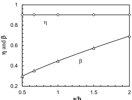
_{H V} with a/b, for a range of n-values, is shown in Fig.9, from which it can be seen that there is a systematic variation of

D D

_{H V} with a/b and that the ratio of

D D

_{H V} is practically independent of n. Using the reference stress method, equation (10) can be written in the form:

6 where

+_#%5= 6 7/

0819 (19)

and

b

is constant for a given a/b.

The variations of

h

and

b

with a/b are shown in Fig.10. It can be seen that

h

is practically independent of a/b.

Rearranging equation (18) gives:

!4 ₊

#%5 = _{./0< 1}:; (20)

Therefore, the data that would be obtained from a SRT (i.e.,

D

_V ), can be converted to the strain rate of a corresponding uniaxial creep test carried out at a stress given by equation (19). The EGL is given by:

4

ab

EGL

d

b

=

(21)

For the particular case of a circular ring,

!4 ₊

#%5 = _.=:9< 1; (22)

where +#%5= 6₀7=

819 (23)

Hence, a mechanics-based method exists for converting SRT data into corresponding uniaxial data.

As with the other test methods, the cross-sectional area should be sufficiently large, by comparison with the grain size of the material, in order to ensure that the results are applicable to bulk material data.

Using typical dimensions for a small ring, i.e., R = 5mm and d = 1mm, equation (21) indicates that an EGL of about 50 is obtained, i.e., the test sensitivity is significantly greater than that of any of the other small specimens; it is comparable to the GL of a conventional uniaxial creep test. This is because the SRT specimen is more “creep compliant” than any of the other specimens and relies upon the accumulation of bending deformation which occurs all around the ring. This is in contrast to the localised deformation which is produced under the indenter of an ICT specimen, for example. Hence, unlike the ICT which requires the indenter material to be orders of magnitude more creep resistant than the specimen material, this is not required for the SRT, i.e., local deformations of the specimen at the contact of the loading pins and the ring, are negligible compared to the deformation resulting from bending.

2.2 Comparison of the different specimen types

7

complexities of the small specimen deformation modes, (ii) the basis of the correlation of the small specimen behaviour and the corresponding uniaxial data, (iii) the sensitivity of the strain measurements (as indicated by the EGL), (iv) the applicability of the results obtained to the corresponding bulk material properties (v) the limitations of the specimen types for some materials and (vi) which test method is the most appropriate for a particular application. Each of these aspects is covered in Sections 2.2.1 to 2.2.5.

2.2.1 Specimen deformation modes

The dimensions of conventional uniaxial material test specimens are such that bulk material properties can be obtained. The test section has a uniform stress and strain state within it, and the specimen is thus a genuine bulk material test specimen. The conventional sub-size uniaxial specimen type is similar in behaviour and is also a genuine material test specimen, but care must be taken to ensure that the result obtained is representative of bulk material behaviour. The next simplest specimen behaviour is that exhibited by the ICT specimen. The stress and strain states are essentially two dimensional, approximating to plane strain conditions. However, unlike the conventional specimen, the stress state in an ICT specimen test is not “uniaxial”. The “slip-line” model, Fig.6 indicates that a combination of compressive and shear deformation exists. However, the deformation is predominantly localised near the indenter and the contact area does not change during the test. In order of complexity, the SRT specimen is next. Except for a region very close to the contact between the ring and the loading pins, the SRT specimen deforms under plane stress conditions. Also, at any particular section, defined by angle,

q

, the loading is predominantly bending and hence at every position, the stress/strain conditions are uniaxial in nature, their magnitudes being related to their distances from the neutral axis. The measured deformation,

D

_V, is related to the accumulated components of bending at every angular position,

q

, and, the load positions are fixed. Therefore, in terms of the stress state, the SRT is similar to the conventional uniaxial specimen test, except the magnitude of the uniaxial stress varies with position throughout the specimen. By far the most complex stress distribution and deformation mode is that within the SPT specimen. The behaviour is essentially axisymmetric, but involves shape change (flat plate to cone), variable contact area, and large strain; other important aspects of the SPT is that the coefficient of friction and clamping force can have a significant effect on the resulting

D

versus t behaviour and on the tf

data.

2.2.2 Basis of the correlation methods

The conventional uniaxial creep test specimen has a uniform stress region and the gauge length and cross-sectional dimensions are large enough to ensure that bulk material properties are obtained. This is achieved by ensuring that the grain sizes (or other metallurgical features) are small compared to the cross-sectional dimensions. Sub-size uniaxial specimens also have a uniform stress region. However, care must be taken to ensure that the grain size is small enough, in comparison with the cross-sectional dimensions, to ensure that “bulk” material properties are obtained. Creep rupture as well as creep strain-rate data can be obtained by using the sub-size uniaxial specimens.

8

derived in this case. However, the approach is of equal accuracy to that used for the correlation of the SRT data, i.e., both are mechanics-based. Both the ICT and SRT correlation methods can be used to obtain creep strain rate data. However, neither would be suitable for determining creep rupture data. Appendix 1 contains descriptions of the inverse reference stress methods used.

The SPT correlation method for obtaining creep rupture data is empirical involving approximate analytical solutions [13, 16, 17], finite element modelling [13, 17] and experimental investigations. Empirical relationships have been obtained which relate the strains at critical positions to the punch displacement, e.g., equation (1); other similar equations have also been derived (e.g. [17]). Also, empirical relationships (e.g. equations (2) and (4)) have been obtained to estimate the stress,

s

_m, which correlates the SPT creep data with corresponding uniaxial creep data. The correlating factor, Ks, is found to be material dependent.

2.2.3 Sensitivity of “strain measurements”

The sensitivity of the “strain measurements” can be conveniently characterised by the magnitude of the equivalent gauge length (EGL). Typical small specimen dimensions and the corresponding EGL values are summarised in Table 1. It can be seen that the sensitivities of the SPT and ICT strain measurements are approximately 8 and 25 times, respectively, worse when compared with the sensitivity of conventional uniaxial creep test specimens. However, the sensitivities of the SRT and conventional uniaxial creep test methods are very similar.

2.2.4 Ability to produce “bulk” material properties

Apart from the “qualitative” rule of thumb often used to ensure that there are sufficient grains on the cross-section of a uniaxial creep test specimen (conventional or sub-size) to produce “bulk” material properties, there is no similar generally accepted method for other specimen types. Even though there is a rule which can be used for uniaxial creep tests, it is not generally accepted what the number of grains on a cross-section should be and the number chosen is usually likely to be far greater than is actually required. Attempts have been made to produce a “quantitative” measure for cross-sectional dimensions [7], but these indicate that as currently used, the rule is too restrictive.

A comparison of the “loaded area” of the various small specimen test types and the conventional uniaxial creep test specimen, with typical dimensions, is given in Table 1. It can be seen that the sub-size conventional specimen, the SPT and the SRT have cross-sectional areas of 3mm2_{, 2mm}2 _{and 4mm}2_{, respectively. The ICT}

specimen has a significantly higher loaded area (i.e., 10mm2_{), which is}

significantly larger than that of the sub-size conventional uniaxial test specimen and is not much smaller than that which would be acceptable for use in a conventional uniaxial creep test specimen.

Unlike the conventional and sub-size conventional test specimen, the SPT, ICT and SRT specimens do not have uniform states of stress within their test sections. Therefore, it is suggested that a better measure of whether the specimens are likely to produce “bulk” material properties is to compare the volumes of material contributing to the specimen deformation; Table 1 includes estimates of the volumes of material contributing to the deformation. It can be seen that the sub-size conventional specimen, the SPT and the ICT have “contributing volumes” of about 30mm3_{, 6mm}3 _{and 10mm}3_{, respectively. The SRT has a “contributing}

volume” of about 120mm3_{, which is significantly higher than the “contributing}

9

the test specimens. It can be seen that the whole volume of the SRT specimen contributes to the deformation obtained in the test. For all of the other test specimens, the vast majority of the specimen volume does not contribute to the deformation obtained in the test.

2.2.5 Practical aspects and limitations

The practical limitations of small specimen creep testing relate to:

(i) The identification of the regions (e.g. HAZ [18] or pipe surface [19]) and the accessibility of these regions in order to remove a material sample; this is a relatively expensive process because it is time-consuming and because experience of using some of the necessary equipment (e.g. to obtain scoop samples) is not widespread and relatively few test facilities exist.

(ii) The manufacture of the test specimens from the material samples; a conventional test specimen (see Fig.2) is complicated involving, in general, turning of plain sections and threads, and grinding and polishing of the gauge section. By comparison, the ICT, SPT and SRT (Figs 3 and 4) are relatively easy to manufacture, using, for example, spark erosion, grinding and polishing processes. The sub-size uniaxial specimen, however, is relatively flimsy and is the most complicated to manufacture, involving all of the processes used for a conventional uniaxial specimen with the added need to electron beam weld the end-pieces onto the test section.

(iii) The complexity of the test equipment; in general, creep tests are carried out under constant load conditions and either dead-weight or servo-electric (or servo-hydraulic) loading methods can be used (the authors have a preference for servo-electric test equipment because the effects of frictional contacts in linear bearings, temperature fluctuations etc. can be eliminated). Schematic diagrams of the loading arrangements are shown in Figs 3 and 4 and drawings and photographs of them are given in Fig 11. Load-line displacements can be measured using extensometry of the type shown in Fig 11 [20] and LVDTs. The choice of extensometry and transducers is not of critical importance but control of the temperature inside the furnace and within the laboratory is of particular importance, especially for those specimens which have small EGLs. Water cooling of the extensometer legs, for example, can be helpful in these cases. Alignment of specimens is important. For the ICT specimens, the contacting surfaces should be flat and parallel and the indenters should be re-ground at regular intervals. For the SPT specimens, the sphere or spherical-ended indenter should be concentric with the outer unclamped diameter of the specimen; care should be taken not to over-tighten the clamped region of the specimen. For the circular SRT specimen the inner surface should be parallel with the axis of the ring and hence the specimen will self-align itself when hung on the upper pin of the fork-end arrangement; greater care would be needed if initially elliptical SRT specimens were to be used.

10

the other specimen types and the load levels are similar to those of the ICT specimens (see Table 2). However, as explained in Section 2.2.2 there is, as yet, no generally accepted method for converting the SPT results to those of a corresponding uniaxial creep test.

2.2.6 Choice of test method for a particular application

The most appropriate small specimen creep test method to use depends on:

(i) The type of creep data required, e.g. the minimum creep strain rate,

e

_min, data or creep rupture, tf data for the corresponding uniaxial creep test,

(ii) The material to be tested, (iii) The test conditions,

(iv) The availability of proof that the “correlation method” can give accurate results.

Table 1 includes a summary of the applicability of each specimen type for determining

e

_minand tf as well as material limitation (if any) for each specimen

type. The standard and sub-size uniaxial creep test specimens can be used to obtain creep curves (including

e

_minand tf data) with the only limitations being due

to the question of whether bulk properties can be obtained with the sub-size specimen and when significant oxidation of the specimen surfaces will occur. If oxidation is a problem, then tests could be carried out in either a vacuum or an “inert” atmosphere. The ICT specimen cannot be used to obtain creep rupture data, but can be used to obtain minimum creep strain rate,

e

_min, data. However, if the material to be tested is such that an indenter material with sufficient creep strength (i.e., 2 to 3 orders of magnitude more creep resistant than the test material) is not available, then the method cannot be used. Similar limitations to the uniaxial specimen tests may occur for the ICT if surface oxidation occurs. Like the ICT specimen, the SRT specimen can be used to obtain

e

_mindata but not tf

data. However, because the deformation of a SRT specimen does not include a significant component due to the local “indentation” at the contact between the ring and the loading pin, the method can be used to obtain

e

_minfor any material. Oxidation may be a problem if the temperature is too high, in which case it may be necessary to test in a controlled environment. The SPT method has the same limitations as regards oxidation, but in addition, research is continuing to develop methods to convert SPT data to corresponding uniaxial creep data. In the absence of mechanics based conversion methods, empirical methods have been developed and are being used and are included in the draft code of practice for the use of SPT methods [14].

3. Applications of small specimen creep testing methods 3.1 Minimum creep strain rate data

11

the small specimen test results and uniaxial creep strain data can be obtained, as indicated by the results presented in Figs 12(a) and 12(b) using the impression creep test method and in Figs 13(a) and 13(b) using the small ring test method. The test conditions for all of the results presented are such that any oxidation or deformation (causing significant change of shape) would have a negligible effect. Also, except in the case of the Ni-base super-alloy, the uniaxial specimens and small test specimens were machined from adjacent positions in the component. For the Ni-base super-alloy (Fig 13(b)), the small ring test specimen was machined from the component of interest and the uniaxial data was obtained from published data from different sources [22] and this is considered to be the main reason for the slightly worse correlation of the data presented for the Ni-base super-alloy.

3.2 Creep rupture data

The only main advantage which the small punch test method has over the other small specimen test methods is that if the specimen test is left long enough the specimen will finally fracture. Empirical formulae, e.g. equation (4), have been devised in order to correlate the creep rupture data from uniaxial tests with that from small punch tests. The factor, Ks, is material dependent and in the absence of any

further information, it is usually taken to be unity [23].

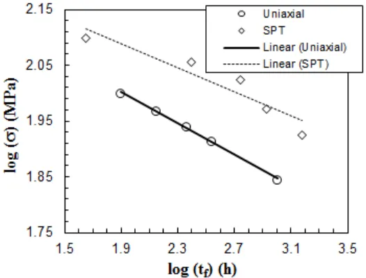
The agreement between the small punch specimen creep rupture data and the corresponding uniaxial data for P91 steel [22] is given in Fig. 14(a). It can be seen that the gradients of the two sets of data (plotted with log-log scales) are similar. The gradient from the uniaxial data is the χ-value in the uniaxial model often assumed, i.e. x

s

t

₌

M

s

- _{. The agreement between the uniaxial and small specimen}

data can be improved by appropriate choice of Ks, as shown in Fig. 14(b).

The SPT method is currently being used by the authors to estimate the creep rupture properties of turbine blade coating materials produced by HVOF [24] and the method seems to be producing good results; this work will be reported in detail [24].

4. Discussion

SPT and ICT methods have been used in earnest for more than a decade and test methods and data processing are at an advanced stage of being accepted. The interpretation method for the ICT is mechanics-based (using an inverse reference stress approach), while the interpretation method for the SPT is empirical. The less well-known SRT method also has a mechanics-based interpretation method.

Small sample extraction methods and specimen manufacture from the samples are relatively straightforward processes and the costs of specimen production and testing should not be prohibitively high by comparison with conventional tests performed on standard uniaxial specimens.

12

13 Table 1.

Specimen Typical dimensions

(Fig.3) Reference Stress EGL (sensitivity) X-sectional Area

(mm2₎ Volume _{contributing to}

definition

(mm3₎

Useful for

ss

e

data

Useful for

tf data

Test material limitation

Volume of specimen

(mm3₎

Conventional Uniaxial Test Specimen

GL = 50mm X-Sectional

Area

»

(

p

d

2

4

)

! "#$

4

50 20-100 600-5000 ü ü X

2000-15000

Conventional sub-size, uniaxial test specimen

GL = 10mm

X-sectional Area

»

2

4

d

p

æ

ö

ç

÷

è

ø

! "#$ 4

10 3 30 ü ü X 100

SPT d = 8mm

ap = 2mm

Rs = 1.25mm

to = 0.5mm

~ '(

$_!

3.33+,-.$./

6 2 6 ? ? X 25

ICT b = 10mm

d = 1mm h = 2.5mm

0 !

12#2

2 10 10 ü X ü 250

SRT R = 5mm

d = 1mm

bo = 2mm _o 2

PR

b d

h

(η = 0.892)

25 2

4

R

d

b

æ

ö

ç

÷

è

ø

(β = 0.448)

2 x 2 (= 4)

[image:13.842.69.537.439.481.2]

120 ü X X 120

Table 2. Loads required (for specimens with typical dimensions) to produce conditions corresponding to a uniaxial stress of 100MPa.

Specimen Conventional

uniaxial creep test specimen

Sub-size uniaxial creep test specimen

ICT specimen SPT specimen SRT

specimen

14

References

1. Tvergaard, V. Creep failure by degradation of the microstructure and grain boundary cavitation in a tensile test. Acta Metallurgica, Volume 35, Issue 4, Pages 723-933, 1987.

2. Sun, W. and Hyde, T.H. Power plant remaining life assessment using small specimen

testing techniques. 9th _{Annual Conf. on Operational Outages for Power Generation.}

28-30 March 2011, Amsterdam, The Netherlands.

3. Parker, J.D. and Purmensky, J. Assessment of performance by monitoring in service

changes in material properties, 9th _{Euro. Conf. on Fracture, Reliability and Structural}

Integrity of Advanced Materials, Varna, 1992.

4. Hyde, T.H., Sun W. and Brett, S.J. Some recommendations on standardization of impression creep testing. Proc. of ECCC Conf. on Creep and Fracture in High Temperature Components - Design and Life Assessment, April 2009, Dübendorf, Switzerland, pp. 1079-1087.

5. Anderson, R. Summary of Rolls-Royce material sampling capabilities with potential relevance for subsequent creep analysis programmes. Practitioner's Meeting on Impression and Other Small Specimen Creep Testing. Nottingham. 8 March 2011.

6. Uniaxial creep testing in tension - Method of test. ISO 204: 2009. Metallic material.

7. Hyde, T.H., Sun, W. and Williams, J.A. The requirements for and the use of miniature test specimens to provide mechanical and creep properties of materials: - a review. International Materials Reviews 52 (4), 213-255, 2007.

8. Askins M.C. and Marchant K.D. Estimating the remnant life of boiler pressure parts, EPRI Contract RP2253-1, Part 2, Miniature specimen creep testing in tension, CEGB Report., TPRD/3099/R86, CEGB, UK, 1987.

9. Parker, J.D. and James, J.D. Creep behaviour of miniature disc specimens of low alloy steel, ASME, PVP 279, Developments in a Progressing Technology, 167-172, 1994.

10. Hyde, T.H., Sun, W. and Becker, A.A. Analysis of the impression creep test method using a rectangular indenter for determining the creep properties in welds, Int. J. Mech. Sci., 38, 1089-1102. 1996.

11. Hyde, T.H. and Sun, W. A novel, high sensitivity, small specimen creep test. J. of Strain Analysis 44 (3), 171-185, 2009.

12. Sun, W. and Hyde, T. H. Determination of secondary creep properties using a small ring creep test technique. Metallurgical Journal, Vol. LXIII, 185-193, 2010.

13. Li Y. Z. and Šturm R. (2008) Determination of creep properties from small punch

test. Proc. ASME Pressure Vessels and Piping Division Conference. July 27-31, 2008, Chicago, Illinois, USA.

15

15. MacKenzie, A.C. On the use of a single uniaxial test to estimate deformation rates in some structures undergoing creep, Int. J. Mech. Sci. 10, 441-453, 1968.

16. Yang Z. and Wang Z-W. (2003). Relationship between strain and central deflection in small punch creep specimens. Int. J. Press. Vess. & Piping 80, 397-404.

17. Hyde, T. H., Miroslav, S., Sun, W. and Hyde C. (2010). On the interpretation of results from small punch creep test. J. of Strain Analysis 45 (3), 141-164, 2010.

18. Hyde, T.H., Sun, W. and Brett S. J. Application of impression creep test data for the assessment of service-exposed power plant components. Metallurgical Journal, Vol. LXIII, 138-145, 2010.

19. Brett, S.J. UK Experience with modified 9Cr (Grade 91) steel, Baltica VII: Int. Conf. on Life Management & Maintenance for Power Plants, Helsinki-Stockholm-Helsinki, p. 48-60, 2007.

20. Hyde, T.H., Sun, W. and Hyde, C.J. An overview of small specimen creep testing. IUTAM Symposium on Advanced Materials Modelling for Structures. 23-27 April 2012, Paris.

21. Hyde, T.H. and Sun, W. Multi-step load impression creep tests for a 1/2CrMoV steel

at 565o _{C, Strain 37, 99-103, 2001.}

22. Hyde, T.H., Hyde, C.J. and Sun, W. A basis for selecting the most appropriate small specimen creep test type. ASME 2012 Pressure Vessel & Piping Conference, Toronto, Canada, 15-19 July, 2012.

23. Sturm, R., Jenjo, M., Ule, B. and Solar, M. Small-punch testing of smart weld

materials, Proc. of the 2nd _{Int. Conf. on Structural Integrity of High Temperature}

Welds, November 2003, IOM3 _{Communications, London, pp. 269-278.}

24 Chen, H., Hyde, T. H., Voisey, K. T., and McCartney, D. G., “Application of small punch creep testing to a thermally sprayed CoNiCrAlY bond coat”, to be submitted to J. Materials at high temperatures.

25. Sun, W., Hyde, T.H. and Brett, S.J. Application of impression creep data in life assessment of power plant materials at high temperatures. J. of Materials: Design and Applications 222, 175-182, 2008.

16

Appendix 1: The reference stress method

For many components made from a material which obeys Norton’s creep law (i.e., !_"=

$%&_{), analytical solutions can be obtained which relate the creep deformation rate to the}

load, component dimensions and material properties (i.e., B and n). For example:-

(i) The tip deflection rate for a tip loaded cantilever beam (see Fig. A1.1) is given

by:

Δ = 2) + 1 2)

& . 2

&-.

) + 2 . /0

1. $. 2/ 310

&

(A1.1)

(ii) The radial deflection rate for an internally pressurised thick cylinder (see Fig

A1.2) is given by:

Δ = 3

2 &-.

. 2 )

&

. 1

56 5₇

0 & − 1

. 56 0

57 . $. 9 &

(A1.2)

(iii) The twist rate for a solid circular bar subjected to a torque (see Fig. A1.3) is

given by:

: = 3 +1

) &

. 3&-.0 _./ 5. $

;

2<5= (A1.3)

It can be seen that, in general, the deformation rates can all be written in the form:-

Δ >? : = A. ) . A0 1BC . $ %&6D & (A1.4)

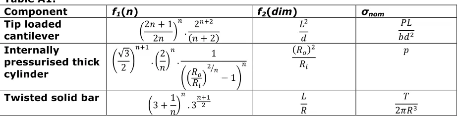
The f1(n), f2(dim) and σnom are summarised in Table A1.

The aim of the reference stress method is to relate the displacement rate to the

creep strain rate, at a so-called, reference stress, σref, via a quantity D, which is, or is

close to being, a constant, i.e.,

Δ = E! %FGH (A1.5)

Using Mackenzie’s method [15], this can be achieved by multiplying the numerator and

denominator of equation A1.4 by a quantity, αn, so that:

Δ =A. )

I& . A0 1BC . $ %&6D & (A1.6)

Hence, α must be chosen to make A_. ) . A₀ 1BC I& _{approximately constant. This can be}

done by substituting two values of n into A_. ) I& _{and equating the resulting expressions,}

such that A. ). I&J = A. )0 I&K. Hence:

I = A. ). A_. )₀

. &JL&K

(A1.7)

17

Δ = E. $ M%&6D &= E! %FGH &

(A1.8)

where,

%FGH= M%&6D (A1.9)

and E =A. ).

M& . A0 1BC (A1.10)

It should be noted that the choice of n1 and n2 is arbitrary, but are best chosen such that

they are in the vicinity of the likely n-value for the material.

The most direct use of the reference stress method is to predict the displacement rate for a component, using equation (A1.8), from the uniaxial creep strain rate obtained

from a test performed with a stress of %_FGH = M%_&6D .

The inverse reference stress approach uses the creep displacement rate

measured in a test in equation (A1.8) to obtain the corresponding “uniaxial” creep strain

rate for a uniaxial stress of σref, i.e.:

! %FGH = Δ

E (A1.11)

It can be seen that the quantity D is the so-called equivalent gauge length (EGL). If an analytical solution cannot be obtained, an alternative approach base on equation (A1.6), can be used. Essentially, a series of finite element analyses with the same geometry (dimensions) and B value are carried out with a range of n values in

order to obtain the variation of Δ ) with n. Hence by plotting Δ ) $ I%_&6D & _{versus n for}

a range of α values the α–value which produces a constant Δ ) $ I%&6D & can be

identified as indicated in Fig A1.4; this value of α is designated as η.

Mackenzie’s method was used to obtain the η and D values for the SRT specimen

and the method illustrated by Fig. A1.4 was used to obtain the η and D values for the

[image:17.595.68.531.487.604.2]

ICT specimen.

Table A1.

Component f1(n) f2(dim) σnom

Tip loaded

cantilever 2) + 1₂₎

& . 2

&-0

) + 2

/0 1

2/ 310

Internally

pressurised thick cylinder

3 2

&-. . 2

) &

. 1

56 57

0 & − 1

&

56 0 57

9

Twisted solid bar

3 +1 )

&

. 3&-.0 /

5

18

Figures

Fig. 1 A typical scoop sample: (a) Dimensions; and (b) A photograph.

Fig. 2 “Standard” uniaxial creep test specimen (GL » 30 – 50mm; dGL » 6 – 10mm; L =

100 – 130mm).

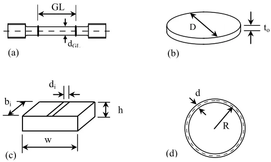
Fig. 3 Shapes and dimensions of small creep test specimens: (a) Conventional sub-size

uniaxial specimen (GL » 5 – 12mm; dGL » 1 – 3mm); (b) SPT specimen (D » 8mm; to»

0.5mm); (c) ICT specimen (w = bi» 10mm; di» 1mm; h » 2.5mm) and (d) SRT (R »

5mm, d » 1mm and depth bo» 2mm).

Fig.

3

Shapes and dimensions of small creep test specimens: (a) Conventional

sub-size uniaxial specimen (GL

»

5 – 12mm; d

GL

»

1 – 3mm); (b) SPT specimen (D

»

8mm; t

o

»

0.5mm); (c) ICT specimen (w = b

i

»

10mm; d

i

»

1mm; h

»

2.5mm) and

(d) SRT (R

»

5mm, d

»

1mm and depth b

o

»

2mm).

(b)

D to

(c) bi

w di

h

(d) d

R (a) dGL

[image:18.595.134.461.113.220.2] [image:18.595.183.411.272.362.2] [image:18.595.171.443.447.610.2]

19

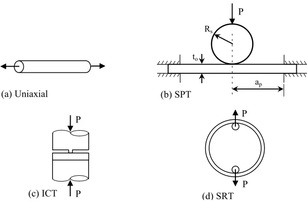
Fig. 4 Schematics diagrams showing the small specimen loading arrangements: (a)

Uniaxial; (b) SPT; (c) ICT and (d) SRT.

Fig. 5 Deformation versus time curve obtained from a SPT for a P91 steel at 650o _{C with}

a load of 160N.

Fig. 6 Approximate “slip-line” model for deformation in an ICT specimen.

Fig.

4

Schematics diagrams showing the small specimen loading arrangements:

(a) Uniaxial; (b) SPT; (c) ICT and (d) SRT.

(a) Uniaxial

(d) SRT P P

(c) ICT P

P

(b) SPT

ap

to

Rs

P

0 0.5 1 1.5 2

0 100 200 300 400 500 600

De

for

m

ation

(m

m

)

Time (hrs)

Fig. 5 Deformation versus time curve obatined from a SPT for a P91 steel at 650

o

_{C with a load of 160N.}

45o

h = 2.5mm

P

[image:19.595.145.460.70.277.2] [image:19.595.182.411.333.513.2] [image:19.595.161.433.554.718.2]

20

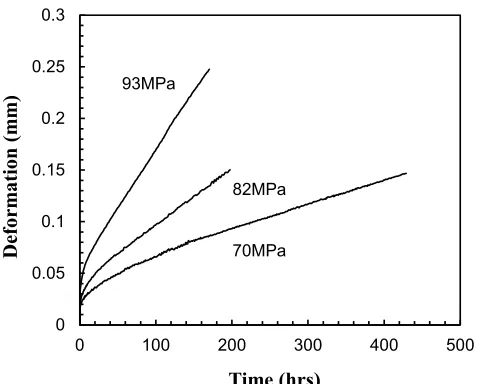
Fig. 7 Typical impression deformation versus time curves for the HAZ material in a P91

weld at 650o _C.

Fig. 8 Bending experienced at position q in an elliptical ring: (a) Dimensions (with a

uniform depth bo); (b) Free body diagram.

Fig. 9 Variations of DH/DV with a/b, for a range of n, for elliptical rings.

0 0.05 0.1 0.15 0.2 0.25 0.3

0 100 200 300 400 500

De

for

m

ation

(m

m

)

Time (hrs)

Fig. 7 Typical impression deformation versus time curves for the HAZ material in a P91 weld at 650o_C. 70MPa

82MPa 93MPa

Fig. 8 Bending experienced at position q in an elliptical ring: (a) Dimensions (with a uniform depth bo); (b) Free body diagram.

b _dq

a d

P/2 Mo q

M (q) P/2 M1

y

x ds

(b)

d

D

,

D

!

a b

P

(a)

0.0 0.5 1.0 1.5 2.0

0.5 1.0 1.5 2.0

D

H

/

D

V

a/b

Fig.

9

Variations of

D

_H

/

D

_V

with a/b, for a range of n, for elliptical rings.

2

[image:20.595.179.418.72.264.2] [image:20.595.126.462.308.440.2] [image:20.595.182.412.496.675.2]

21

Fig. 10 Variation of the η and β parameters with a/b.

0.2 0.4 0.6 0.8 1

0.5 1 1.5 2

h

and

b

a/b

Fig. 10Variation of the hand bparameters with a/b.

[image:21.595.185.411.71.242.2]

22

Fig. 11 Loading arrangements of small specimen test types: (a) SPT; (b) ICT; and (c)

SRT.

Fig. 11 Loading arrangements of small specimen test types: (a)

SPT; (b) ICT; and (c) SRT.

(b)

(c) (a)

Rs

Ball

ap Lower

die Upper

die

Load

[image:22.595.124.471.75.570.2]

23 (a)

(b)

Fig. 12 (a) Correlation of ICT and uniaxial minimum creep strain rate (MSR) data for 316

stainless steel at 600o _{C and 2-1/4Cr1Mo weld metal at 640}o_{C and (b) P91 impression}

MSR data.

Fig. 13(a) Correlation of SRT and uniaxial minimum creep strain rate (MSR) data for a

P91 steel at 650o_C.

1E-6 1E-5 1E-4 1E-3

10 100 1000

M

S

R (

h

-1)

Stress (MPa)

Fig. 12(a) Correlatrion of ICT and uniaxial minimu creep strain rate (MSR) data for 316 stainless steel at 600o_{C and}

2-1/4Cr1Mo weld metal at 640o_C.

Uniaxial (316) Impression (316) Uniaxial (CrMo) Impression (CrMo)

1E-5 1E-4 1E-3

10 100

M

S

R (

1/h

)

Stress (MPa)

Fig. 12(b) Correlatrion of ICT and uniaxial minimu creep strain rate (MSR) data for the P91 steel at 650o_C.

Uniaxial

Impression

-6 -5 -4 -3 -2

1.65 1.75 1.85 1.95 2.05

L

og

(

M

SR)

(

h

-1)

log (s)(MPa)

Fig.

13

(a) Correlation of SRT and uniaxial minumum creep strain rate (MSR) data for a P91 steel at 650

o

_C.

[image:23.595.135.433.71.448.2] [image:23.595.172.423.497.693.2]

24

Fig. 13(b) Correlation of SRT and uniaxial minimum creep strain rate (MSR) data for a

Nickel base super-alloy at 800o_C.

Fig. 14(a) Converted creep rupture data (using Equ. (3), with Ks = 1) obtained from a

[image:24.595.173.421.79.278.2] [image:24.595.165.428.335.535.2]

25

Fig. 14(b) Converted creep rupture data (using Equ. (8), with Ks = 1.275) obtained from

a SPT on a P91 steel at 650o _{C, compared with corresponding uniaxial data.}

Fig. A1.1 A tip-loaded cantilever.

Fig. A1.2 Internally pressurized thick cylinder.

Fig. A1.3 Solid circular bar subjected to a torque T.

Fig.

A1.1

A tip-loaded cantilever.

D

!

d P

b

l

Fig. A1.2 Internally pressurized thick cylinder.

Ro

p

Ri

r

Fig. A1.3 Solid circular bar subjected to a torque T.

q

!

q

g L

R

[image:25.595.165.420.79.279.2] [image:25.595.190.405.327.577.2] [image:25.595.221.376.616.734.2]

26

Fig. A1.4 Variation of

log

[

D

!

(

n

)

/

B

(

as

_nom

)

n

]

with n.

Fig. A1.4 Variation of with n. a5 a4 a2 a1

a3 = h

n

(

)

÷÷ ø ö çç

è æ

as D

n nom) B

[image:26.595.176.423.89.269.2]