warwick.ac.uk/lib-publications
Original citation:Perrone, Valerio, Jenkins, Paul, Spanò, Dario and Teh, Yee Whye (2018) Poisson random
fields for dynamic feature models. Journal of Machine Learning Research, 18 (1). 4626-4670.
Permanent WRAP URL:
http://wrap.warwick.ac.uk/97133
Copyright and reuse:
The Warwick Research Archive Portal (WRAP) makes this work of researchers of the University of Warwick available open access under the following conditions.
This article is made available under the Creative Commons Attribution 4.0 International license (CC BY 4.0) and may be reused according to the conditions of the license. For more
details see: http://creativecommons.org/licenses/by/4.0/
A note on versions:
The version presented in WRAP is the published version, or, version of record, and may be cited as it appears here.
Poisson Random Fields for Dynamic Feature Models
Valerio Perrone* [email protected]
Paul A. Jenkins*† [email protected]
Dario Span`o* [email protected]
*Department of Statistics
†Department of Computer Science
University of Warwick Coventry, CV4 7AL, UK
Yee Whye Teh [email protected]
Department of Statistics University of Oxford Oxford, OX1 3LB, UK
Editor:Lawrence Carin
Abstract
We present the Wright-Fisher Indian buffet process (WF-IBP), a probabilistic model for
time-dependent data assumed to have been generated by an unknown number of latent features. This model is suitable as a prior in Bayesian nonparametric feature allocation models in which the features underlying the observed data exhibit a dependency structure over time. More specifically, we establish a new framework for generating dependent Indian buffet processes, where the Poisson random field model from population genetics is used as a way of constructing dependent beta processes. Inference in the model is complex, and we describe a sophisticated Markov Chain Monte Carlo algorithm for exact posterior simulation. We apply our construction to develop a nonparametric focused topic model for collections of time-stamped text documents and test it on the full corpus of NIPS papers published from 1987 to 2015.
Keywords: Bayesian nonparametrics, Indian buffet process, topic model, Markov chain Monte Carlo, Poisson random field
1. Introduction
The Indian buffet process (IBP) (Griffiths and Ghahramani, 2011) is a distribution for sampling binary matrices with any finite number of rows and an unbounded number of columns, such that rows are exchangeable while columns are independent. It is used as a prior in Bayesian nonparametric models where rows represent objects and columns represent an unbounded array of features. In many settings the prevalence of features exhibits some sort of dependency structure over time and modeling data via a set of independent IBPs may not be appropriate. There has been previous work dedicated to extending the IBP to dependent settings (e.g., Williamson et al., 2010a; Zhou et al., 2011; Miller et al., 2012; Gershman et al., 2015). In this paper we present a novel approach that achieves this by means of a particular time-evolving beta process, which has a number of desirable properties and is better-suited for a different range of applications.
c
For each discrete timet0, . . . , tT at which the data is observed, denote byZt the feature
allocation matrix whose entries are binary random variables such that Zikt = 1 if objecti
possesses featurekat timetand 0 otherwise. Denote byXk(t) the probability thatZikt= 1,
namely the probability that featurekis active at timet, and byX(t) the collection of these probabilities at time t. The idea is to define a prior over the stochastic process {X(t)}t≥0
which governs its evolution in continuous time. In particular, for each feature k, Xk(t)
evolves independently, while features are born and die over time. This is a desirable property in several applications such as in topic modeling, where at some point in time a new topic may be discovered (birth) or forsaken (death). Our model benefits from these properties while retaining a very simple prior where sample paths are continuous and Markovian. Finally, we show that our construction defines a time-dependent beta process from which the two-parameter generalization of the IBP is marginally recovered for every fixed time t
(Ghahramani et al., 2007).
The stochastic process we use is a modification of the so-called Poisson Random Field (PRF), a model widely used in population genetics (e.g., Sawyer and Hartl, 1992; Hartl et al., 1994; Bustamante et al., 2001, 2003; Williamson et al., 2005; Boyko et al., 2008; Gutenkunst et al., 2009; Amei and Sawyer, 2010, 2012). In this setting, new features can arise over time and each of them evolves via an independent Wright-Fisher (W-F) diffusion. The PRF model describes the evolution of feature probabilities within the interval [0,1], allows for flexible boundary behaviours and gives access to several off-the-shelf results from population genetics about quantities of interest, such as the expected lifetime of features or the expected time feature probabilities spend in a given subset of [0,1] (see Ewens, 2004).
We apply the WF-IBP to a topic modeling setting, where a set of time-stamped docu-ments is described using a collection of latent topics whose probabilities evolve over time. The WF-IBP prior allows us to incorporate time dependency into the focused topic model construction described in Williamson et al. (2010b), where the IBP is used as a prior on the topic allocation matrix determining which topics underlie each observed document. As opposed to several existing approaches to topic modeling, which require specifying the total number of topics in the corpus in advance (see for instance Blei et al., 2003), adopting a non-parametric approach saves expensive model selection procedures (such as the one described in Griffiths and Steyvers, 2004). This is also reasonable in view of the fact that the total number of topics in a corpus is expected to grow as new documents accrue. Most existing nonparametric approaches to topic modeling are not designed to capture the evolution of the popularity of topics over time and may thus not be suitable for corpora that span large time periods. On the other hand, existing nonparametric and time-dependent topic models are mostly based on the Hierarchical Dirichlet Process (HDP) (Teh et al., 2006), which implicitly assumes a coupling between the probability of topics and the proportion of words that topics explain within each document. This assumption is undesirable since rare topics may account for a large proportion of words in the few documents in which they appear. Our construction inherits from the static model presented in Williamson et al. (2010b) the advantage of eliminating this coupling. Moreover, it keeps inference straightforward while using an unbounded number of topics and flexibly capturing the evolution of their popularity continuously over time.
novel time-varying feature allocation model. Section 4 describes a fixed-K approximation and an intuitive inference scheme that is built upon in Section 5 to develop an exact MCMC algorithm for posterior inference with the WF-IBP. Section 6 combines the model with a linear-Gaussian likelihood and evaluates it on a range of synthetic data sets. Finally, Section 7 illustrates the application of the WF-IBP to topic modeling and presents results obtained on both synthetic data and on the real-world data set consisting of the full text of papers from the NIPS conferences between the years 1987 and 2015.
2. Background
Before introducing our time-varying feature allocation model we first review its two building blocks, namely the IBP and the PRF. We show how the beta process connects these two models, and we adjust the PRF to develop a time-dependent extension of the two-parameter IBP in the next section.
2.1 The beta and Indian buffet processes
A completely random measure B over a measurable space (Ω,Σ) is a random measure that assigns independent masses to disjoint subsets of Ω. Any positive completely random measure is uniquely characterized by a certain Levy measure on Ω×R+ (see Kingman,
1967). Denote by c a positive function over Ω (concentration function) and by B0 a fixed
measure on Ω (base measure), and assume the base measure B0 is continuous. A beta
process B∼BP(c, B0) on Ω is a completely random measure uniquely characterized by the Levy measure
ν(dω, dx) =B0(dω)c(ω)x−1(1−x)c(ω)−1dx,
where x ∈ [0,1] and ω ∈ Ω. This completely random measure can be represented via a Poisson process. In order to drawB ∼BP(c, B0), draw a set of points (ωi, xi)∈Ω×[0,1]
from a Poisson point process with base measure ν(dω, dx) and let
B = ∞
X
k=1 xkδωk,
where {ωi} are the atoms of the measure B and {xi} their respective weights. Given a
realization B of a beta process BP(c, αB0) with α > 0, one can obtain a draw from the
IBP (Thibaux and Jordan, 2007). This is done by sampling each row zi, i= 1, . . . , N, of
an allocation matrix Z from a Bernoulli processzi |B ∼BeP(B) defined as
zi= ∞
X
k=1
pikδωk, pik
iid
∼Bernoulli(xk).
Notice that as the location of the atoms is not in fact relevant for constructing the matrix
Z, the IBP depends only on the so-called mass parameter B0(Ω) = α and on c(ω). In the
standard IBP,c(ω) is set to be identically 1, so that the Levy measure of the corresponding one-parameter beta process is
If c(ω) is equal to a constant β we have the two-parameter generalization of the IBP (Thibaux and Jordan, 2007).
2.2 The Wright-Fisher model
The starting point of the PRF is the Wright-Fisher (W-F) model from population genetics (Ewens, 2004), which we briefly summarize here. Consider a finite population of organisms of size G such that i ∈ {0,1, . . . , G} individuals have the mutant version of a gene at generation k, while the rest has the non-mutant variant. Assume that each individual produces an infinite number of gametes such that the gametes yielded by a non-mutant become mutant with probability µG and, conversely, those yielded by a mutant become
non-mutant with probabilityβG. Finally, assume that the next generation ofGindividuals
is formed by simple random sampling from this infinite pool of gametes. The evolution of the numberYG(k) of mutant genes at timekis described by a Markov chain on the discrete space {0, . . . , G}. The transition probability pij of switching from imutants (at timek) to
j mutants (at timek+ 1) is given by the following binomial sampling formula:
pij =
G j
(Ψi)j(1−Ψi)G−j,
Ψi =
i(1−βG) + (G−i)µG
G .
Assume the initial state is YG(0) = y0 and denote the resulting Markov chain by YG = (YG(k))k=1,2,... ∼W-FG(µG, βG). Notice that, ifµG = 0 and/orβG= 0, the states 0 and/or
G are absorbing states that respectively correspond to the extinction and fixation of the mutation.
A continuous-time diffusion limit of the W-F model can be obtained, by rescaling time as t=k/G, and taking G→ ∞. The Markov chain YG(bGtc)/G converges to a diffusion
process on [0,1] (see Ethier and Kurtz, 1986; Sawyer and Hartl, 1992) which obeys the one-dimensional stochastic differential equation
dX(t) =γ(X(t))dt+σ(X(t))dB(t),
where
γ(x) = 1
2[µ(1−x)−βx], (2)
σ(x) =px(1−x), (3)
with some initial stateX(0) =x0, over the time intervalt∈[0, T], with rescaled parameters µ = limG→∞2GµG, β = limG→∞2GβG, and with B(t) denoting a standard Brownian
motion. The terms γ(x) and σ(x) are respectively referred to as the drift term and the diffusion term. Denote the diffusion process asX∼ W-F(µ, β).
As there exists no closed form expression for its transition function, simulating from the W-F diffusion requires non-trivial computational techniques. The method we used is out-lined in Dangerfield et al. (2012), a stochastic Taylor scheme tailored to the W-F diffusion. A novel alternative approach that allows for exact simulation has very recently been pro-posed by Jenkins and Span`o (2017). Finally, note that simulating from the W-F diffusion implies doing so for a given diffusion time unit ∆t. While in population genetics diffusion time is related to the population size, in different applications it can be used to regulate the degree of sample path variance, which is linear in time and equal to Var(x(1−x)∆t).
2.3 The Poisson random field
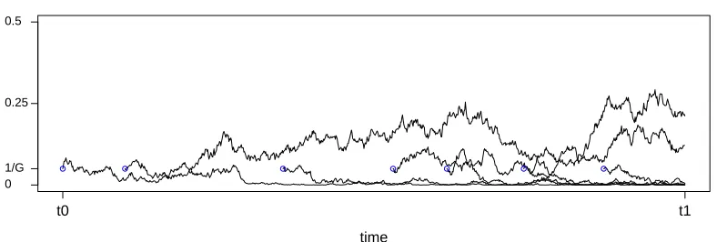
The W-F model describes the evolution of a gene at one particular site. The PRF generalizes it to modeling an infinite collection of sites, each of which evolves independently according to the W-F model. As before, we start with a model with a population of finite size G, before taking the diffusion limit asG→ ∞. For a siteiat which some individuals carry the mutant gene, denote by Xi(k) the fraction of mutants in generation k. Each site evolves
independently according to the W-FG(0,0) model. Further suppose that at each generation
k a number of mutations M ∼ Poisson(νG) arise in new sites with indices j1, j2, . . . jM.
νG is referred to as the immigration parameter of the PRF. Assume that each of the new
mutations occurs at a new site in a single individual, with initial frequency Xjm(k) = 1/G.
Subsequently, each new processXjm(k+ 1), Xjm(k+ 2), . . .evolves independently according
to the W-FG(0,0) model as well (Figure 1). As with pre-existing mutant sites, each process eventually hits one of the boundaries {0,1} and stays there (we say that the mutation is extinct/has been fixed).
Pre−limiting PRF (1 G = 0.05)
time
probability
0 1/G 0.25 0.5
[image:6.612.108.502.441.574.2]t0 t1
Figure 1: Evolution of mutant sites over time in the pre-limiting PRF model. The blue circles indicate mutations arising at a new site.
Consider the limitG→ ∞, so that after the same rescalingt=k/Gof time as in Section 2.2 each site evolves as an independent W-F diffusionXi ∼W-F(0,0). We also assume that
νG → α as G → ∞. This means that in the diffusion time scale the immigration rate is
GνG → ∞, which suggests that the number of sites with mutant genes should explode.
O(G−1) of the newborn processes are not almost immediately absorbed. Therefore, there is a balance between the infinite number of newborn mutations and the infinite number of them going extinct in the first few generations, in such a way that the net immigration rate isO(GνG×G−1) =O(α), and hence the limiting stationary measure is nontrivial. Provided
that we remove from the model all sites whose frequency hits either the boundary 1 or 0, Sawyer and Hartl (1992) prove that the limiting distribution of the fractions of mutants in the interval [0,1] is a Poisson random field with mean density
αx−1dx. (4)
Interestingly, the rate measure of the PRF coincides with the distribution of weights in the one-parameter beta process given in Equation (1). This means that at equilibrium the number of sites whose frequenciesXi(t) are in any given interval (a, b] is Poisson distributed
with rate αRabx−1dx, and these are independent for nonoverlapping intervals. Integrating (4) over [0,1] shows that the number of mutations in the population that has not been fixed or gone extinct is infinite. However, most mutations are present in a very small proportion of the population.
3. Time-Varying Feature Allocation Model
The derivation of the PRF in the previous section shows that, as long as sites reaching frequency 1 or 0 are removed from the model, the equilibrium distribution of the PRF is related to the one-parameter beta process. In this section we generalize the PRF so that it is better adapted to applications in feature allocation modeling. Specifically, we identify mutant sites with features, and identify the proportion of the population having the mutant gene with the probability of the feature occurring in a data observation. The PRF can be then used in a time-varying feature allocation model whereby features arise at some unknown time point, change their probability smoothly according to a W-F diffusion process and eventually die when their probability reaches zero.
3.1 The WF-IBP
Recall from the previous section that mutant sites whose frequency hits 1 are removed from the PRF model. This means that features with high probability of occurrence can be removed from the model instantaneously, which does not make modeling sense. Instead, one expects a feature probability to change smoothly and to be removed from the model only once its probability of occurrence is small. A simple solution to this conundrum is to prevent 1 from being an absorbing state by using instead a W-F(0, β) diffusion with
β > 0. This is a departure from Sawyer and Hartl (1992), due to the differing modeling requirements of genetics versus feature allocation modeling. At the same time, both models let features disappear once their probability gets to 0, which is suitable from a feature allocation perspective and, as we now see, allows for a nontrival equilibrium mean density. We shall denote the modified stochastic process as PRF(α, β). The following theorem derives the equilibrium mean density of PRF(α, β), with proof given in Appendix A:
Theorem 1 The equilibrium mean density of the PRF(α, β) is
In other words, the mean density of the PRF(α, β) is the L´evy measure of the two-parameter beta process, with the immigration rateα identified with the mass parameter, andβ identi-fied with the concentration parameter of the beta process. Whenβ = 1 the one-parameter beta process is recovered. We assume that the initial distribution of PRF(α, β) is its equi-librium distribution, that is, a Poisson random field with mean density (5), so that the marginal distribution of the PRF at any point in time is the same.
We will now make the connection more precise by specifying how a PRF can be used in a time-varying feature allocation model. Denote by Xk(t) the probability of feature
k being active at time t and define our PRF as the stochastic process X := {Xk(t)}.
Assume that at a finite number of time points t = t0, . . . , tT there are Nt objects whose
observable properties depend on a potentially infinite number of latent features. Let Dit
be the observation associated with object i= 1, . . . , Nt at time t=t0, . . . , tT. Consider a
set of random feature allocation matricesZt such that entryZikt is equal to 1 if objectiat
timetpossesses feature k, and 0 otherwise. LetZ :={Zikt}. Finally, letρk be some latent
parameters of feature k and ρ ={ρk} be the set of all feature parameters. Our complete
WF-IBP model is given as follows.
X∼PRF(α, β),
Zikt|X ind
∼ Bernoulli(Xk(t)),
ρk iid
∼H,
Dit|ρ, Zitind∼ F({ρk :Zikt= 1}), (6)
where i= 1, . . . , Nt, t=t0, . . . , tT and k= 1,2, . . .,H is the prior distribution for feature
parameters, and where F(ρ) is the observation model for an object with a set of features with parametersρ.
Since the feature probabilities X have marginal density (5), at each time t the feature allocation matrix Zt has marginal distribution given by the two-parameter Indian buffet
process (Thibaux and Jordan, 2007). Further, since X varies over time, the complete model is a time-varying Indian buffet process feature allocation model. The corresponding De Finetti measure would then be a time-varying beta process. More precisely, this is the measure-valued stochastic process G={G(t)} where
G(t) = ∞
X
k=1
Xk(t)δρk,
which has marginal distribution given by a beta process with parameters α, β and base distribution H. We denote the distribution of G as WFBP(α, β, H). We can also express the feature allocations using random measures as well. In particular, let
Bit= ∞
X
k=1
Ziktδρk
is then
G∼WFBP(α, β, H),
Bit|G∼BeP(G(t)),
Dit |Bit∼F(Bit),
where WFBP denotes our time-varying beta process, and we have usedF(B) to denote the same observation model as before, but with B being a random measure with an atom for each feature, and whose location is the corresponding feature parameter. In the following, we use the notation introduced in (6) instead of in terms of beta and Bernoulli processes for simplicity.
As in the two-parameter IBP,αandβ separately control the distribution of the number of features per object and the total number of features. In addition, the discrete time points
t0, . . . , tT at which the observations are given influence the number of time units for which
the W-F diffusions should be simulated. This introduces a parameter that regulates the strength of the time-dependency or accounts for gaps of varying sizes between successive observations. The time parameter can also be chosen according to the expected life time of features (see Chapter 15 of Karlin and Taylor, 1981). A detailed description of how to simulate from the model is given in Appendix B.
3.2 Related models
The WF-IBP fits a line of research that aims at introducing dependency structures into the IBP. A number of these extensions are designed to drop the exchangeability assumption from the IBP by coupling the rows and columns of the feature allocation matrix, and are thus orthogonal to our work (see Zhou et al., 2011; Miller et al., 2012; Gershman et al., 2015). What we are rather interested in achieving is partial exchangeabilty, whereby objects can be permuted independently at each time point without changing the probability of the process. This is necessary for time-dependent topic models where each time has a different set of documents and there is no correspondence between documents at different times.
IBP and models the dimensionality of the feature allocation matrix and its sparsity inde-pendently.
4. Fixed-K approximation
In order to give more intuition on the exact inference with the WF-IBP that is developed in Section 5, we first describe a finite-dimensional approximation where the number of features is a finite number K, and show that this marginally converges to the WF-IBP asK → ∞. Assume that the random feature allocation matrix Zt has a fixed number of features,
sayK. First, let α, β >0 and consider the beta-binomial model
Zikt | {Xk(t) =xk(t)} iid
∼ Bernoulli(xk(t)),
Xk(t) iid
∼ Beta
αβ K , β
,
∀k = 1, . . . , K,∀i = 1, . . . , Nt. This coincides with the pre-limiting model of the
two-parameter IBP presented in Ghahramani et al. (2007). Then, for each feature, think of the BetaαβK, βdistribution as the stationary distribution of a W-F diffusion with parameters
αβ
K >0 andβ >0. This suggests making the model time-dependent by letting each feature
evolve, starting at stationarity, as an independent W-F diffusion with these parameters. Generate for all times t=t0, . . . , tT the binary variableszikt as
Zikt | {Xk(t) =xk(t)} iid
∼ Bernoulli(xk(t)),
Xk∼WF
αβ K , β
,
∀k = 1, . . . , K,∀i = 1, . . . , Nt. In this way, the closer two time points, the stronger the
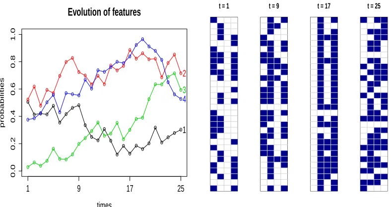
dependency between the probabilities of a given feature (Figure 2). Moreover, as we assume the W-F diffusion to start at stationarity, this construction coincides marginally with the beta-binomial model. The parameters of the W-F diffusion are positive, so that neither fixation nor absorption ever occurs and the number K of features remains constant.
4.1 Fixed-K MCMC inference
Given a set of observations D, a natural inference problem would be to recover the latent feature allocation matrices Z ={Zt}ttT=t0 responsible for generating the observed data, the underlying feature probabilitiesX and their parametersρ. Inference is straightforward; we propose the following updates.
• Z |X, D, ρvia Gibbs sampling.
• ρ|D, Z according to the likelihood model.
• X|Z via Particle Gibbs.
Consider first the Gibbs sampling step to perform posterior inference over the matrices
0.0
0.2
0.4
0.6
0.8
1.0
Evolution of features
times
probabilities
1
2
3
4
1 9 17 25
[image:11.612.111.505.96.305.2]t = 1 t = 9 t = 17 t = 25
Figure 2: Left: underlying feature probabilities over time. Right: corresponding feature allocation matrices. Rows represent objects and columns features, which can be active (blue) or inactive (white).
the components in row i excluding k. We can easily derive for all t the distribution of a given componentZiktconditioning on the state of all other componentsZ−(ik)t, on dataDit,
on the parameters ρ and on the prior probability Xk(t) of feature k. The full conditional
probability of the entryZikt being active is equal to
P(Zikt = 1|Z−(ik)t, Xk(t), Dit, ρ)∝xk(t)P(Dit|Zi−kt, Zikt = 1, ρ). (7)
By the same token, the full conditional probability of the entry Zikt being inactive is
P(Zikt= 0|Z−(ik)t, Xk(t), Dit, ρ)∝(1−xk(t))P(Dit |Zi−kt, Zikt= 0, ρ). (8)
As the matrices Z are conditionally independent given the feature probabilitiesX, equations (7) and (8) can be used to sample the matrices Z independently given the respective feature probabilities at each time. Note that the likelihood P(Dit | Zt, ρ) needs to be specified
according to the problem at hand. A typical choice, detailed in Section 6, is the linear-Gaussian likelihood model, whose parameters can easily be integrated out (Griffiths and Ghahramani, 2011). The updateρ|D, Z over the feature parameters is also specific to the likelihood model and, as we will illustrate, can easily be derived in conjugate models such as the linear-Gaussian one.
Consider now the Particle Gibbs (PG) step (Andrieu et al., 2010) to perform Bayesian inference on the feature trajectories continuously over the interval [t0, tT]. As the prior
probability of each feature is a Beta
αβ
K, β
and the column-wise sums ofZt0are realizations from binomial distributions, by conjugacy we have
Xk(t0)| {Zt0 =zt0} ∼Beta
αβ
K +nkt0, β+Nt0−nkt0
where k = 1, . . . , K, and nkt := PiN=1t zikt denotes the number of objects in matrix Zt
possessing feature k. This posterior distribution can be therefore used to draw the whole set of features at timet0 and the trajectories in the interval [t0, tT] can be obtained via PG.
More precisely, start with an initial reference trajectory xr,kt0:t
T := (x
r,k t0 , . . . , x
r,k tT) for k= 1, . . . , K and, independently for each feature, iterate the following procedure. Draw a given number of particles from the posterior beta distribution at timet0and propagate them forward to time t1 according to WF(αβK, β). At time t1, assign each of these particles and
the reference feature a weight given by the binomial likelihood of seeing that feature active in n(t) objects out of N(t) in Z(t), i.e., xk(t)nkt(1−xk(t))Nt−nkt. Sample the weighted
particles with replacement and propagate the off-springs forward. This corresponds to using a bootstrap filter with multinomial resampling, but other choices to improve on the performance of the sampler can be made (see Andrieu et al., 2010). Repeat this procedure up to timetT and sample only one particle at that time. Reject all the others and keep the
trajectory that led to the sampled particle as the reference trajectory for the next iteration. Notice that the reference feature is kept intact throughout each iteration of the algorithm. This procedure is illustrated more precisely by Algorithm 1, which needs to be iterated independently for each feature to provide posterior samples from their trajectories. To simplify the notation, we drop the index k and write xit|xit0 ∼ WF(αβK, β) for t ∈ [t0, t1] to denote the following: simulate from a W-F diffusion with initial value x(t0) and set X(t1) =x(t1), the value of the diffusion at time t1.
4.2 Approximation for large K
As already noted, the marginal distribution with the fixed-K approximation corresponds to the beta-binomial model, which is the pre-limiting model of the two-parameter IBP. As a consequence, at any fixed time t and as K → ∞, the fixed-K approximation converges to the two-parameter generalization of the IBP, which in turns coincides with the marginal distribution of the WF-IBP. An aspect of interest is then whether the whole dynamics of the fixed-K approximation can be used as a finite approximation of the infinite model in such a way that, the largerK, the better the approximation. Two caveats need to be noted. First, only in the infinite model can features be born. For largeK, however, the number of particles in the fixed-K approximation whose mass is close to zero becomes so large that, with a sufficient amount of time, some of them gain enough mass to become ‘visible’. The behavior of these particles resembles the behavior of the newborn features of the infinite model. Second, as the fixed-Kapproximation has an upwards drift equal toαβ/K, only the infinite model allows for features to be absorbed at 0. This discrepancy is however overcome by the fact that, when K goes to infinity, 0 behaves like an absorbing boundary, in that features get trapped at probabilities close to 0. For these reasons, a comparison of the two models requires relabeling the particles in the finite model in such a way that, whenever a particle goes below a certain threshold≈0, it is considered to have gone extinct, while if its probability is below and later exceedsthe particle is labeled as newborn. We choose this threshold to be= 1/K, as then limK→∞= 0.
Taking these caveats into account, we performed an empirical comparison of the fixed-K
Algorithm 1:Particle Gibbs
Input: Reference trajectory xr
t0:tT;M.
Set xMt0 =xrt0;
Draw xit0 ∼Beta(αβK +nt0,β+Nt0 −nt0) for i= 1, . . . , M −1; Simulate xi
t|xit0 ∼WF(
αβ
K, β) for t∈[t0, t1] fori= 1, . . . , M −1;
Set xMt1 =xrt1;
Compute wit1 = (xit1)nt1(1−xi
t1)
Nt1−nt1 fori= 1, . . . , M;
Sample ¯xit1 withP(¯xit1 =xit1)∝wit1 fori= 1, . . . , M−1; Set ¯xMt1 =xrt1;
Simulate xit|xit1 ∼WF(αβK, β) for t∈[t1, t2] fori= 1, . . . , M −1;
Set j←2;
while tj < tT do
SetxMtj =xrtj;
Computewtij = (xtij)ntj(1−xi tj)
Ntj−ntj
wtij−1 fori= 1, . . . , M; Sample ¯xi
tj withP(¯x
i tj =x
i tj)∝w
i
tj fori= 1, . . . , M −1;
Set ¯xMtj =xrtj;
Simulatexit|x¯itj ∼WF(αβK, β) fort∈[tj, tj+1] fori= 1, . . . , M −1;
Setj←j+ 1;
end
Compute witT = (xtiT)ntT(1−xi
tT)
NtT−ntTwi
tT−1 fori= 1, . . . , M; Sample rnew with P(rnew=i)∝wtiT, where i= 1, . . . , M; Output: New reference trajectoryxrnew
Large−K model (log)
t = 0
t = 1
0 −2 −4 −6
0
−1
−2
−3
−4
−5
−6
−7
Infinite model (log)
t = 0
t = 1
0 −2 −4 −6
0
−1
−2
−3
−4
−5
−6
[image:14.612.165.433.97.285.2]−7
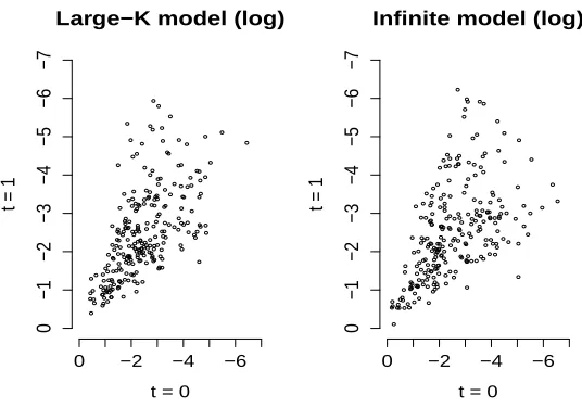
Figure 3: Scatterplot of the log feature probabilities greater than 1/K at time t0 = 0 and at timet1 = 1 to compare the fixed-K (K= 1000) and infinite model.
infinite model. Separately for each model, we took 1000 samples of the feature probabilities at time 0 and at time 1, excluding the ones below 1/K. Figure 3 shows the logarithm of these values for the two models, suggesting a remarkable similarity between the two underlying joint distributions. The validity of this comparison is supported by the maximum mean discrepancy (mmd) test (Gretton et al., 2006), which does not reject the null hypothesis of the two joint distributions being the same. Although this suggests a strong similarity between the dynamics of the fixed-K approximation and the infinite model, we leave a proof of the convergence of these joint distributions as K→ ∞ for future work.
5. Exact MCMC inference
Building on the fixed-K approximation, we now develop a sophisticated MCMC algorithm for exact inference with the WF-IBP. The first point to notice is that, while in the fixed-K
approximation the total number of features is constant over time and equal to K, in the WF-IBP model this is not a finite number. In order to use the WF-IBP for inference it is necessary to augment the state space with the features that are not seen in the feature allocation matrices, but simulating the dynamics of the PRF would require generating an infinite number of features, which is clearly unfeasible. One way to deal with this could be to resort to some sort of truncation, considering only features whose probability is greater than a given threshold and are likely to be seen in the data. We rather choose this truncation level adaptively by introducing a collection of slice variables {St}Tt=1t and adopting conditional
slice sampling (Walker, 2007; Teh et al., 2007). This scheme, which is detailed in Section 5.1, has the advantage of making inference tractable without introducing approximations.
Partition the set of features into two subsets, one containing the features that have been seen at least once among times t = t0, . . . , tT, and the other containing the features that
features cannot be identified individually based on the matrices Z, and as all features are conditionally independent givenZ, we consider seen and unseen features separately. As for the seen features, we use the same Particle Gibbs scheme as in the fixed-K approximation. As for the unseen features, we simulate them via a thinning scheme. The exact MCMC inference scheme can be then summarized by the following updates.
• Z |X, S, D, ρ via Gibbs sampling.
• S|Z, X via slice sampling.
• ρ|D, Z according to the likelihood model.
• Xseen |Z via Particle Gibbs.
• Xunseen |S via thinning.
We present each of these steps in Sections 5.1 and 5.2, which build on the simpler inference scheme developed in Section 4.
5.1 Gibbs and slice sampling
The first step is to augment the parameter space with a set of slice variables. Given the feature allocation matrices Zt at times t = t0, . . . , tT, draw a slice variable St ∼
Uniform[0, xmin(Zt)] for each time t, where xmin(Zt) is the minimum among the
proba-bilities of the features seen in the feature matrixZt. In this way, when conditioning on the
value st of the slice variable, we have a truncation level st and only need to sample the
finite number of features whose probability is above this threshold (Teh et al., 2007). In other words, for all t=t0, . . . , tT, we only need to update the columns of Zt whose
corre-sponding feature probabilityxk(t) is greater than or equal to the slice variablest(note that
these include both seen and currently unseen features). Observe that we defined a different slice variable for each time point, while an alternative choice could have been drawing a single slice from a uniform between 0 and the minimum feature probability across all times. Having multiple slice variables makes it possible to simulate fewer feature trajectories while keeping inference exact, reducing the computational cost of simulating features with small probabilities of being active. Although this comes at the cost of a larger number of param-eters, in experiments we find that having multiple slices does not compromise mixing nor predictive performance.
Accounting for the slice variables, the full conditional probability of the entryZiktbeing
active is directly proportional to
P(Zikt= 1|Z−(ik)t, Xk(t), Dit, ρ)P(St|Zikt= 1, Z−(ik)t)∝
xk(t)P(Dit|Zi−kt, Zikt= 1, ρ)
1[0≤st≤xmin(Z−(ik)t, Zikt= 1)]
xmin(Z
−(ik)t, Zikt= 1)
, (9)
while the full conditional probability of the entryZiktbeing inactive is directly
propor-tional to
P(Zikt= 0|Z−(ik)t, Xk(t), Dit, ρ)P(St|Zikt= 0, Z−(ik)t)∝
(1−xk(t))P(Dit|Zi−kt, Zikt = 0, ρ)
1[0≤st≤xmin(Z−(ik)t, Zikt= 0)]
xmin(Z
−(ik)t, Zikt= 0)
The term P(St | Zt) is not constant as updating Zikt for a currently unseen feature may
modify the value of the minimum probability of the active features.
5.2 Particle Gibbs and thinning
Assume that the feature allocation matrices Zt are given at the time pointst =t0, . . . , tT
and we are interested in inferring the probabilities X of the underlying features. This section gives the details of inference for each of the following subpartitions of seen and unseen features: features seen for the first time at a given timetj (forj= 0, . . . , T), unseen
features alive at timet0 and unseen features born between any two consecutive timestj and
tj+1 (for j= 0, . . . , T −1).
5.2.1 Seen features
As already mentioned, we can apply PG to sample from the posterior trajectories of the seen features. In particular, for features that are seen at timet0 we can simply apply Algorithm
1 as in the fixed-K approximation by replacing the term αβK with 0. This is possible as observing a feature allocation matrixZtupdates the prior probability of features as in the
posterior beta process (Thibaux and Jordan, 2007), meaning that we can draw each seen featurekfrom a Beta(nkt,β+Nt−nkt) (recall thatnkt is the number of objects in which
featurek is active at timet).
More generally, consider features that are seen for the first time at a given time tj. As
they cannot be identified individually based on any feature matrix Ztk for k < j, these
features need to be drawn from the posterior beta process at timetj and propagated both
forward and backwards. Note that simulating from the W-F diffusion backwards in time is not a problem as each W-F(0, β) diffusion is time-reversible with respect to the speed density of the PRF (Griffiths, 2003). The additional backward propagation requires adjusting Algorithm 1, already modified by replacing αβK with 0, by further replacing the steps before the while loop with Algorithm 2, where for simplicity we describe the particular case of features seen for the first time at time t1. This description can be easily generalized to
features that are seen for the first time at a generic time pointt∈ {t0, . . . , tT}.
5.2.2 Unseen features
We now describe a thinning scheme to simulate the unseen features alive at timet0. Denote the slice variable values at each time byst0, . . . , stT and note that sampling the set of unseen
features from the truncated posterior beta process at time t means drawing samples from a Poisson process on [st,1) with rate measure x−1(1−x)β+Nt−1dx (Thibaux and Jordan,
2007), which yields only a finite number of features whose probability is larger than st.
First, draw the unseen features from the truncated posterior beta process at timet0. Then,
propagate them forward to time t1 according to the W-F diffusion and accept them with probability (1−x(t1))N(t1), namely the binomial likelihood of not seeing them in any object
at time t1. Finally, iterate this propagation and rejection steps up to timetT. The details
of this thinning scheme are given in Algorithm 3.
Algorithm 2:PG: features seen for the first time at timet1.
Input: Reference trajectory xrt0:tT;M. Set xMt1 =xrt1;
Draw xit1 ∼Beta(nt1,β+Nt1 −nt1) for i= 1, . . . , M−1; Set xMt0 =xrt0;
Simulate xit|xit1 ∼WF(0, β) backwards for t∈[t1, t0] fori= 1, . . . , M −1; Set xMt2 =xrt2;
Simulate xit|xit1 ∼WF(0, β) for t∈[t1, t2] fori= 1, . . . , M−1; Compute wit0 = (1−xit0)Nt0 fori= 1, . . . , M;
Compute wit2 = (xit2)nt2(1−xi
t2)
Nt2−nt2wi
t0 fori= 1, . . . , M; Draw ¯xit2 withP(¯xit2 =xit2)∝wit2 fori= 1, . . . , M −1; Set ¯xMt2 =xrt2;
Simulate xit|xit2 ∼WF(0, β) for t∈[t2, t3] fori= 1, . . . , M−1;
Set j←3;
Algorithm 3:Thinning: unseen features alive at timet0
Draw from a Poisson process on [st0,1) with rate measureαx
−1(1−x)β+Nt0−1dxand
denote by{xit0}i∈A the resulting candidate particles;
Set j←1;
while tj < tT do
Simulatexit|xitj ∼WF(0, β) for t∈[tj, tj+1] for all i∈A;
Acceptxitj+1 with probability (1−xitj+1)Ntj+1 for alli∈A; Remove fromA the indices of the rejected particles; Setj←j+ 1;
end
Output: Trajectories{xit0:tT}i∈A of the unseen features alive at timet0 from the
Algorithm 4:Thinning: unseen features born between timet0 and t1
Draw from a Poisson process on [st1,1) with rate measureαx
−1(1−x)β+Nt1−1dxand
denote by{xit1}i∈A the resulting candidate particles;
Simulate xit|xit0 ∼WF(0, β) for t∈[t0, t1] for all i∈A; for alli∈A do
if xit0 > st0 then Rejectxit0; SetA←A\ {i};
else
Acceptxit0 with probability (1−xit0)Nt0; end
end
Set j←1;
while tj < tT do
Simulatexit|xitj ∼WF(0, β) for t∈[tj, tj+1] for all i∈A;
Acceptxitj+1 with probability (1−xitj+1)Ntj+1 for alli∈A; Remove fromA the indices of the rejected particles; Setj←j+ 1;
end
Output: Trajectories{xit0:tT}i∈A of the unseen features born between timet0 and t1
from the truncated PRF(α, β).
additional backward simulation followed by the rejection step in the for loop of Algorithm 4. If a feature that is simulated backwards from time t1 tot0 has probability 0 by timet0,
then it is a newborn feature and is accepted with probability 1. On the other hand, if its probability at time t0 is between 0 andst0, the particle belongs to the category of features that were alive and unseen at time t0. Accepting them with probability (1−x(t0))Nt0 compensates for the features that were below the truncation level st0 in Algorithm 3 and were thus not simulated at timet0. In this way, only the features whose mass is below the slice variablesstat all timest∈ {t0, . . . , tT}are not simulated. The exactness of the overall
MCMC scheme is preserved by the fact that those features are inactive in all the feature allocation matrices by the definition of slice variable.
Finally note that, for simplicity’s sake, Algorithm 4 describes only how to simulate the unseen features that were born between times t0 and t1, but the procedure needs to be
generalized to account for the features born between any two consecutive time points tj
and tj+1, wherej = 0, . . . , T −1. In order to do this, it is sufficient to draw the candidate
particles at every time tj+1, with j = 0, . . . , T −1, propagate them backwards until time t0 and thin them as follows: if their mass exceeds st at any t ∈ {t0, . . . , tT}, then they
are rejected; otherwise, at each backward propagation to time t ∈ {t0, . . . , tT−1} they are
6. Application: linear-Gaussian likelihood model
The WF-IBP we have described defines a prior over latent feature allocation matrices Z
and the corresponding feature probabilitiesXexhibiting a dependency structure over time. The next step is to relate Z to the observed data by means of a given likelihood model. The first model we explore is the linear-Gaussian likelihood, a very common choice in latent feature models (e.g., Doshi-Velez and Ghahramani, 2009; Griffiths and Ghahramani, 2011; Gershman et al., 2015).
Assume that the collection of observations Ot at timet=t0, . . . , tT is in the form of an
N ×Dmatrix generated by the matrix product Ot=Zt×A+t. Zt is the N×K binary
matrix of feature assignments at timetandAis aK×Dfactor matrix whose rows represent the feature parameters ρ. The matrix product is the wayZtdetermines which features are
active in each observation, and t is a N ×D Gaussian noise matrix, whose entries are
assumed to be distributed as independentN(0, σX2 ). A typical inference problem is to infer both the feature allocation matrices Z and the factor matrix A. In order to achieve this, we place on each element of A an independent prior N(0, σ2A) and on the hyper-parameter
σA2 an inverse-gamma prior Γ−1(1,1). This choice of priors is convenient as it is easy to obtain the posterior distributions of σA2 and A (for the case T = 1, see Doshi-Velez and Ghahramani, 2009).
For simplicity of notation, consider a fixed number of features K. Denote by ¯Z the
T N×K matrix obtained by concatenating the feature matricesZ vertically, and by ¯O the
T N ×D matrix obtained by combining the observations {Ot}ttT=t0 in the same way. The posterior of A is matrix Gaussian with the following mean µA (aK ×D matrix) and, for each column of A, the following covariance matrix ΣA (aK×K matrix).
µA=
¯
ZTZ¯+σ
2
X
σA2 I
−1
¯
ZTO¯
ΣA=σ2X
¯
ZTZ¯+σ
2
X
σ2
A
I
−1
.
By conjugacy, the posterior distribution forσA2 is still inverse gamma with updated param-eters, namely
σA2 ∼Γ−1 1 +1
2KD,1 + 1 2
X
k
X
d
A2kd
!
.
6.1 Simulations and results
burn-in period of 100 iterations and setting the time-units and drift parameters of the W-F diffusion equal to the true ones in the PG update. As ground truth was available, we were able to test the ability of the algorithm to recover the true feature allocation matrices, the latent feature parameters and their probabilities over time.
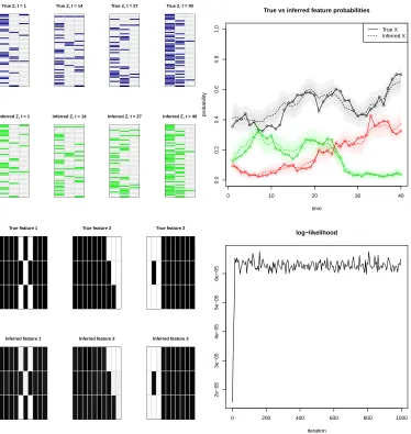
Figure 4-top-left compares the true underlying feature matrices at timest={1,14,27,40} in terms of the most frequently active features in the posterior mean matrices, where a fea-ture is set to be active if that is the case in more than half of the samples of the Markov chain. The resulting mean matrices almost perfectly match the true underlying feature matrices. Figure 4-top-right compares the trajectories over time of the true feature prob-abilities with the inferred ones. The latter tend to be less than two standard deviations away from the former, meaning that the true feature trajectories are closely tracked. Figure 4-bottom-left compares the three features represented by the true factor matrix A and the ones in the posterior mean matrix ˆA, showing that the algorithm was able to recover accu-rately the hidden features underlying the noisy observations. Figure 4-bottom-right plots the log-likelihood at each iteration, showing that the algorithm converged quickly, namely in fewer than 50 iterations.
Then, we tested the ability of the slice sampler-based algorithm to recover the correct number of latent features when given a similar set of synthetic data, this time consisting of 4 latent features evolving over 6 time points. The algorithm was initialized with one feature and run for 3300 iterations with a burn-in period of 1000 iterations. As in the finite case, the true underlying feature allocation matrices and feature probabilities were closely recovered as illustrated by the top row of Figure 5. The bottom row of Figure 5 shows that the features were reconstructed accurately and their correct number detected in about 700 iterations.
True Z, t = 1 True Z, t = 14 True Z, t = 27 True Z, t = 40
Inferred Z, t = 1 Inferred Z, t = 14 Inferred Z, t = 27 Inferred Z, t = 40
0 10 20 30 40
0.0 0.2 0.4 0.6 0.8 1.0
True vs inferred feature probabilities
time probability ● ●● ● ● ● ● ● ● ● ● ● ● ● ● ● ●● ●● ● ● ● ● ● ● ● ● ● ●●● ●● ● ● ● ● ● ● ● ● ● ● ● ● ● ● ●● ● ● ● ● ● ●● ● ● ● ● ●●● ● ● ● ●● ● ●● ● ●● ● ● ● ●● ●● ● ● ● ● ● ● ●● ● ● ● ● ● ● ● ● ● ● ● ● ● ● ● ● ● ● ● ● ●● ● ●● ● ● ●● ● True X Inferred X
True feature 1 True feature 2 True feature 3
Inferred feature 1 Inferred feature 2 Inferred feature 3
0 200 400 600 800 1000
[image:21.612.126.500.152.547.2]2e−05 3e−05 4e−05 5e−05 6e−05 log−likelihood iteration
True Z, t = 1 True Z, t = 2 True Z, t = 3 True Z, t = 4 True Z, t = 5 True Z, t = 6
Inferred Z, t = 1 Inferred Z, t = 2 Inferred Z, t = 3 Inferred Z, t = 4 Inferred Z, t = 5 Inferred Z, t = 6
1 2 3 4 5 6
0.0
0.2
0.4
0.6
0.8
1.0
True vs inferred feature probabilities
time
probability
True X Inferred X
True feature 1 True feature 2 True feature 3 True feature 4
Inferred feature 1 Inferred feature 2 Inferred feature 3 Inferred feature 4
0 500 1000 1500 2000 2500 3000
Inferred number of features
iteration
features
1
2
3
4
[image:22.612.122.530.158.570.2]5
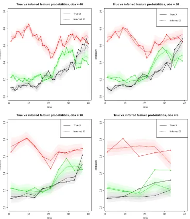
5 10 15 20 0.0 0.2 0.4 0.6 0.8 1.0
True vs inferred feature probabilities
time probability ● ● ● ● ● ● ● ● ● ● ● ● ● ● ● ● ● ● ● ● ● ● ● ● ● ● ● ● ● ● ● ● ● ● ● ● ● ● ● ● True X Inferred X ● ● ● ● ● ● ● ● ● ● ● ● ● ● ● ● ● ● ● ●
5 10 15 20
0.0 0.2 0.4 0.6 0.8 1.0
True vs inferred feature probabilities
[image:23.612.116.497.261.471.2]time probability ● ● ● ● ● ● ● ● ● ● ● ● ● ● ● ● ● ● ● ● ● ● ● ● ● ● ● ● ● ● ● ● ● ● ● ● ● ● ● ● ● ● ● ● ● ● ● ● ● ● ● ● ● ● ● ● ● ● ● ● True X Inferred X
0 10 20 30 40
0.0
0.2
0.4
0.6
0.8
1.0
True vs inferred feature probabilities, obs = 40
time
probability
True X
Inferred X
0 10 20 30 40
0.0
0.2
0.4
0.6
0.8
1.0
True vs inferred feature probabilities, obs = 20
time
probability
True X
Inferred X
0 10 20 30 40
0.0
0.2
0.4
0.6
0.8
1.0
True vs inferred feature probabilities, obs = 10
time
probability
True X
Inferred X
0 10 20 30 40
0.0
0.2
0.4
0.6
0.8
1.0
True vs inferred feature probabilities, obs = 5
time
probability
True X
[image:24.612.113.504.144.594.2]Inferred X
7. Topic modeling application
In this section we apply the WF-IBP to the modeling of corpora of time-stamped text documents. This is a natural application as documents can be seen as arising from an unknown number of latent topics whose popularity is evolving over time. A related model to achieve this goal is described in Blei and Lafferty (2006), where a Gaussian state space model captures the evolution of topics in such a way that both the content of topics and their proportions evolve over time. This work has had a great impact in the topic modeling community, and anticipates a number of directions for future work that we address here. Specifically their model is parametric, in that the number of topicsK is fixed and needs to be pre-specified. The authors claim that it would desirable to drop this assumption to have a more flexible model and, in particular, foresee a process involving births and deaths of topics. The WF-IBP topic model elegantly achieves these goals. Unlike Blei and Lafferty (2006) we focus on the evolution of topic probabilities rather than topic contents, noting that the modeling of time-varying topic contents is orthogonal to our work and could be incorporated into the WF-IBP in future developments. Another class of models called Dirichlet processes aim at modeling the evolution of topics in a time-dependent and nonparametric way. Some of these models, however, assume the evolution of topic probabilities to be unimodal (e.g., Rao and Teh, 2009), while others are HDP-based (Ahmed and Xing, 2012; Dubey et al., 2013) and implicitly assume a positive correlation between the probability of a topic being active and the proportion of that topic within each document. Coupling topic proportions and topic probabilities is undesirable as rare topics may account for a large proportion of words in the few documents in which they appear. Our nonparametric topic model decouples the probability of a topic and its proportion within documents and offers a flexible way to model topic evolutions over time. We achieve this by incorporating time-dependency into the focused topic model presented in Williamson et al. (2010b), which makes use of the IBP to select the finite number of topics that each document treats.
7.1 The WF-IBP topic model
First consider the case in which the number of topics K underlying the corpus of seen documents is known. Define topics as probability distributions over a dictionary of D
words and model them as (ρk)Kk=1
iid
∼ Dirichlet(¯η),given a vector ¯η of length D. Let ρ be the resulting vector and assume the components of ¯η to be all equal to a constant η >0. Consider the usual setting in which the time-dependent popularity of topic (feature) k is denoted byXk and the binary variablesZikt indicate whether document icontains topick
at timet. Then, for all t=t0, . . . , tT and k= 1, . . . , K, sample
θit | {Zit=zit, φt=φ0t} ∼Dirichlet(zit◦φ0t), ∀i= 1, . . . , Nt,
φkt∼Gamma(γ,1),
(Zikt)Ni=1t | {Xk=xk(t)}iid∼Bernoulli(xk(t)),
Xk ∼WF
αβ K, β
,
where φkt is the kth component of φt, a K-long vector of topic proportions, and θit the
time t. The operation zit◦φt stands for the Hadamard product between zit and φt and
the Dirichlet is defined over the positive components of the resulting vector. While the topic allocation matrix Zt encodes which subset of theK topics appears in each document
at time t, the variables φkt are related to the proportion of words that topic k explains
within each document. Unlike HDP-based models, these two quantities are here modeled independently.
For every document i = 1, . . . , Nt, draw the total number of words from a
negative-binomialWit∼NB(Pkziktφkt,1/2) and, for each wordwilt, l= 1, . . . , Wit, sample first the
topic assignment
ailt| {θit=θit0 } ∼Categorical(θ 0 it)
and then the word
wilt | {ailt=a0ilt, ρ=ρ
0} ∼
Categorical(ρ0a0
ilt).
Assume now that the number of potential topics K needs to be learned from the data. The nonparametric extension of this model is easily obtained by replacing the process generating the topic allocation matrices with the WF-IBP, so that topics arise as in the PRF and evolve as independent WF(0, β). The feature allocation matrices can be drawn as described in Section 8. In this way, we obtain a time-dependent extension of the IBP compound Dirichlet process presented in Williamson et al. (2010b).
7.2 Posterior inference
In order to infer the latent variables of the model, it is convenient to integrate out the parametersρ andθ. This can be done easily thanks to the conjugacy between the Dirichlet and the Categorical distribution. In this way, we can run a Gibbs sampler for posterior inference only over the remaining latent variables and are able to follow the derivation of conditionals given by Williamson et al. (2010a). Note that, in our case, we have introduced the slice variable and do not integrate out the topic allocation matrix. Denote by W the complete set of words and by A the complete set of topic assignments ailt for all times
t = t0, . . . , tT, documents i = 1, . . . , Nt and words l = 1, . . . , Wit. Denote by St the slice
variable and by Wt the complete set of words at timet. The conditional distributions that
we need to sample from for all timest=t0, . . . , tT are
p(At|Zt, w, φt),
p(φt, γ|At, Wt, Zt),
p(St|Zt, X(t)),
p(Zt|At, X(t), φt, St).
Conditioning on all the other topic assignments a−il, each topic assignment ailt can be
sampled from
p(ailt=k|a−il, Zt, W, φt)∝(nwkil+η)
nikt+φktzikt
nk+ηD−1
wherenwil
k denotes the number of times that word wil has been assigned to topick
exclud-ing assignment ail, nikt the number of words assigned to topic k in document i excluding
assignmentail and nk the total number of words assigned to topick.
After placing a hyper-prior on p(γ), we can sample φ and γ via a Metropolis-Hastings step. Indeed, we know that
p(φkt, γ|A, Zt)∝
φγkt−1e−φkt
Γ(γ) p(γ)
Nt
Y
i=1
Γ(φktzikt+nikt)
Γ(φktzikt)nikt!2φktzikt+n
i kt
.
Conditioning on Zt, the slice variable is sampled according to its definition:
p(St|Zt, X(t)) =
1
xmin(t)1st([0, x
min(t)]),
where xmin(t) is the minimum among the probabilities of the active topics at time t. As
for the feature allocation matrices Z, we sample only the finite number of its components whose topic probabilityxk(t) is greater than the slice variableSt. Assume we are sampling
each entry Zikt sequentially and denote respectively by xmin1 (t) and xmin0 (t) the minimum
active topic probability in the casesZikt= 1 andZikt= 0. Letnikt denote the total number
of words assigned to topick in documentiat time t. Then we have that
p(Zikt= 1|A, xk(t), φkt) =
1, ifnikt>0
xk(t)xmin
0 (t)
xk(t)xmin0 (t)+2φkt(1−xk(t))xmin1 (t)
, ifnikt= 0.
p(Zikt= 0|A, xk(t), φkt) =
0, ifnikt>0
2φkt(1−xk(t))xmin
1 (t)
xk(t)xmin
0 (t)+2φkt(1−xk(t))xmin1 (t)
, ifnikt= 0.
The full conditional distributions presented so far are derived in Appendix C. As in the linear-Gaussian case, when considering the probability of settingZikt = 1 for a feature that
is currently inactive across all observations at time t, it is necessary to jointly propose a new valueφkt by drawing it from its prior distribution Gamma(γ,1). Finally, inference on
the trajectories of the topic probabilities is a direct application of the Particle Gibbs and thinning scheme outlined for the general case.
7.3 Topic model: simulation and results
and the algorithm was able to infer closely the latent topic allocation matrices (Figure 9-left). The percentage of words assigned to the correct topics were 81% at t1, 82% at t2, 83% att3 and 85% att4.
A Monte Carlo estimate for the probability of word w= 1, . . . , D under topic kis
ˆ
ρkw=
nwk +η nk+Dη
,
wherenwk is the number of times wordwhas been assigned to topick,nkis the total number
of words assigned to topickandDis the number of words in the dictionary. A Monte Carlo estimate for the probability of topickin document iis
ˆ
θikt =
nikt+ziktφkt
P
k(nikt+ziktφkt)
. (11)
These two quantities are given by the posterior mean of the Dirichlet distribution under a categorical likelihood. ˆρkw has been used to plot the posterior distribution over words in
Figure 9-right. These results confirm the ability of the algorithm to recover ground truth and provide useful information both at word and topic level.
Finally, we tested the ability of the algorithm to reconstruct topics when presented with a decreasing number of observed documents. 100 documents were simulated at each of two time points as described above. Figure 10 shows how well the probability of the 10 most likely words of the first topic was reconstructed for N = 60, 40, 20 and 10 observed documents per time point. As expected, the more documents are observed the more accurate the reconstruction of topics is, with a drop in performance when only 10 documents per time point are observed.
0 500 1000 1500 2000 2500 3000
39
40
41
42
train negative log-likelihood
[image:28.612.155.462.449.667.2]iterations
True Z, t = 1 True Z, t = 2 True Z, t = 3 True Z, t = 4
Inferred Z, t = 1 Inferred Z, t = 2 Inferred Z, t = 3 Inferred Z, t = 4
[image:29.612.119.501.266.453.2]True word probabilities Inferred word probabilities
0.0
0.2
0.4
N = 60
1 2 3 4 5 6 7 8 9 10
true inferred
0.0
0.2
0.4
N = 40
1 2 3 4 5 6 7 8 9 10
true inferred
0.0
0.2
0.4
N = 20
1 2 3 4 5 6 7 8 9 10
true inferred
0.0
0.2
0.4
N = 10
1 2 3 4 5 6 7 8 9 10
[image:30.612.112.503.234.489.2]true inferred
7.3.1 Comparison: static model and hierarchical model
We now demonstrate the advantages of modeling time-dependency by comparing our model with two alternative versions. First, we consider a static counterpart where time is not mod-eled and thus information about the time-stamp of documents is not exploited. Second, we consider a hierarchical model where feature probabilities at each time point are distributed as conditionally independent beta processes given a lower-layer beta process (Thibaux and Jordan, 2007); note that in this model observations at different time points are modeled separately, but information on the order of the time points is ignored.
In particular, we investigate whether incorporating time into the model improves upon test-set perplexity, a measure widely used in topic modeling settings that assesses the ability of topic models to generalize to unseen data. Given the model parameters Φ, perplexity on documents Dtest :={di}Mi=1 is defined as
perplexity(Dtest|Φ) = exp −
PM
i=1log p(di|Φ)
PM
i=1Wi
!
,
where Wi denotes the number of words in document di. As we assume that words within
each document are drawn independently given the model parameters Φ, the probability of documentdi can be computed as
p(di|Φ) = Wi
Y
l=1
p(wil |Φ),
where
p(wil|Φ) = K
X
k=1 θikρkl,
recalling thatθikis the probability of a generic word belonging to topickin documentiand
ρkl is the probability of word l under topick. These two quantities can be approximated
at each iteration of the MCMC algorithm by their current values ˆθ(iks) and ˆρ(kls), so that we can approximate the probability of each word by averaging over S samples of the Markov Chain.
ˆ
p(wil|Φ) =
1
S
S
X
s=1
K
X
k=1
ˆ
θik(s)ρˆ(kls).
Note that the perplexity is inversely proportional to the likelihood of the data and thus lower values indicate better performance. Chance performance, namely assuming each word to be picked uniformly at random from the dictionary, yields a perplexity equal to the sizeD
of the dictionary.
to generate 30 documents at each of 9 time points. The number of features was fixed to 4 and the algorithms were run 3000 iterations with a burn-in period of 300 iterations. Even though all three algorithms approximately recover the true topic allocations matrices, incorporating time leads to a closer match. This can be measured, for instance, by the Frobenius norm of the difference between each true and inferredZt. Table 1 shows that at
[image:32.612.92.533.404.646.2]each time the dynamic model leads to a lower discrepancy with the true topic allocation matrix. Figure 11 shows the posterior trajectories of topic probabilities inferred by the dynamic model and compares them with the posterior feature probabilities inferred by the hierarchical model and the constant values inferred by the static model. It can be observed that the trajectories inferred by the dynamic model are both smoother and closer to the ground truth. Finally, Figure 12 compares the test-set perplexity of the three models (recall that in this case chance performance results in a perplexity of D = 1000). As expected, although the hierarchical version performs better than the static counterpart that neglects time-stamp information, it is outperformed by our dynamic model. Indeed, while in the WF-IBP observations that are closer in time exhibit a stronger dependency, the HBP does not explicitly impose an ordering of the time points. The results show that having a suitable model for time dependencies improves on the ability to recover ground truth as well as to generalize to unseen data.
Table 1: Frobenius norm of the difference with the trueZt. The lower, the better.
t1 t2 t3 t4 t5 t6 t7 t8 t9 Dynamic 1.78 1.37 0.72 2.99 3.24 2.01 2.59 2.45 2.88 Hierarchical 1.94 1.51 2.80 3.11 3.52 2.91 2.65 2.59 3.24
Static 3.63 4.23 2.84 3.01 3.55 5.27 4.89 3.31 5.90
2 4 6 8
0.0
0.2
0.4
0.6
0.8
1.0
Dynamic model
time
p
ro
b
a
b
ili
ty
2 4 6 8
0.0
0.2
0.4
0.6
0.8
1.0
Hierarchical model
time
2 4 6 8
0.0
0.2
0.4
0.6
0.8
1.0
Static model
time
220
260
300
340
pe
rp
le
xi
ty
5% held-out data
true dyn hbp stat
220
260
300
340
pe
rp
le
xi
ty
10% held-out data
true dyn hbp stat
220
260
300
340
pe
rp
le
xi
ty
20% held-out data
true dyn hbp stat
220
260
300
340
pe
rp
le
xi
ty
30% held-out data
true dyn hbp stat
220
260
300
340
pe
rp
le
xi
ty
40% held-out data
true dyn hbp stat
220
260
300
340
pe
rp
le
xi
ty
50% held-out data
[image:33.612.126.491.118.345.2]true dyn hbp stat
Figure 12: Boxplots of test-set perplexity for different percentages of held-out data for the true model (true), our dynamic model (dyn), the hierarchical version (hbp) and the static version (stat). Each boxplot was obtained by computing the perplexity after holding-out 10 different random subsets of words in the data. Lower values indicate better performance.
7.3.2 Real-world data experiments
We used the WF-IBP topic model to explore the data set consisting of the full text of 5811 NIPS conference papers published between 1987 to 2015.1 We pre-processed the data and
removed words appearing more than 5000 times or fewer than 250 times. The remaining number of word tokens was 4 728 892 with a vocabulary size of 348 672 unique words. Our goal was to discover what topics appear in the corpus and to track the evolution of their popularity over these 29 years.
We set the hyperparameters α and β equal to 1 and the time step to 0.12 diffusion time-units per year so as to reflect realistic evolutions of topic popularity. The Markov chain was run for 2000 iterations with a burn-in period of 200 iterations, settingη= 0.001 and placing a Gamma(5,1) hyper-prior onγ.
Qualitative results One of the qualitative advantages of modeling time dependency explicitly is that interesting insights into the evolution of topics underlying large collections of documents can be obtained automatically, and uncertainty in the predictions naturally incorporated. The 12 most likely words of 32 topics found in the corpus together with the evolution of their topic proportions are given in Figure 13, where the shaded areas
1. The data set is available at https://archive.ics.uci.edu/ml/datasets/NIPS+Conference+Papers+