Latent Constrained Correlation Filter

(1)

Latent Constrained Correlation Filter

Baochang Zhang, Shangzhen Luan, Chen Chen, Jungong Han, Wei Wang, Alessandro Perina,

and Ling Shao, Senior Member IEEE

Abstract—Correlation filters are special classifiers designed for shift-invariant object recognition, which are robust to pattern distortions. The recent literature shows that combining a set of sub-filters trained based on a single or a small group of images obtains the best performance. The idea is equivalent to estimating variable distribution based on the data sampling (bagging), which can be interpreted as finding solutions (variable distribution approximation) directly from sampled data space. However, this methodology fails to account for the variations existed in the data. In this paper, we introduce an intermediate step – solution sampling – after the data sampling step to form a subspace, in which an optimal solution can be estimated. More specifically, we propose a new method, named latent constrained correlation filters (LCCF), by mapping the correlation filters to a given latent subspace, and develop a new learning framework in the latent subspace that embeds distribution-related constraints into the original problem. To solve the optimization problem, we introduce a subspace based alternating direction method of multipliers (SADMM), which is proven to converge at the saddle point. Our approach is successfully applied to three different tasks, including eye localization, car detection and object tracking. Extensive experiments demonstrate that LCCF

outperforms the state-of-the-art methods.1

Index Terms—Correlation filter, ADMM, Subspace, Object detection, Tracking

I. INTRODUCTION

Correlation filters have attracted increasing attention due to its simplicity and high efficiency. They are usually trained in the frequency domain with the aim of producing a strong correlation peak on the pattern of interest while suppressing the response to the background. To this end, a regression process is usually used to obtain a Gaussian output that is robust to shifting. Recently, correlation filters have emerged as a useful tool for a variety of tasks such as object detection and object tracking.

The correlation filter method is first proposed by Hester and Casasent, named synthetic discriminant functions (SDF)

The work was supported in part by the Natural Science Foundation of China under Contract 61672079 and 61473086. This work is supported by the Open Projects Program of National Laboratory of Pattern Recognition. (B. Zhang and S. Luan contributed equally to this work.) (Corresponding author: Jungong Han.)

B. Zhang, S. Luan and W. Wang are with the School of Automation Science and Electrical Engineering, Beihang University, Beijing, China. Email: bczhang@buaa.edu.cn.

C. Chen is with Center for Research in Computer Vision (CRCV), University of Central Florida, Orlando, FL, USA. Email: chenchen870713@gmail.com.

J. Han is with the School of Computing and Communications, Lancaster University, Lancaster LA1 4YW, U.K. Email: jungonghan77@gmail.com.

A. Perina is with Microsoft Corporation, Redmond, WA, USA.

L. Shao is with the School of Computing Sciences, University of East Anglia, Norwich NR4 7TJ, U.K. Email: ling.shao@ieee.org.

Manuscript received XX XX, 2016.

1_The _source _code _will _be _publicly _available.

https://github.com/bczhangbczhang/

[13], which focuses more on formulating the theory. Later on, to facilitate more practical applications, many variations are proposed to solve object detection and tracking problems. For object detection task, early research can be traced back to [23], where Abhijitet al.synthesize filters by Minimizing the Average Correlation plane Energy (MACE), thus allowing easy detection in the full correlation plane as well as control of the correlation peak value. In their improved work [25], it was noted that the hard constraints of MACE cause issues with distrotion tolerance. Therefore, they eliminate the hard constraints and require the filter to produce a high average correlation response instead. A newer type of CF, named Average of Synthetic Exact Filters (ASEF) [3], tunes filters for particular tasks, where ASEF specifies the entire correlation output for each training image, rather than specifying a single peak vaule used in earlier methods. Despite its better capability of dealing with the over-fitting problem, the need of a large number of training images makes it difficult for real-time applications. Alternatively, Multi-Channel Correlation Filters (MCCF) [15] take advantage of multi-channel features, such as Histogram of Oriented Gradients (HOG) [34] and Scale-Invariant Feature Transform (SIFT) [20], in which each feature responds differently and the outputs are combined to achieve high performance. For the tracking task, Minimum Output Sum of Squared Error filters (MOSSE) [2] are considered as the earliest CF tracker, which intends to produce ASEF-like filters from fewer training images. Its essential part is a mapping from the training inputs to the desired training outputs by minimizing the sum of squared error between the actual output of the convolution and the desired output of the convolution. Alternatively, Kernelized Correlation Filters (KCF) [12] map the feature to a kernel space, and utilize the properties of the cyclic matrix to optimize the solution process. Since then, most trackers are improved based on KCF, such as [19], [40], [27], [22], [33]. We provide a comprehensive review of these approaches in the next section.

(2)

an adaptive multi-class correlation filters (AMCF) method is introduced based on an alternating direction method of multipliers (ADMM) framework by considering the multiple-class output information in the optimization objective.

Problem: Given the training samples, at the core of

cor-relation filtering is to find the optimal filters, which requires the unknown variable distribution estimation. Traditional al-gorithms normally adopt one of the following schemes: 1) finding a single filter (i.e., channel filter [15]) trained by a regression process based on all training samples [15], [16], and 2) finding a set of sub-filters (a single filter per image [3]) and eventually integrating them into one filter. Here, the combination can be either based on averaging the sub-filters in an off-line manner [3] or an on-line iterative updating procedure [12], which is similar to that of the bagging method [17]. Revealed by the literature, the performance of the second scheme is better than that of the first one [12], even though it is computationally more expensive. The second scheme is equivalent to estimating solution distribution based on only a limited amount of sampled data, which fails to consider the variations existed in the data in the optimization objective.

One fact that has been overlooked in correlation filter learning is that data sampling (bagging) can actually lead to solution sampling, which is traditionally used to find an ensemble classifier. However, we argue that the bagging results can also be used to estimate the distribution of the solutions. Then, the distribution (later subspace) in turn can be deployed to constrain and improve the original solution. In this paper, we attempt to implement the above idea in correlation filtering, in order to enhance the robustness of the algorithm.

The framework of the proposed Latent Constrained Corre-lation Filters (LCCF) is shown in Fig. 1. To find the solution sampling in the training process, unlike an ad-hoc way that directly inputs all samples to train correlation filters, we train sub-filters step by step based on iteratively selecting subsets. Instead of estimating a real distribution for an unsolved variable that is generally very difficult, we exploit sampling solutions to form a subspace, in which the bad solution from a noisy sample set can theoretically be recovered after being pro-jected onto this subspace in an Alternating Direction Method of Multipliers (ADMM) scheme. Eventually, we can find a better result from the subspace (subset) that contains different kinds of solutions to our problem. From the optimization perspective, the subspace is actually used to constrain the solution, as shown in Fig. 1. In fact, the above constrained learning method is a balanced learning model across different training sets. The application of constraints derived from data structure in the learning model is capable of achieving good solutions [6], [5], [36]. This is also confirmed by [5], in which the topological constraints are learned by using data structure information. In [36], Zhang et al.put forward a new ADMM method, which can include manifold constraints during the optimization process of sparse representation classification (SRC). These methods all achieve promising results by adding constraints.

Another key issue is how to efficiently embed the subspace constraints in the optimization process. In this paper, we propose a Subspace based Alternating Direction Method of

Multipliers (SADMM). The classical ADMM is an algorithm that solves convex optimization problems by breaking them into smaller pieces, and each of which can be handled easily [4]. However, the original ADMM cannot be directly applied to solve our problem due to its infeasibility of handling the subspace constraint. In contrast, the proposed SADMM is more flexible and proved to converge at the saddle point, therefore enabling a faster algorithm. In summary, our LCCF based on SADMM differ from the previous approaches in two aspects:

1) Our SADMM takes advantage of the inherent visual data structure for solving the optimization problem. We show that SADMM theoretically converges at the saddle point in an efficient way.

2) Our SADMM can be used to solve both linear and kerner-lized correlation filtering based on a latent subspace constraint. Experimental results show that it consistently outperforms the state-of-the-art methods on three different tasks, i.e., eye localization, car detection and object tracking, revealing the generalization ability of the proposed SADMM model.

Notation: In this paper, T is the transpose operator of

matrix. The operatordiag converts the D dimensional vector into aD×D dimensional matrix, which is diagonal with the original vector. The subscript i represents the ith element in a data set (i.e., xi refers to the ith sample in a training set or a test set), the subscript [k] represents channel (i.e., xi,[k]

represents thekth_{channel of}_x_i,_h

[k]refers to thekthchannel

of h), and the superscript refers to the iterations of variable (i.e.,hˆt_{for the variable}_hˆ _{in the}_tth_{iteration). For clarity, we} summarize main variables in Table I.

II. RELATED WORK

Comparing with the traditional object detection and tracking algorithms [34], [14], [10], [35], [39], correlation filtering exploits convolution to simplify the mapping between the input training image and the output correlation plane, and has high computational efficiency and strong robustness. A flurry of recent extensions to correlation filter have been successfully used in the object detection and tracking applications.

Bolme et al. propose a method to learn several accurate weak classifiers to construct a strong classifier for eye local-ization [6]. Later, they propose to learn a Minimum Output Sum of Squared Error (MOSSE) filter [5] for visual tracking on gray-scale images, which is very efficient with a speed reaching several hundreds frames per second. Heriqueset al.

(3)

Frame t+1 Frame t

Frame 2 Frame 1

Frame 0

Training Set Training Set Training Set

...

A Latent Constrained Subspace

A detection training process

A tracking task training process



SADMM

...

0

 1 2 t t1

0

h _h1 _ht1

or

1 t+1



t

h



1t_or 1t

g



[image:3.612.60.545.262.356.2]

Updatinghor 

Fig. 1. The framework of the proposed latent constrained correlation filters (LCCF). In the left-upper part, we show a detection training process.hˆ0:t+1

forms a subspace, in whichgˆt+1_{is obtained based on a projection}_Φ_{. In the left-bottom part, we show a tracking process.}_α_ˆ0:t+1_{forms a subspace, in which}

ˆ

βt+1_{is obtained based on a projection}_Φ_{. This procedure leads to a Subspace based Alternating Direction Method Of Multipliers (SADMM) algorithm.}

TABLE I

ABRIEF DESCRIPTION OF VARIABLES AND OPERATORS USED IN THE PAPER.

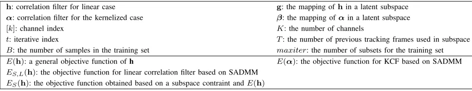
h: correlation filter for linear case g: the mapping ofhin a latent subspace

α: correlation filter for the kernelized case β: the mapping ofαin a latent subspace

[k]: channel index K: the number of channels

t: iterative index T: the number of previous tracking frames used in subspace

B: the number of samples in the training set maxiter: the number of subsets for the training set E(h): a general objective function ofh E(α): the objective function for KCF based on SADMM ES,L(h): the objective function for linear correlation filter based on SADMM

ES(h): the objective function obtained based on a subspace contraint andE(h)

of a target object and learn an adaptive correlation filter by mapping multi-channel features into a Gaussian kernel space [8]. In [7], Discriminative Scale Space Tracker (DSST) is proposed to handle scale variations based on a scale pyramid representation. This scale assessment method can also be embedded into other models [27], [22]. Ma et al. develop a re-detecting process to further improve the performance of KCF [22]. In [16], Galoogahi et.al present a method to limit the circular boundary effects while preserving many of the computational advantages of canonical frequency domain correlation filters. In [21], convolutional features correlation filters (CFCF) exploit features extracted from deep convolu-tional neural networks (DCNN) trained on object recognition datasets to improve tracking accuracy and robustness.

From the review of previous works, it can be seen that the distribution introduced by the bagging method is not well studied for the correlation filter calculation. However, the distribution information is important to calculate robust filters, especially when the data suffer from severe noise, occlusion, etc.

III. SUBSPACE BASED ALTERNATING DIRECTION METHOD OF MULTIPLIERS(SADMM)

The Augmented Lagrangian Multiplier (ALM) methods are a class of algorithms for solving constrained optimization problems by including penalty terms to the objective function [28]. As a variant of the standard ALM method that uses partial updates (similar to the Gauss-Seidel method for solving linear equations), ADMM recently gained much more attention due to its adaptability to several problems [4]. By solving iteratively a set of simpler convex optimization sub-problems,

each of which can be handled easily. In this section, we show how the visual data structure, i.e., subspace constraints, can be embedded into the ALM minimization to define SADMM. We then present the resulting algorithm for the proposed SADMM and the solution of each sub-problem.

The primary task is to minimizeE(ˆh)that is a general and convex optimization objective. In order to exploit the property of solution sampling from the data sampling, the subspace constraint is added to the original optimization problem. That is to say, instead of estimating a real distribution function of any unsolved variable, the problem can be solved based on a subspace containing the sub-solutions. Specifically, we add a new variable in the optimization problem, which is

ˆ

g representing the mapping of hˆ in a specific subspace:

ˆ

h → gˆ ∈ S. The goal is to explicitly impose the subspace constraints by the cloned variables, though this will inevitably bring extra storage costs due to the replicated variables. We have a new optimization problem as:

minimize E(ˆh)

subject to hˆ = ˆg; ˆg∈ S, (1)

whereS refers to a well-designed subspace. ALMs are used to solve the problem via

ES(ˆh) =E(ˆh) +RT(ˆg−hˆ) +σ₂||ˆg−h||ˆ 2, (2)

(4)

ˆ

ht+1= argminES(ˆh|gˆt) (3)

ˆ

gt+1_{= argmin}_E

S(ˆg|hˆt+1)

subject to gˆ∈ S. (4)

Different from Eq. (3) that can be easily solved using an ex-isting optimization method, i.e., Gradient descent, the solution of Eq. (4) becomes complex due to the new constraint of g∈ S. We rewrite Eq. (4) by dropping the index for an easy presentation:

ˆ

g= argminRT_(ˆ_g₋_hˆ_{) +}σ

2||ˆg−h||ˆ 2_,

subject to gˆ∈ S. (5)

By dropping constant terms, Eq.(5) is equivalent to:

ˆ

g= argmin||ˆg−(ˆh−R

σ)||

2_,

subject to ˆg∈ S. (6)

The solution to Eq.(6) is given by: ˆg = Ms(ˆh− _σr), where Ms is the projection matrix related to the subspace of the solutions to our problem. R is omitted to obtain the ADMM scheme from the original ALM method [36]. This also improves the efficiency of our method. Thus, we have:

ES(ˆh) =E(ˆh) +σ₂||gˆ−h||ˆ 2. (7)

In the relaxed versiongˆ is only considered to be recovered by S (Ms) built fromh, which is defined by the functionˆ Φ

discussed later. This leads to a new ADMM method, named subspace based ADMM (SADMM) algorithm, which makes use of an iterative process similar to that in [4]. Specifically, after the variable replication, ˆg is calculated according to a given subspace. This means that we could findhˆt+1based on

ˆ

ht and gˆt in the tth iteration. Next, we expand the training set by adding a number of training samples.gˆt+1is calculated based on the subspace spanned by hˆ0:t+1 ((Ms)), which includes sub-filters fromhˆ0(initialized) tohˆt+1. This iterative process is described as follows:

ˆ

ht+1_{= argmin}_E

S(ˆh|gˆt),

ˆ

gt+1= Φ(ˆht+1,hˆ0:t). (8)

It should be noted that the theoretical investigation into our SADMM algoritm shows that the convergence speed of SADMM is as fast as ADMM [4], which is elaborated in the appendix part.

IV. LATENT CONSTRAINED CORRELATION FILTERS

A. Correlation filters

The solution to correlation filters, i.e., multiple-channel correlation filter, can be regarded as an optimization problem which minimizes E(h). This procedure can be described by the following objective function:

E(h) = 1 2

N

X

i=1

||yi− K

X

k=1

h_[_k_]T ⊗xi,[k]||22+

1 2

K

X

k=1

||h_[_k_]||2 2,

(9)

where N represents the number of images in the training set, and K is the total number of channels. In Eq. (9), xi refers to a K-channel feature/image input which is obtained in a texture feature extraction process, while yi is the given response whose peak is located at the target of interest. k

represents the kth_{-channel. The single-channel response is a}

D dimensional vector, yi = [y(1), ...,y(D)]T _∈

RD. Both

xi andh are K×D dimensional super-vectors that refer to multi-channel image and filter, respectively. Correlation filters are usually constructed in the frequency domain. Therefore, to solve Eq. (9) efficiently, we transform the original problem into the frequency domain by the Fast Fourier Transform (FFT), which becomes:

E(ˆh) = 1 2

N

X

i=1

||ˆyi− K

X

k=1

diag(ˆxi,[k])

T_ˆ h_[_k_]||2

2+

λ

2

K

X

k=1

||ˆh_[_k_]||2 2,

(10) whereh,ˆ x, andˆ yˆ refer to the Fourier form ofh, x, and y, respectively. Eq. (10) can be further simplified to:

EL(hˆ) =

1 2

N

X

i=1

||ˆyi−Xˆiˆh||22+

λ

2||

ˆ h||2

2, (11)

where

ˆ

h= [hˆT_[1], ...,ˆhT_[_k_]]T

ˆ

Xi = [diag(ˆxi,[1]), ...,diag(ˆxi,[k])]

(12)

A solution in the frequency domain is given by:

ˆ

h= (λI+

N

X

i=1

ˆ XTiXiˆ )−

1

N

X

i=1

ˆ

XTiyiˆ. (13)

Here, since Xi is usually a sparse banded matrix, one can actually transform solving the KD×KD linear system into solvingDindependentK×Kdimensional linear systems. By doing so, the correlation filters calculation exhibits excellent computational and memory efficiency.

B. Latent constrained linear correlation filter (LC-LCF) based on SADMM

In order to solve Eq. (11) based on SADMM, we reformu-late it using the subspace constraint as:

minimize EL(ˆh)

subject to hˆ = ˆg; ˆg∈ S. (14)

The objective function in Eq. (14) can be expressed as:

ES,L(ˆh) = 1₂ B

P

i=1

||yiˆ −Xiˆ h||ˆ 2

2+λ2||h||ˆ 2

2+σ2||gˆ−h||ˆ 2_,

(15) where λ and σ are regularization terms. According to SADMM, the solution is described as follows:

ˆ

ht+1_{= argmin}_E

L,S(ˆh|ˆgt),

ˆ

(5)

Algorithm 1 LC-LCF based on SADMM

1: Setk= 0,εbest= +∞,η= 0.7

2: Initializeσ0= 0.25(suggested in [36])

3: Initializegˆ0 andhˆ0 based on MCCF

4: InitializeB,Bdenotes the size of half of training samples,

maxiter= 12

5: repeat

6: H=

B

P

i=1

( ˆXT

i Xˆi) +λI+σtI

7: hˆt+1₌_H−1

B

P

i=1

ˆ

XT

iYiˆ +σˆgt

8: ε=khˆt+1₋_hˆt_k

2

9: if ε < η×εbest then

10: σt+1=σt

11: εbest=ε

12: else

13: σt+1= 2σt

14: end if

15: gˆt+1= Φ(ˆht+1,hˆ0:t)

16: t←t+ 1,B←B+B/maxiter

17: until some stopping criterion, i.e., maximum number of

iteration (maxiter=12).

HereMsis defined to behˆ0:t. To solve Eq.(16), we calculate the partial derivatives of Eq. (15), and thus have:

∂ES,L(ˆht+1)

∂(ˆht+1₎ =

B

X

i=1

( ˆXT_iXˆi+λI+σI)ˆht+1

−XXˆTi Yiˆ −σˆg t

,

(17)

whereB is the size of the training set. We come to the result of hˆt+1_{, and have:}

ˆ

ht+1=H−1(

B

X

i=1

ˆ

XT_iYˆi+σtgˆt), (18)

where

H=

B

X

i=1

( ˆXT_iXˆi) +λI+σtI, (19)

thengˆt+1 is calculated as :

ˆ

gt+1= Φ(ˆht+1,hˆ0:t) =

t

X

i=0

ωihˆi, (20)

where ωi = _d1

i, and di is the Euclidean distance between

ˆ

ht+1 _and _hˆi_. _ω _{will be normalized by the} _L_{1 norm.After} several iterations, hˆt+1 _{converges to a saddle point, which}

is proved in Appendix I. The pseudocode of our proposed method is summarized in Algorithm 1. The LC-LCF is first initialized based on a half of the training samples, and then we add _maxiterB samples into the training set, which is one kind of data sampling. Subsequently, a set of sub-filters (solution sampling) are calculated, and further used to constrain our final solution.

Algorithm 2 - LC-KCF algorithm for object tracking

1: Initial target bounding box b1= [px, py, w, h],

2: Initialαˆ0 using KCF method,βˆ0= ˆα0,σˆ0= 0.0001 3: Initialbest=∞,c= 2,λ= 0.0001,t= 1,

4: InitialT

5: repeat

6: Crop out the search windows according to bt, and extract the HOG features for training

7: Compute the kernel matrixKxx

8: Updateη using Eq. (28)

9: Updateαˆt+1 using Eq. (29)

10: ift <=T then

11: Update βˆt+1 =Pt

i=0ωiαˆi

12: else

13: Update βˆt+1 ₌Pt

i=t−T+1ωiαˆi

14: end if

15: =||αˆt+1−αˆt|| 16: if < best then

17: σt+1₌_σt_, best=

18: else

19: σt+1₌_cσt

20: end if

21: Crop out the search window and extract the HOG features for testing

22: Compute the kernel matrix of the test frameKzx

23: Compute the correlation response as:yˆ=F−1₍_Kzx

ˆ

αt+1)

24: Select the coordinate of the maximal correlation re-sponse as the next location of tracking object

25: Updatebt+1

26: t←t+ 1

27: until End of the video sequence.

28: end

C. Latent constrained kernelized correlation filter (LC-KCF) based on SADMM

In kernelized correlation filter (KCF), similar to the linear case, filters learned on the previous frames can also be used to constrain the solution. Details about KCF can refer to Appendix II. If one frame is disturbed by occlusion and noise, the performance of the filter tends to drop. Our idea is that, with a subspace constraint, the filter is regularized by a projection into a well-defined subspace to achieve a higher performance. In other words, the samples of the previous frames are involved in the reconstruction process of the filter with different weights, therefore enhancing the robustness of the filters.

As described in the second KKT condition detailed in Appendix II, we can solve h in a dual space by setting

α = ₂θ_λ. For KCF, the latent constraint is actually made for

α. We introduce the constraint term β as the mapping ofα

(6)

rewritten as:

Lp=

M×N

X

i=1

ξ_it+12+

M×N

X

i=1

θ_it+1(yi−(ht+1)Tφi−ξit+1)

+λ(||ht+1_||2₋_C2₎₋_δt_||_αt+1₋_βt_||2

2.

(21) The superscript t refers to the frame index, and also denotes the iteration number. The solution to Eq. (21) based on the SADMM method also depends on the iterative process. The variables need to be updated include α, β, and punishment coefficient δ. The mapping function φi = φ(xi), which is used to calculate the kernel matrix K. Based on KCF, we come up with a new maximizing objective function E(α):

E(α) =−λ2

M×N

X

i=1

αt_i+12

+ 2λ

M×N

X

i=1

αt_i+1yi

−λ

M×N

X

i,j=1

αt_i+1αt_j+1Ki,j−δt M×N

X

i

(αt_i+1−β_it)2

−λC2.

(22) We can further simplify it as:

E(α) =−λ2(αt+1)T(αt+1) + 2λ(αt+1)Ty

−λ(αt+1)TKαt+1

−δt(αt+1−βt)T(αt+1−βt)−λB2.

(23)

By setting a variable substitution δt = λσt and taking derivatives w.r.t.(αt+1):

∂(E(α))

∂(αt+1₎ =−2λ

2_αt+1_{+ 2}_λ_y₋₂_λ_K_αt+1

−2λσt(αt+1−βt),

(24)

we come to the solution of αt+1 as:

αt+1= (K+λI+σtI)−1(y+σtβt). (25)

The kernel matrix K is a cyclic matrix, we transform Eq. (25) by Fast Fourier Transform (FFT) to avoid the inverse operation of matrices [12]:

K=FHKxxF, (26)

whereF is a discrete Fourier transform matrix, andFH_{is the} conjugate transpose operation.Kxxis the first row ofK, then we obtain

ˆ

αt+1= (Kxx+λ+σt)−1(ˆy+σtβˆt). (27)

By setting

η= (Kxx+λI+σtI)−1(Kxx+λI), (28)

we change Eq. (27) to another form

ˆ

αt+1=ηαˆ + (1−η) ˆβt. (29)

This means that for thetthframe, we can calculateαˆt+1based on βˆt_{, and then update} _β_ˆt+1 _{based on the subspace spanned}

0 0.05 0.1 0.15 0.2

0 0.5 1

Threshold

Lo

ca

liz

at

io

n6

ra

te

Results6of6different6parameter6maxiter

maxiter=9 maxiter=10 maxiter=11 maxiter=12 maxiter=13 maxiter=14 maxiter=15

0 1 2 3 4 5 6 7 8 9 10 11 12

0.4 0.6 0.8 1

Iterations

Lo

ca

liz

at

io

n6

ra

te

Results6of6different6iterations6when6maxiter=12

Threshold=0.1

Threshold=0.15

Threshold=0.2

Fig. 2. Left: the localization rates under different maximum iterations for LCCF. Right: the convergence of our method when fixing themaxiterto 12.

by αˆ0:t+1 as the linear case. The process mentioned above can be summarized as:

    

   

ˆ

αt+1=ηαˆ+ (1−η) ˆβt

ˆ

βt+1= Φ( ˆαt+1,αˆ0:t) =X

i

ωiαˆi

ˆ

σt+1=cσˆt

(30)

Similar to Eq. (20), ωi is calculated based on the Euclidean distance, and details about normalization refer to the source code.

V. EXPERIMENTS

0 0.05 0.1 0.15 0.2 0

0.5 1

Threshold

Lo

ca

liz

at

io

n

R

at

e

Gaussian noise 0.01

LC-LCF MCCF

0 0.05 0.1 0.15 0.2 0

0.5 1

Threshold

Lo

ca

liz

at

io

n

ra

te

Gaussian noise:0.05

LC-LCF MCCF

0 0.05 0.1 0.15 0.2 0

0.5 1

Threshold

Lo

ca

liz

at

io

n

ra

te

Gaussian noise:0.1

LC-LCF MCCF

0 0.05 0.1 0.15 0.2 0

0.5 1

Threshold

Lo

ca

liz

at

io

n

ra

te

Gaussian noise:0.3

[image:6.612.314.561.55.173.2]

LC-LCF MCCF

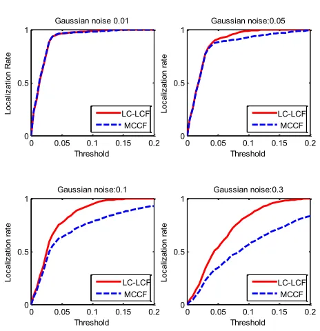
Fig. 3. The comparison between LCCF and MCCF on CMU Multi-PIE with different Gaussian noise parameters

[image:6.612.321.553.391.631.2]

(7)

located at the coordinate of target. All images are normalized before training and testing. The images are power normalized to have a zero-mean and a standard deviation of 1.0.

Subset, subspace and robustness evaluation for object

detection.We first introduce how to create different kinds of

subsets for calculating the sub-filers subspace. We add some noise or occlusions to the training and test sets in order to show how LC-LCF can gain robustness by a projection onto a subspace. More specifically, we first select an initial subset containing half of the training samples (the size was denoted byB). Other subsets are built by adding _maxiterB samples into the initial subset, where maxiter represents the maximum number of iterations. Based on the initial subset, we obtain

ˆ

h[0]_{, and calculate other sub-filters, i.e.,}_hˆt_{for the}_tth_iteration, step by step. With respect to the robustness evaluation, the basic idea for both applications is to measure the algorithm accuracy when adding Gaussian noise or occlusions to the training and test sets. For both applications, HOG feature is extracted by setting the number of direction gradients to 5, and both the sizes of block and cell to [5,5], as suggested in [15].

A. Eye localization

In the first experiment, the proposed method is evaluated for eye localization and compared with several state-of-the-art correlation filters, including MCCF [15], correlation filters with limited boundary (CFwLB) [16], ASEF [3] and MOSSE [2].

1) CMU Multi-PIE face database: The CMU Multi-PIE face database is used in this experiment. It consists of 902 frontal faces with neutral expression and normal illumination. We randomly select 500 images for training and the remaining for testing. All images are cropped to have a same size of 128 × 128 with fixed coordinates of the left and right eyes. We train a 128×128 filter of the right eye using full face images by following [15]. Similar to ASEF and MOSSE, we define the desired response as a 2D Gaussian function with a spatial variance of 2. Eye localization is performed by correlating the filters over the test images followed by selecting the peak of the output as the predicted eye location.

Results and analysis.In order to evaluate the performance

of our algorithm, we use the so-called fraction of interocular distance, which is defined by the actual and the predicted positions of the eyes. This distance can be computed as

d= ||pi−mi||2

||ml−mr||2

, (31)

where pi is the predicted location by our method, and mi is the ground truth of the target of interest, i.e., the eye’s coordinates ml andmr.

Haven calculated the distanced, the next step is to compare it with a threshold τ. If d < τ, the result will be considered as a correct one. We count the correct number under this threshold, and compute the ratio of the correct count to the total number of tests as the localization rate. The localization rates under differentmaxiters are shown in Fig. 2. We can see that LC-LCF obtains the best accuracy when maxiter= 12.

Ground Truth ASEF MOSSE MCCF CFwLB LC-LCF

0 0.05 0.1 0.15 0.2 0 0.5 1 Threshold Lo ca liz at io n ra te

No noise and no occlusion

ASEF MOSSE MCCF CFwLB LC-LCF

Slight occlusion test results

Slight noise test results

Occlusion and heavy noise

Fig. 4. The results of LC-LCF compared to the state-of-the-art correlation filters on CMU Multi-PIE. The variance is varying from 0.05 (slight) to 0.1 (heavy). On the left part, from the first column to the fourth column, we show results on the original images, images with occlusions, images with slight noise, and images with heavy noise and occlusions.

Some visualization results of LC-LCF

0 0.1 0.2 0.3 0.4

0 0.5 1 Threshold Lo ca liz at ion: ra te Landmark:index:1:Gaussian:noise:0 MCCF LC-LCF

0 0.1 0.2 0.3 0.4

1 2 3 4 5

0 1 2 3 4 Landmark:index The :roo t:m ea n: sq ua re :e rror RMSE:gaussian:noise:0 MCCF LC-LCF

0 0.1 0.2 0.3 0.4

0 0.5 1 Threshold Lo ca liz at io n:ra te Landmark:index:1:Gaussian:noise:0.01 MCCF LC-LCF

0 0.1 0.2 0.3 0.4

1 2 3 4 5

0 1 2 3 4 Landmark:index The :r oo t:m ea n: sq ua re:e rror RMSE::gaussian:noise:0.01 MCCF LC-LCF

0 0.1 0.2 0.3 0.4

0 0.5 1 Threshold Lo ca liz atio n: ra te Landmark:index:1:Gaussian:noise:0.05 MCCF LC-LCF

0 0.1 0.2 0.3 0.4

1 2 3 4 5

1 2 3 4 5 Landmark:index The :roo t:m ea n:sq ua re :err or RMSE:gaussian:noise:0.05 MCCF LC-LCF

Visual Result Visual Result Visual Result Visual Result Visual Result Visual Result Visual Result Visual Result Visual Result

[image:7.612.313.570.55.180.2]

Visual Result Visual Result Visual Result Visual Result Visual Result Visual Result Visual Result Visual Result Visual Result

Fig. 5. The results of LC-LCF and MCCF on the LFW dataset.

Therefore, we use this setting for all the following experi-ments. In addition, we also test the convergence of our method when maxiter = 12. It is clear that the performance is monotonically increasing as the incremental iteration numbers, which verifies our proof.

[image:7.612.317.566.256.401.2]

(8)

ASEF MOSSE MCCF

CFwLB LC-LCF

ASEF MOSSE MCCF

CFwLB LC-LCF

ASEF MOSSE MCCF

CFwLB LC-LCF

ASEF MOSSE

MCCF

CFwLB

LC-LCF ASEF

MOSSE

MCCF

CFwLB

LC-LCF

ASEF MOSSE MCCF

CFwLB LC-LCF

ASEF MOSSE

MCCF

CFwLB LC-LCF

ASEF MOSSE MCCF

CFwLB

LC-LCF ASEF

MOSSE

MCCF

CFwLB

LC-LCF

ASEF MOSSE

MCCF

CFwLB

LC-LCF

ASEF MOSSE

MCCF

CFwLB

LC-LCF ASEF

MOSSE

MCCF

CFwLB LC-LCF

ASEF MOSSE

MCCF

CFwLB

LC-LCF ASEF

MOSSE

MCCF

CFwLB

LC-LCF

ASEF MOSSE

MCCF

CFwLB

LC-LCF

0 10 20 30 40 50

0 0.2 0.4 0.6 0.8 1

ThresholdxgpixelsP

D

et

ec

tio

nx

ra

te

Carxdetectionxresultsxonxoriginalxtestxset

ASEF MOSSE MCCF CFwLB

LC-LCF

0 10 20 30 40 50

0 0.2 0.4 0.6 0.8 1

ThresholdxgPixelsP

D

et

ec

tio

nx

R

at

e

Carxdetectionxresultsxonxocclusionxtestxset

LC-LCF

0 10 20 30 40 50

0 0.2 0.4 0.6 0.8 1

ThresholdxgPixelsP

D

et

ec

tio

nx

R

at

e

Carxdetectionxresultsxonxthexnoisextestxset

[image:8.612.50.300.56.336.2]

LC-LCF

Fig. 6. Experimental results of LC-LCF compared to other correlation filters for car detection. The variance of Gaussian noise is 0.05. On the left part, from the first column to the third column, we present the results of different methods on the original images, images with occlusion, and images with noise.

2) LFW database: In the second eye localization exper-iment, we choose face images in the Labeled Faces in the Wild (LFW) database. LFW database contains ten thousands of face images, covering different age, sex, race of people. The training samples take into account the diversity of lighting, pose, quality, makeup and other factors as well.

We randomly choose 1000 face images of250×250pixels, in which the division for training and testing is half:half. Fig. 5 shows the predominant robustness of the proposed algorithm. Similar to the results on the CMU dataset, the performance difference between the proposed algorithm and the state-of-the-arts is getting larger as increased intensity of noise. Considering that LC-LCF is implemented based on MCCF, we only compare the two methods on this dataset. We fail to run the CFwLB code on this database, because it requires the facial points must be at the same positions for all the images. However, on the following Car dataset, we provide comparisons of all methods.

B. Car detection

[image:8.612.319.564.56.171.2]

The car detection task is similar to eye localization. We choose 938 sample images from the MIT Streetscape database [1]. They are cropped to 360×360 pixels. In the training procedure, HOG feature is used as input and the peak of the required response is located at the center of the car. We use a 100×180 rectangle to extract the car block and exclude the rest regions in the image.In testing, the peak of the correlation output is selected as the predicted location of

Fig. 7. Success and precision plots according to the online tracking benchmark [29] for long-term tracking experiments.

a car in the street scene. we compare the predicted location with the target center, and choose the pixels deviation between them as measurement for evaluation [15]. The results of this experiment are presented in Fig. 6.

In Fig. 6, it can be seen that most methods are quite close to each other in terms of the performance when there is no occlusion or noise. However, LC-LCF shows much better robustness when the test data suffer from noise and occlusion.The enhanced performance is achieved, because a subspace that contains various kinds of variations is used to find a more stable and robust solution.

With respect to the complexity, in the testing process, LC-LCF is very fast since we only need element-wise product in the FFT domain. When we train D dimensional vec-tor features with maxiter iteration, LC-LCF has a time cost of O(N DlogD) for FFT calculation (once per image), which is the same to that of MCCF. The memory storage is O(maxiterKD) for LC-LCF, and O(K2_D₎ _{for MCCF.}

Considering that maxiter is not very big, LC-LCF is quite efficient on training and testing process.

C. Object tracking

The evaluation of object tracking with the proposed method is conducted on 51 sequences of the commonly used tracking benchmark [29]. In the tracking benchmark [29], each se-quence is manually tagged with 11 attributes which represent challenging aspects in visual tracking, includingillumination variations,scale variations,occlusions,deformations,motion blur, abrupt motion, in-plane rotation, out-of-plane rotation,

out-of-view, background clutters and low resolution. All the tracking experiments are conducted on a computer with an Intel I7 2.4 GZ (4 cores) CPU and 4G RAM. The results show that the tracking performance is significantly improved by adding latent constrains without sacrificing real-time pro-cessing.The source code will be publicly available.

1) Feature experiments: To validate the performance of our algorithm on different features, we adopt gray feature, HOG and DCNN feature for comparison. Here, Gaussian kernel function (standard variance = 0.5) is used. Most parameters utilized in LC-KCF are empirically chosen according to [12]:

(9)

of being successfully tracked is that the tracker output is within the certain distance to the ground truth location (typically 20 pixels), measured by the center distance between bounding boxes.

Comparing with KCF, our method performs better on these three features. For gray feature, LC-KCF and KCF achieve 56.8% and 56.1% localization precision respectively, and LC-KCF achieves a higher overlap success rate (49.5% vs. 47.3% ). For the HOG feature, LC-KCF improves the localization accuracy by 5% (79.4% vs. 74.0%). We also compare the performance of our method using deep feature extracted from a VGG-19 model, which is also used in [21]. The results show that the localization precision is improved as well (89.6% vs 89.1%) by our method, without bringing in too much additional computational burden. Although the FPS of LC-KCF drops, as compared to LC-KCF, it is still a nearly real-time tracker.

2) Parameter experiments: In Eq. (30), T represents the number of frames used to reconstruct the subspace, which has a large impact on performance. For the HOG feature, we set T = 16, which also appears in Algorithm II. Actually, the value of T is flexible, which can vary from 10 to25 on different trackers or different features. We verify the sensitivity of this parameter by using HOG feature in this section. For HOG features, T is relatively stable, and the results are improved when T is within the range of 12 to 22.

3) Long-term tracking experiments: The tracking targets may undergo significant appearance variations caused by de-formation, abrupt motion, heavy occlusion and out-of-view, which affect the tracking performance significantly. Long-term correlation tracking [22] (LCT) regards tracking as a long-term problem, and makes a series of improvements on the basis of KCF. LCT decomposes the task of tracking into translation and scale estimation of objects, adds re-detection framework and achieves a substantial increase in accuracy. For the long-term tracking task, we directly impose our latent constrains to LCT and generate a Latent Constrained Long-term Correlation Tracker (LC-LCT).

TABLE II

SUCCESS AND PRECISION PLOTS ACCORDING TO THE ONLINE TRACKING

BENCHMARK[29]BASED ON DIFFERENT FEATURES.

Feature Gray HOG VGG-19

Precision Success

KCF 56.1% 74.0% 89.1%

LC-KCF 56.8% 79.4% 89.6%

FPS

KCF 405.34 14.65(GPU)

LC-KCF 337.41 14.04(GPU)

TABLE III

SENSITIVITY EXPERIMENTS OF PARAMETERT,RESULTS SURPASS THE

BASELINE ARE MARKED IN BOLD TYPE.

T 8 10 12 14 16 18 20 22

HOG 70.5% 72.7% 76.4% 75.8% 79.4% 78.9% 77.5% 76.7%

KCF and LCT train two correlation filters (context tracker

[image:9.612.316.565.58.174.2]

Rc and target appearance tracker Rt) during the tracking

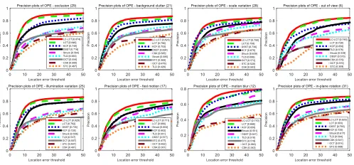
Fig. 8. Precision plots on some attribute categories.

process. Our latent constrains are only added to the context tracker (i.e., no change to the appearance tracker). Parameter settings follow [22]. The results are shown in Fig. 7

The LC-LCT and LCT achieve 78.2% and 76.8% based on the average success rate, while the KCF and DSST trackers respectively achieve 67.4% and 67.8%. In terms of precision, LC-LCT and LCT respectively achieve 86.5% and 84.8% when the threshold is set to 20. LC-LCT consistently obtains much higher tracking performance than KCF (74.0%), DSST (73.7%), Struck (65.6%) and TLD (60.8%). We also observe that LC-LCT exhibits very good performance on some at-tribute categories, such as occlusion, illumination variation, out of view, etc. On the subset of occlusion, LC-LCT is about 3% higher than LCT (87.4% vs 84.6%). These results are presented in Fig.8. In terms of tracking speed, LCT processes 29.67 frames per second (FPS), while LC-LCT has a processing rate of 25.43 FPS. Therefore, the proposed LC-LCT only has a minuscule frame rate drop as compared to the original LCT, yet is still able to achieve real-time processing. These results confirm that the latent constraint contributes to our tracker and enables it to perform better than the state-of-the-art methods.

VI. CONCLUSIONS

In this paper, we have proposed the latent constrained correlation filters (LCCF) and introduced a subspace ADMM algorithm to solve the new learning model. The theoretical analysis reveals that the new subspace ADMM is much faster than the original ADMM in terms of the convergence speed. The experimental results have shown consistent advantages over the state-of-the-arts when applying LCCF to several com-puter vision applications including eye detection, car detection and object tracking. In future work, we will incorporate the latent constraint in deep learning frameworks, and explore other applications such as action recognition [37], image retrieval [9], [18] and visual saliency detection [38], [32].

REFERENCES

[1] S. M. Bileschi. Streetscenes: Towards scene understanding in still images. Technical report, MASSACHUSETTS INST OF TECH CAM-BRIDGE, 2006.

(10)

[3] D. S. Bolme, B. A. Draper, and J. R. Beveridge. Average of synthetic exact filters. InComputer Vision and Pattern Recognition, 2009. CVPR 2009. IEEE Conference on, pages 2105–2112. IEEE, 2009.

[4] S. Boyd, N. Parikh, E. Chu, B. Peleato, and J. Eckstein. Distributed optimization and statistical learning via the alternating direction method of multipliers.Foundations and TrendsR in Machine Learning, 3(1):1– 122, 2011.

[5] G. Cabanes and Y. Bennani. Learning topological constraints in self-organizing map. Neural Information Processing. Models and Applica-tions, pages 367–374, 2010.

[6] M.-W. Chang, L. Ratinov, and D. Roth. Guiding semi-supervision with constraint-driven learning. InACL, pages 280–287, 2007.

[7] M. Danelljan, G. H¨ager, F. Khan, and M. Felsberg. Accurate scale esti-mation for robust visual tracking. InBritish Machine Vision Conference, Nottingham, September 1-5, 2014. BMVA Press, 2014.

[8] M. Danelljan, F. Shahbaz Khan, M. Felsberg, and J. Van de Weijer. Adaptive color attributes for real-time visual tracking. InProceedings of the IEEE Conference on Computer Vision and Pattern Recognition, pages 1090–1097, 2014.

[9] Y. Guo, G. Ding, L. Liu, J. Han, and L. Shao. Learning to hash with optimized anchor embedding for scalable retrieval. IEEE Transactions on Image Processing, 26(3):1344–1354, 2017.

[10] S. Hare, A. Saffari, and P. H. S. Torr. Struck: Structured output tracking with kernels. InInternational Conference on Computer Vision, pages 263–270, 2012.

[11] J. F. Henriques, R. Caseiro, P. Martins, and J. Batista. Exploiting the circulant structure of tracking-by-detection with kernels. InEuropean conference on computer vision, pages 702–715. Springer, 2012. [12] J. F. Henriques, R. Caseiro, P. Martins, and J. Batista. High-speed

tracking with kernelized correlation filters.IEEE Transactions on Pattern Analysis and Machine Intelligence, 37(3):583–596, 2015.

[13] C. F. Hester and D. Casasent. Multivariant technique for multiclass pattern recognition.Applied Optics, 19(11):1758–1761, 1980. [14] Z. Kalal, J. Matas, and K. Mikolajczyk. Pn learning: Bootstrapping

binary classifiers by structural constraints. In Computer Vision and Pattern Recognition (CVPR), 2010 IEEE Conference on, pages 49–56. IEEE, 2010.

[15] H. Kiani Galoogahi, T. Sim, and S. Lucey. Multi-channel correlation fil-ters. InProceedings of the IEEE International Conference on Computer Vision, pages 3072–3079, 2013.

[16] H. Kiani Galoogahi, T. Sim, and S. Lucey. Correlation filters with limited boundaries. InProceedings of the IEEE Conference on Computer Vision and Pattern Recognition, pages 4630–4638, 2015.

[17] A. Krogh and J. Vedelsby. Neural network ensembles, cross validation, and active learning. In Advances in neural information processing systems, pages 231–238, 1995.

[18] Z. Lin, G. Ding, J. Han, and J. Wang. Cross-view retrieval via probability-based semantics-preserving hashing. IEEE Transactions on Cybernetics, 47(12):4342–4355, 2017.

[19] T. Liu, G. Wang, and Q. Yang. Real-time part-based visual tracking via adaptive correlation filters. InProceedings of the IEEE Conference on Computer Vision and Pattern Recognition, pages 4902–4912, 2015. [20] D. G. Lowe. Object recognition from local scale-invariant features. In

Computer vision, 1999. The proceedings of the seventh IEEE interna-tional conference on, volume 2, pages 1150–1157. Ieee, 1999. [21] C. Ma, J.-B. Huang, X. Yang, and M.-H. Yang. Hierarchical

con-volutional features for visual tracking. In Proceedings of the IEEE International Conference on Computer Vision, pages 3074–3082, 2015. [22] C. Ma, X. Yang, C. Zhang, and M.-H. Yang. Long-term correlation tracking. InProceedings of the IEEE Conference on Computer Vision and Pattern Recognition, pages 5388–5396, 2015.

[23] A. Mahalanobis, B. V. Kumar, and D. Casasent. Minimum average correlation energy filters.Applied Optics, 26(17):3633–3640, 1987. [24] A. Mahalanobis, B. V. Kumar, and S. Sims. Distance-classifier

correlation filters for multiclass target recognition. Applied Optics, 35(17):3127–3133, 1996.

[25] A. Mahalanobis, B. V. Kumar, S. Song, S. Sims, and J. Epperson. Unconstrained correlation filters. Applied Optics, 33(17):3751–3759, 1994.

[26] A. Rodriguez, V. N. Boddeti, B. V. Kumar, and A. Mahalanobis. Maximum margin correlation filter: A new approach for localization and classification.IEEE Transactions on Image Processing, 22(2):631–643, 2013.

[27] M. Tang and J. Feng. Multi-kernel correlation filter for visual tracking. In Proceedings of the IEEE International Conference on Computer Vision, pages 3038–3046, 2015.

[28] S. J. Wright and J. Nocedal. Numerical optimization.Springer Science, 35(67-68):7, 1999.

[29] Y. Wu, J. Lim, and M.-H. Yang. Online object tracking: A benchmark.

InProceedings of the IEEE conference on computer vision and pattern recognition, pages 2411–2418, 2013.

[30] L. Yang, C. Chen, H. Wang, B. Zhang, and J. Han. Adaptive multi-class correlation filters. InPacific Rim Conference on Multimedia, pages 680– 688. Springer, 2016.

[31] R. Yao, S. Xia, F. Shen, Y. Zhou, and Q. Niu. Exploiting spatial structure from parts for adaptive kernelized correlation filter tracker.IEEE Signal Processing Letters, 23(5):658–662, 2016.

[32] X. Yao, J. Han, D. Zhang, and F. Nie. Revisiting co-saliency detection: a novel approach based on two-stage multi-view spectral rotation co-clustering,. IEEE Transactions on Image Processing, 26(7):3196–3209, 2017.

[33] B. Zhang, Z. Li, X. Cao, Q. Ye, C. Chen, L. Shen, A. Perina, and R. Ji. Output constraint transfer for kernelized correlation filter in tracking. IEEE Transactions on Systems, Man, and Cybernetics: Systems, 47(4):693–703, 2017.

[34] B. Zhang, Z. Li, A. Perina, A. Del Bue, V. Murino, and J. Liu. Adaptive local movement modeling for robust object tracking. InIEEE Trans. Circuits Syst. Video Techn., volume 1, pages 1515–1526. IEEE, 2017. [35] B. Zhang, A. Perina, Z. Li, V. Murino, J. Liu, , and R. Ji.

Bound-ing multiple gaussians uncertainty with application to object trackBound-ing. International Journal of Computer Vision, 118(3):364–379, 2016. [36] B. Zhang, A. Perina, V. Murino, and A. Del Bue. Sparse representation

classification with manifold constraints transfer. InProceedings of the IEEE conference on computer vision and pattern recognition, pages 4557–4565, 2015.

[37] B. Zhang, Y. Yang, C. Chen, L. Yang, J. Han, and L. Shao. Action recognition using 3d histograms of texture and a multi-class boosting. IEEE Transactions on Image Processing, 26(10):4648–4660, 2017. [38] D. Zhang, J. Han, L. Jiang, S. Ye, and X. Chang. Revealing event

saliency in unconstrained video collection.IEEE Transactions on Image Processing, 26(4):1746–1758, 2017.

[39] K. Zhang, Q. Liu, Y. Wu, and M.-H. Yang. Robust visual tracking via convolutional networks without training. IEEE Transactions on Image Processing, 25(4):1779–1792, 2016.

[40] L. Zhang, D. Bi, Y. Zha, S. Gao, H. Wang, and T. Ku. Robust and fast visual tracking via spatial kernel phase correlation filter. Neurocomputing, 204:77–86, 2016.

Appendix I: Convergence of SADMM

To prove the convergence of SADMM, we set F(ˆh) =

1 2

B

P

i=1

||yiˆ −Xiˆ h||ˆ 2

2 +

λ

2||h||ˆ 2

2. Then Eq. 7 can be rewritten

as:

Lσ(ˆh) =F(ˆh) +

σ

2k

ˆ

h−gkˆ 2_. ₍₃₂₎

We set hˆ∗ as the saddle point for the objective mentioned above. Considering the case ε =khˆt+1₋_hˆt_k2 _{as shown in}

Algorithm 1,hˆt+1 _minimizes

F(ˆht+1) +σ

t

2 k

ˆ

hk+1−ˆgtk2₊σt

2k

ˆ

ht+1−hˆtk2_. ₍₃₃₎

Sincegˆ = ˆh, Eq.(33) is rewritten as:

Lσ(ˆh) =F(ˆht+1) +σtkhˆt+1−gˆtk2, (34)

and the derivative of Eq. (34) is:

∂F(ˆht+1) + 2σt(ˆht+1−gˆt), (35)

which can also be considered as the derivative of Eq.(36):

F(ˆh) + 2σt(ˆht+1−gˆt)ˆh. (36)

We have:

F(ˆht+1) + 2σt(ˆht+1−gˆt)ˆht+1

≤F(ˆh∗) + 2σt(ˆht+1−gˆt)ˆh∗ (37)

and obtain:

(11)

In addition, based on Eq.(32), we have:

F(ˆht+1)+σ

t

2 k

ˆ

ht+1−gˆtk2_≥_F_(ˆ_h∗₎₊σt

2 σ

t_k_h_ˆ∗₋_g_ˆt_k2_.

(39)

Since ˆh∗ is the saddle point for our problem, we have:

F(ˆh∗)−F(ˆht+1)≤ σ t

2 ∗(k

ˆ

ht+1−ˆgtk2_{− k}_h_ˆ∗₋_g_ˆt_k2₎_. ₍₄₀₎

From Eq. (38) and Eq. (40), we get:

−4khˆt+1−hˆ∗k2_{+ 4(ˆ}_h∗₋_ˆ_gt_)(ˆ_h∗₋_hˆt+1₎

+khˆt+1−gˆtk2− khˆ∗−gˆtk2≥0. (41)

where we also used 4(ˆht+1₋_hˆ∗_{+ ˆ}_h∗₋_ˆ_gt_)(ˆ_h∗₋_hˆt+1₎_to

change the right part of Eq. (38). And then we have:

khˆt+1−gˆtk2=khˆt+1−hˆ∗k2+khˆ∗−gˆtk2

+ 2(ˆht+1−hˆ∗)(ˆh∗−gˆt), (42)

we have:

−4khˆt+1−hˆ∗k2_{+ 4(ˆ}_h∗₋_g_ˆt_)(ˆ_h∗₋_hˆk+1₎

+khˆt+1−gˆtk2+khˆt+1−gˆtk2

− khˆ∗−gˆtk2_{− k}_h_ˆt+1₋_ˆ_gt_k2

=−4khˆt+1−hˆ∗k2_{+ 2}_k_h_ˆt+1₋_h_ˆ∗_k2_{+ 2}_k_h_ˆ∗₋_g_ˆt_k2

−khˆ∗−gˆtk2_{− k}_h_ˆt+1₋_g_ˆt_k2_≥₀_.

(43)

Therefore we obtain:

−2khˆt+1−hˆ∗k2₊_k_h_ˆ∗₋_ˆ_gt_k2_{− k}_h_ˆt+1₋_ˆ_gt_k≥₀ ₍₄₄₎

Again, usinggˆ = ˆh, we have:

khˆt+1−hˆ∗k2_≤1

2k

ˆ

h∗−hˆtk2₋1

2k

ˆ

ht+1−ˆgtk2_. ₍₄₅₎

Compared to [4], our method is more efficient than ADMM in terms of convergence speed.

Appendix II: Kernelized correlation filters (KCF)

We briefly review the KCF algorithm. Based on the input image of xof M ×N pixels, in the spatial domain, KCF is described as

min

h

X

i

ξ_i2

subject to yi−hTφ(xi) =ξi ∀i; ||h|| ≤C.

(46)

In Eq. (46), xi is the circular samples of image x. y representing a Gaussian output andξdenoting a slack variable, are vectors. Therefore, yi andξi in Eq. (46) are scalars.φ(.) (later φi) refers to the nonlinear kernel function, and C is a small constant. Then, we have

Lp=

M×N

X

i=1

ξi2+ M×N

X

i=1

θi(yi−hTφi−ξi) +λ(||h||2−C2),

(47) Using KKT conditions θi = 2ξi, h = P_iM×N ₂θ_λiφi and settingαi= ₂θ_λi, solvinghwill be converted to solving a dual

variableαin a dual space. Pluggingαback into Eq.(47), we formulate a new maximizing objective functionE(α):

E(α) =−λ2

M×N

X

i=1

α2_i+2λ

M×N

X

i=1

αiyi−λ M×N

X

i,j=1

αiαjKi,j−λC2,

(48) whereKis a kernel matrix. Then, the solution is

α= (K+λI)−1y. (49)

According to the properties of the cyclic matrix, Eq. (49) is transformed into the Fourier domain to speed up the calculation based on Fast Fourier Transform (FFT). Then, we haveαˆ as:

ˆ

α= (Kxx+λI)−1yˆ, (50)

whereKxx _{refers to the first row of}_K.

Baochang Zhangis currently an associate professor with Beihang University, Beijing, China. His research interests include pattern recognition, machine learning, face recognition, and wavelets.

Shangzhen Luan received the B.S. degrees in automation from Beihang University. His research interests include signal and image processing, pattern recognition and computer vision

Chen Chenis currently a Postdoctoral Fellow with the Center for Research in Computer Vision, University of Central Florida, Orlando, FL, USA. His research interests include compressed sensing, signal and image processing, pattern recognition, and computer vision.

Jungong Han is currently a tenured faculty member with the School of Computing and Communications at Lancaster University, UK. His research interestes include video analysis, computer vision and artificial intelligence.

Wei Wangis currently an Associate Professor with the School of Automation Science and Electrical Engineering at Beihang University and supported by BUAA Young Talent Recruitment Program.

Alessandro Perina is currently a data scientist at Microsoft Corporation, Redmond, WA, USA. His area of expertise lies in machine learning, statistics and applications, particularly in probabilistic graphical models, unsupervised learning, and optimization algorithms.