Weak regularity and finitely forcible graph limits

warwick.ac.uk/lib-publications

Original citation:

Cooper, Jacob W., Kaiser, Tomas, Králʼ, Daniel and Noel, Jonathan (2018) Weak regularity and finitely forcible graph limits. Transactions of the American Mathematical Society . doi:10.1090/tran/7066

Permanent WRAP URL:

http://wrap.warwick.ac.uk/81519

Copyright and reuse:

The Warwick Research Archive Portal (WRAP) makes this work by researchers of the University of Warwick available open access under the following conditions. Copyright © and all moral rights to the version of the paper presented here belong to the individual author(s) and/or other copyright owners. To the extent reasonable and practicable the material made available in WRAP has been checked for eligibility before being made available.

Copies of full items can be used for personal research or study, educational, or not-for-profit purposes without prior permission or charge. Provided that the authors, title and full

bibliographic details are credited, a hyperlink and/or URL is given for the original metadata page and the content is not changed in any way.

Publisher’s statement:

First published in Transactions of the American Mathematical Society [28-02-2018] published by the American Mathematical Society. © 2018 American Mathematical Society.

A note on versions:

The version presented here may differ from the published version or, version of record, if you wish to cite this item you are advised to consult the publisher’s version. Please see the ‘permanent WRAP URL’ above for details on accessing the published version and note that access may require a subscription.

Weak regularity and finitely forcible graph limits

∗

Jacob W. Cooper

Tom´aˇs Kaiser

Daniel Kr´al’

Jonathan A. Noel

Abstract

Graphons are analytic objects representing limits of convergent sequences of graphs. Lov´asz and Szegedy conjectured that every finitely forcible graphon, i.e. any graphon determined by finitely many graph densities, has a simple structure. In particular, one of their conjectures would imply that every finitely forcible graphon has a weak ε-regular partition with the number of parts bounded by a polynomial in ε−1_{. We construct a finitely forcible graphon W such that the number of parts}

in any weak ε-regular partition of W is at least exponential in ε−2/25 log∗ε−2. This bound almost matches the known upper bound for graphs and, in a certain sense, is the best possible for graphons.

1

Introduction

The theory of combinatorial limits has recently attracted a significant amount of attention. This line of research was sparked by limits of dense graphs [7–9,32], which we focus on here, followed by limits of other structures, e.g. permutations [22,23,28], sparse graphs [5,14] and partial orders [25]. Methods related to combinatorial limits have led to substantial results in many areas of mathematics and computer science, particularly in extremal combinatorics. For example, the notion of flag algebras, which is strongly related to combinatorial limits, resulted in progress on many important problems in extremal combinatorics [1–4, 19–21,

∗_{The work of the first and third authors leading to this invention has received funding from the European}

Research Council under the European Union’s Seventh Framework Programme (FP7/2007-2013)/ERC grant agreement no. 259385.

†_{Department of Computer Science, University of Warwick, Coventry CV4 7AL, UK. E-mail:}

[email protected].

‡_{Department of Mathematics, Institute for Theoretical Computer Science (CE-ITI) and the European}

Centre of Excellence NTIS (New Technologies for the Information Society), University of West Bohemia, Univerzitn´ı 8, 306 14 Plzeˇn, Czech Republic. E-mail: [email protected]. This author was supported by the grant GA14-19503S (Graph coloring and structure) of the Czech Science Foundation.

§_{Mathematics Institute, DIMAP and Department of Computer Science, University of Warwick,}

Coven-try CV4 7AL, UK. E-mail: [email protected]. The work of this author was also supported by the Engineering and Physical Sciences Research Council Standard Grant number EP/M025365/1.

26, 27, 34–38]. Theory of combinatorial limits also provided a new perspective on existing concepts in other areas, e.g. property testing algorithms in computer science [16, 24, 33].

A convergent sequence of dense graphs can be represented by an analytic object called a graphon. Let d(H, W) be the density of a graph H in a graphon W (a formal definition is given in Section 2). A graphon W is said to be finitely forcible if it is determined by finitely many graph densities, i.e. there exist graphs H1, . . . , Hk and reals d1, . . . , dk such

that W is the unique graphon with d(Hi, W) = di. Finitely forcible graphons appear in

many different settings, one of which is in extremal combinatorics. It is known that if a graphon is finitely forcible, then it is the unique graphon which minimizes a fixed finite linear combination of subgraph densities, i.e. finitely forcible graphons are extremal points of the space of all graphons. The following conjecture [31, Conjecture 7] claims that the converse is also true.

Conjecture 1. LetH1, . . . , Hk be finite graphs and α1, . . . , αk reals. There exists a finitely

forcible graphon W that minimizes the sum

k P i=1

αid(Hi, W).

Finitely forcible graphons are also related to quasirandomness in graphs as studied e.g. by Chung, Graham and Wilson [10], R¨odl [39], and Thomason [40, 41]. In the language of graph limits, results on quasirandom graphs state that every constant graphon is finitely forcible. A generalization of this statement was proven by Lov´asz and S´os [30]: every step graphon (i.e. a multipartite graphon with a finite number of parts and uniform edge densities between its parts) is finitely forcible.

In [31], Lov´asz and Szegedy carried out a more systematic study of finitely forcible graphons. The examples of finitely forcible graphons that they constructed led to a belief that finitely forcible graphons must have a simple structure. To formalize this, they intro-duced the (topological) space T(W) of typical vertices of a graphon W and conjectured the following [31, Conjectures 9 and 10].

Conjecture 2. The space of typical vertices of every finitely forcible graphon is compact.

Conjecture 3. The space of typical vertices of every finitely forcible graphon has a finite dimension.

Both conjectures were disproved through counterexample constructions in [17, 18].

Conjecture 3 is a starting point of our work. Analogously to weak regularity of graphs, every graphon has a weakε-regular partition with at most 2O(ε−2) parts. (See Section 3 for the necessary definitions.) If the space of typical vertices of a graphon is equipped with an appropriate metric, then its Minkowski dimension is linked to the number of parts in its weak regular partitions. In particular, if its Minkowski dimension is d, then the graphon has weakε-regular partitions with O ε−d

parts. Consequently, if Conjecture 3 were true, the number of parts of a weak ε-regular partitions of a finitely forcible graphon would be bounded by a polynomial of ε−1_{. The number of parts in weak ε-regular partitions of a}

graphon constructed in [17] as a counterexample to Conjecture 3 is 2Θ(log2_ε−1₎

superpolynomial inε−1_{, but is much smaller than the general upper bound of 2}O(ε−2

). We construct a finitely forcible graphon almost matching the upper bound.

Theorem 1. There exist a finitely forcible graphon W and positive reals εi tending to 0

such that every weak εi-regular partition of W has at least 2 Ω

ε−_i2/25 log∗ε −2

i

parts.

As pointed out to us by Jacob Fox, there is no graphon (finitely forcible or not) matching the upper bound 2O(ε−2) for infinitely many values of ε tending to 0. In light of this, Theorem 1 is almost the best possible.

Proposition 2. There exist no graphon W, a positive real c and positive reals εi tending

to 0 such that every weak εi-regular partition of W has at least 2cε −2

i parts.

The proof of this proposition is sketched at the end of Section 3.

We will refer to the graphon W from Theorem 1 as the ˇSvejk graphon. ˇSvejk is the name of a famous (and fictitious) brave Czech soldier and, more importantly for us, it is the name of the restaurant where we usually ate lunch during our work on this subject while three of us were visiting the University of West Bohemia in Pilsen.

2

Graph limits

We now introduce notions related to graphons and convergent sequences of graphs. The

densityof a graphHinG, which is denoted byd(H, G), is the probability that|H|randomly chosen vertices ofGinduce a subgraph isomorphic toH, where|H|is the order (the number of vertices) of H. A sequence of graphs (Gn)n∈N with the number of their vertices tending to infinity isconvergentif the sequence d(H, Gn) converges for every graphH. Note that if Gn has o(|Gn|2) edges, then the sequence (Gn)n∈N is convergent for trivial reasons. Hence, this notion of graph convergence is of interest for sequences of dense graphs, i.e. graphs with Ω(|Gn|2_{) edges.}

A convergent sequence of dense graphs can be represented by an analytic object called a graphon. A graphon W is a measurable function from [0,1]2 _{to [0,1] that is symmetric,}

i.e. it holds that W(x, y) = W(y, x) for every x, y ∈ [0,1]. The points in [0,1] are often referred to as the vertices of the graphon W.

If W is a graphon, then a W-random graph of order k is obtained by sampling k

random points x1, . . . , xk ∈ [0,1] uniformly and independently, and joining the i-th and

the j-th vertex by an edge with probability W(xi, xj). The density of a graph H in a

graphon W is the probability that a W-random graph of order |H| is isomorphic to H. If (Gn)n∈N is a convergent sequence of graphs, then there exists a graphon W such that

d(H, W) = lim

n→∞d(H, Gn) for every graph H [32]. This graphon can be viewed as the limit

of the sequence (Gn)n∈N. On the other hand, a sequence ofW-random graphs of increasing orders is convergent with probability one and its limit is the graphon W.

Two graphons W1 and W2 are weakly isomorphic if there exist measure preserving

almost every pair (x, y)∈[0,1]2_{. If two graphons W}

1 and W2 are weakly isomorphic, then d(H, W1) = d(H, W2) for every graph H. The converse is also true [6]: if two graphons W1 and W2 satisfy that d(H, W1) = d(H, W2) for every graph H, then W1 and W2 are

weakly isomorphic. Hence, the limit of a convergent sequence of graphs is unique up to weak isomorphism. We finish with giving a formal definition of a finitely forcible graphon: a graphonW isfinitely forcible if there exist graphsH1, . . . , Hk such that if a graphonW′

satisfies that d(Hi, W′) = d(Hi, W) for i = 1, . . . , k, then d(H, W′) = d(H, W) for every

graph H.

3

Weak regular partitions

In this section, we recall some basic concepts related to weak regularity for graphs and graphons and cast the lower bound construction of Conlon and Fox from [11] in the language of graphons. Since we do not use any other type of regularity partition, we will just say “regular” instead of “weak regular” in what follows.

We start with defining the notion for graphs. If Gis a graph and Aand B two subsets of its vertices, let e(A, B) be the number of edges uv such that u ∈ A and v ∈ B. A partition of a vertex set V(G) of a graph G into subsets V1, . . . , Vk is said to be ε-regular

if it holds that

e(A, B)− X i,j∈[k]

e(Vi, Vj) |Vi||Vj|

|Vi∩A||Vj∩B|

≤ε|V(G)|2

for every two subsets A and B of V(G). It is known that for every ε > 0, there exists

k0 ≤ 2O(ε −2

) (which depends on ε only) such that every graph has an ε-regular partition with at most k0 parts [15]. This dependence of k0 on ε is best possible up to a constant

factor in the exponent as shown by Conlon and Fox [11].

We now define the analogous notion for graphons. LetW : [0,1]2 _{→[0,1] be a graphon.}

IfA and B are two measurable subsets of [0,1], then the density dW(A, B) between A and B is defined to be

dW(A, B) = Z

A×B

W(x, y) dxdy.

We will omit W in the subscript if the graphon W is clear from the context. Note that it always holds thatd(A, B)≤ |A||B|where|X| is the measure of a set X. We would like to mention that the density between A and B is often defined in a normalized way, i.e. it is defined to be d_|(_AA,B_||B|), but this is not the case in this paper.

A partition of [0,1] into measurable non-null sets U1, . . . , Uk is said to be ε-regular if it

holds that

d(A, B)− X i,j∈[k]

d(Ui, Uj)

|Ui||Uj| |Ui∩A||Uj ∩B|

for every two measurable subsets A and B of [0,1]. The upper bound proof translates directly from graphs to graphons and so we get that for every ε, there exists k0 ≤2O(ε

−2₎

such that every graphon has an ε-regular partition with at most k0 parts. Likewise, the

example of Conlon and Fox from [11] can be used to obtain a step-graphon Wε such that

every ε-regular partition of Wε has at least 2Ω(ε −2

) parts. However, the construction is probabilistic and the description ofWε is thus not explicit. Based on this construction, we

will define an explicit graphon Wm

CF which has similar properties as Wε for ε ≈m−1/2. In

fact, a Wm

CF-random graph of order 2αm for some α close to 0 is the graph constructed by

Conlon and Fox in [11].

Fix an integer m. The graphon Wm

CF is a step graphon that consists of 2m parts of

equal size. Each of the parts is associated with a vector u ∈ {−1,+1}m_{. The part of the}

graphon Wm

CF corresponding to vectors u and u′ is constantly equal to trunc

1 2 +

hu,u′_i 4m1/2

where trunc (x) is equal to x if x ∈ [0,1], it is equal to 0 if x < 0 and to 1 if x > 1. In other words, the operator trunc (·) replaces values smaller than 0 or larger than 1 with 0 and 1, respectively. Observe that d([0,1],[0,1]) = 1/2 by symmetry. Using the Chernoff bound, one can show that the measure of the points (x, y) with 0< W(x, y)<1 is at least 1−2e−2 _>1/2.

It would be possible to relate the proof presented in [11] to arguments on regular partitions of graphons. However, the probabilistic nature of the construction would make this technical and obfuscate some simple ideas. Because of this, and to keep the paper self-contained, we decided to present a direct proof following the lines of the reasoning given in [11].

Theorem 3. If m≥25andε < 1

214_m1/2, then every ε-regular partition of the graphon WCFm

has at least 2m/4 _parts.

Proof. Fix an integer m≥25. Let V_i− be the vertices of Wm

CF in the parts associated with

vectors u whose i-th coordinate equals −1. Similarly, V_i+ are the vertices of Wm

CF in the

parts associated with vectors u whose i-th coordinate equals +1. Suppose that Wm

CF has an ε-regular partition U1, . . . , Uk with ε < 2−14m−1/2 and k <

2m/4_{. We say that a part U}

t issmall if |Ut| ≤2−m/3. Note that the sum of the measures of

the small parts is at most k·2−m/3 _{≤1/2. For every t∈[k], set}

St= X

i∈[m]

|Ut∩Vi−| · |Ut∩Vi+|. (1)

If v ∈ {−1,+1}m_{, then the number of vectors v}′ _{∈ {−1,+1}}m _{such that v and v}′ _{differ in}

at mostm/16 coordinates is at most 2m−₁₂₈49m_≤22m/3−1 _{using the Chernoff bound and the}

fact thatm≥25. Hence, for everyv ∈ {−1,+1}m_{, the measure of the vertices in the parts}

associated with vectors that differ fromv in at mostm/16 coordinates is at most 2−m/3_/2.

Consequently, if Ut is not small, then each vertex of Ut contributes to the sum (1) by at

least ₁₆m |Ut| −2−m/3_/2

≥m|Ut|/32. We conclude that St≥ |Ut|2m/32 if Ut is not small.

We say that the pair (i, t)∈ [m]×[k] is useful if min{|Ut∩Vi−|,|Ut∩Vi+|} ≥ |Ut|/64.

each term in the sum (1) is at most |Ut|2_{/4 and it is at most |Ut|}2_{/64 if (i, t) is not useful,}

it follows that St≤ |Ut|2(Mt/4 +m/64). We conclude thatMt ≥m/16 unless Ut is small

(recall that St ≥ |Ut|2m/32 if Ut is not small). Since the sum of the measures of the parts

that are not small is at least 1/2, we obtain that

X

t∈[k]

Mt|Ut| ≥m/32 . (2)

In particular, there exists i0 ∈[m] such that the sum of the measure of parts Ut such that

the pair (i0, t) is useful is at least 1/32. Fix such an index i0 for the rest of the proof.

LetA− _{be any measurable subset ofV}−

i0 such that|A

−_{∩Ut|=|Ut|/64 if (i}

0, t) is useful,

and |A−_∩U

t| = 0 otherwise. Similarly, let A+ be any measurable subset of Vi+0 such that |A+_{∩Ut| =|Ut|/64 if (i}

0, t) is useful, and |A+∩Ut|= 0 otherwise. Such sets A− and A+

exist because min{|Ut∩Vi−0 |,|Ut ∩V

+

i0|} ≥ |Ut|/64 for every t such that (i0, t) is useful.

Note that the sets A− _{and A}+ _{have the same measure and the choice of i}

0 implies this

measure is at least 1/2048 = 2−11_.

Let B =V_i−₀. Since the partition U1, . . . , Uk is ε-regular, we get that

d(A+, B)− X i,j∈[k]

d(Ui, Uj)

|Ui||Uj| |Ui∩A +_||U

j∩B|

≤ ε

and that

d(A−, B)− X i,j∈[k]

d(Ui, Uj) |Ui||Uj|

|Ui∩A−||Uj ∩B|

≤ε.

Since |A− _{∩ Ut| = |A}+ _{∩Ut| for every t ∈ [k], we infer that |d(A}−_{, B) −d(A}+_{, B)| ≤}

2ε <2−13_m−1/2_{. On the other hand, the choices of A}−_,A+ _{and B imply thatd(A}−_{, B) =}

(1/2 +m−1/2_/4)|A−_{||B| and d(A}+_{, B) = (1/2−m}−1/2_/4)|A+_{||B|. In particular, it holds}

that

|d(A−, B)−d(A+, B)|= m

−1/2_(|A−_|+|A+_|)|B|

4 ≥2

−13_·m−1/2 _.

This contradicts the fact thatU1, . . . , Ukis anε-regular partition ofWCFm withε <2−14m−1/2

and k < 2m/4_.

At first sight, it might seem natural to consider the limit of the sequence of the graphons

Wm

CF,m∈N, as a candidate for a graphon with no regular partitions with few parts. It can

be shown that the sequence of Wm

CF, m∈N, is convergent, however, its limit is (somewhat

surprisingly) the graphon that maps every (x, y) ∈ [0,1]2 _{to 1/2, which has an ε-regular}

partition with one part for every ε.

Suppose that there exists a graphon W and εi →0 as in the proposition. We can assume

that εi+1 ≤ εi/2 for every i ∈ N. We start with a trivial partition into a single part and

keep refining it until it becomes ε1-regular; let k1 be the number of steps made. We then

continue with refining until it becomes ε2-regular and let k2 ≥ k1 be the total number of

steps made till this point. We continue this procedure and defineki,i≥3, in the analogous

way. Setting k0 = 0, we conclude that the mean square density afterkm steps is at least

m X

i=1

(ki−ki−1)ε2i > m X

i=1

ki ε2i −ε2i+1

≥ m X

i=1

3 4kiε

2 i .

However, eachkimust be at leastcε−2i by the assumption of the proposition (otherwise,W

would have a weak εi-regular partition with fewer than 2cε −2

i parts). Consequently, after

m=₄ 3c

+ 1 steps, the mean square density exceeds one, which is impossible.

4

Definition of the ˇ

Svejk graphon

We now define the ˇSvejk graphonWS. We start with defining a tower functiont(n) :N→N

as follows:

t(n) =

1 if n= 0, and 2t(n−1) _otherwise.

Note thatt(0) = 1,t(1) = 2,t(2) = 22 _{= 4, t(3) = 2}22

= 16, t(4) = 2222

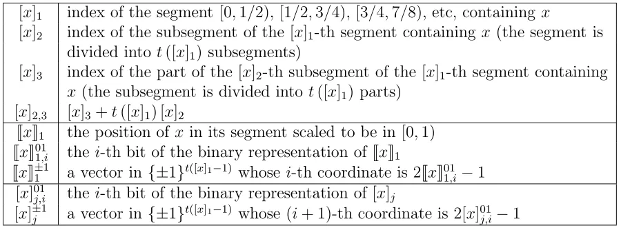
= 65536, etc. The notation that we define next is summarized in Table 1. Forx∈[0,1), we define [x]1

to be the smallest integer k such that x <1−2−k_{. In particular, [x]}

1 = 1 iff x ∈[0,1/2),

[x]1 = 2 iffx∈[1/2,3/4), [x]1 = 3 iffx∈[3/4,7/8), etc. This allows us to view the interval

[0,1) as split into segments [0,1/2), [1/2,3/4), [3/4,7/8), etc. and [x]1 is the index of the

segment containingx(numbered from one). We then defineJxK1 to be (x+21−[x]1−1)·2[x]1,

i.e. JxK1 is the position of x in the [x]1-th segment if the [x]1-th segment is scaled to the

unit interval.

Next, we let [x]2 equal ⌊JxK1 ·t([x]1)⌋. In other words, if the [x]1-th segment of [0,1)

is divided into t([x]1) parts of the same length 2−[x]1/t([x]1), then [x]2 is the index of

the part containing x if the parts are numbered from 0. We refer to these parts of the segments as subsegments. Analogously, we let [x]3 be the index of the part containing x

when the [x]2-th subsegment of the [x]1-th segment is divided into t([x]1) parts of length

2−[x]1_/t([x]

1)2, where the parts are numbered from 0. Define [x]2,3 to be [x]3+t([x]1) [x]2.

Note that [x]2,3 can also be viewed as the part containing x when the [x]1-th segment is

divided into t([x]1)2 parts of length 2−[x]1/t([x]1)2, and that [x]3 is equal to [x]2,3 reduced

modulo t([x]1).

Fori≥1, letJxK01

1,idenote thei-th bit in the binary representation ofJxK1. For example,

if JxK1 = 0.375 = .011 in binary, then JxK011,1 = 0, JxK011,2 = JxK011,3 = 1 and JxK011,i = 0 for i ≥ 4. We let JxK±1

1 denote the vector in {±1}t([x]1−1) whose i-th coordinate is equal to

2JxK01

[x]1 index of the segment [0,1/2), [1/2,3/4), [3/4,7/8), etc, containing x

[x]2 index of the subsegment of the [x]1-th segment containing x(the segment is

divided into t([x]1) subsegments)

[x]3 index of the part of the [x]2-th subsegment of the [x]1-th segment containing x (the subsegment is divided into t([x]1) parts)

[x]2,3 [x]3+t([x]1) [x]2

JxK1 the position of x in its segment scaled to be in [0,1) JxK01

1,i the i-th bit of the binary representation of JxK1

JxK±1₁ a vector in {±1}t([x]1−1) _{whose i-th coordinate is 2JxK}01

1,i−1

[x]01

j,i the i-th bit of the binary representation of [x]j

[x]±1_j a vector in {±1}t([x]1−1) _{whose (i+ 1)-th coordinate is 2[x]}01 j,i−1

Table 1: The notation used in the definition of the ˇSvejk graphon.

For j ∈ {2,3} and i ≥ 0, let [x]01

j,i denote the i-th bit in the binary representation of

[x]j. For example, if [x]j = 5 = 20+ 22, then [x]01j,0 = [x]01j,2 = 1, [x]01j,1 = 0 and [x]01j,i = 0 for i ≥3. We let [x]±1_j denote the vector in {±1}t([x]1−1) _{whose (i+ 1)-th coordinate is equal}

to 2[x]01 j,i−1.

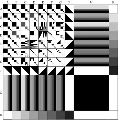
The ˇSvejk graphonWS has ten partsA,B,C,D,E, F,G,P,QandR. For simplicity,

we will define the graphon WS as a function W13 from [0,13) ×[0,13) to [0,1], and we

set WS(x, y) = W13(13x,13y). All parts of W13 except for Q have measure one and we

associate each of them with the unit interval [0,1), i.e. we view the points of those parts as points in [0,1). The remaining part Qis associated with [0,4).

We will first define the values of the graphon W13 between the pairs of the parts not

involving QandR. The graphonW13 has values zero and one on (A∪ · · · ∪G∪P)2 except

onC2_{, E}2_{,B×Dand D×B. Table 2 determines the values ofW}

13 in this zero-one case.

The values ofW13 onC2, E2 and B×D (by symmetry, this also determines the values on D×B) are defined as follows. Note that the definition uses the graphon Wm

CF analyzed in

Section 3, which was defined just before the statement of Theorem 3.

W13(x, y) =

2−2[x_]1−1

if [x]1 = [y]1, and

0 otherwise, for (x, y)∈C

2_,

W13(x, y) =

Wt([x]1−1)

CF (JxK1,JyK1) if [x]1 = [y]1, and

0 otherwise, for (x, y)∈E

2_{, and}

W13(x, y) =

t([x]1)−1 if [x]1 = [y]1, and

0 otherwise, for (x, y)∈B×D.

We have defined the values of the graphonW13 on (A∪ · · · ∪G∪P)2, i.e. between all pairs

A B C D E F G P Q R A

B

C

D

E

F

G

P

Q

R

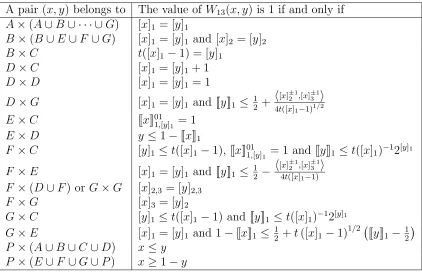
A pair (x, y) belongs to The value of W13(x, y) is 1 if and only if A×(A∪B∪ · · · ∪G) [x]1 = [y]1

B×(B∪E∪F ∪G) [x]1 = [y]1 and [x]2 = [y]2 B×C t([x]1−1) = [y]1

D×C [x]1 = [y]1+ 1 D×D [x]1 = [y]1 = 1

D×G [x]1 = [y]1 and JyK1 ≤ 1₂ + h

[x]±₂1,[x]±₃1i 4t([x]1−1)1/2

E×C JxK01

1,[y]1 = 1 E×D y ≤1−JxK1

F ×C [y]1≤t([x]1−1), JxK01_1,[y]1 = 1 andJyK1 ≤t([x]1)−12[y]1 F ×E [x]1 = [y]1 and JyK1 ≤ 1₂ − h

[x]±₂1,[x]±₃1i 4t([x]1−1) F ×(D∪F) or G×G [x]2,3 = [y]2,3

F ×G [x]3 = [y]2

G×C [y]1≤t([x]1−1) and JyK1 ≤t([x]1)−12[y]1

G×E [x]1 = [y]1 and 1−JxK1 ≤ ₂1 +t([x]1 −1)1/2 JyK1− 1₂

P ×(A∪B∪C∪D) x≤y P ×(E∪F ∪G∪P) x≥1−y

Table 2: The definition of the ˇSvejk graphon on (A∪ · · ·∪G∪P)2_{except onC}2_,E2_,B×D

The part Q is used to equalize degrees of the vertices in the parts A, . . . , G, P, i.e., to make the values

1 13

Z

[0,13)

W13(x, y) dy,

to be the same for all xfrom the same part; see Section 5 for further details on the degree of a vertex in a graphon. If x∈A∪ · · · ∪G∪P =Q∪R and y∈Q, then

W13(x, y) =

1 4



 4−

Z

Q∪R

W13(x, z) dz 

  .

It is straightforward to verify thatW13(x, y)∈[0,1] for every (x, y)∈Q∪R×Q.

The part R distinguishes the parts by vertex degrees. If y∈R, then

W13(x, y) =            

          

1/8 if x∈B, 2/8 if x∈C, 3/8 if x∈D, 4/8 if x∈E, 5/8 if x∈F, 6/8 if x∈G, 7/8 if x∈P, and

0 otherwise.

Finally, the graphon W13 is equal to 1 onQ×Q.

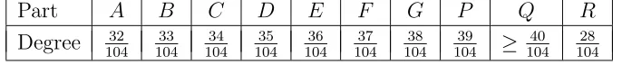
The vertices in each of the ten parts of the ˇSvejk graphon have the same degree (note thatW(x1, y) =W(x2, y) for any two verticesx1, x2 ∈Qand anyy∈[0,13)). This degree

is given in Table 3. We have not computed the degree of the vertices in the part Qexactly since it is enough to establish that this degree is larger than (and thus distinct from) the degrees of the vertices in the other parts.

Part A B C D E F G P Q R

Degree ₁₀₄32 ₁₀₄33 ₁₀₄34 ₁₀₄35 ₁₀₄36 ₁₀₄37 ₁₀₄38 ₁₀₄39 ≥ ₁₀₄40 ₁₀₄28

Table 3: The degrees of the vertices in each part of the ˇSvejk graphon.

We finish this section by establishing that the ˇSvejk graphon has no weak regular partitions with few parts.

Proposition 4. The ˇSvejk graphon WS has no weak ε-regular partition with fewer than

2t(n)/4 _{parts if ε <} 1

224+2n_t(n)1/2 and n ≥ 4. In particular, there exists a sequence of

pos-itive reals εi tending to 0 such that every weak εi-regular partition of WS has at least

2Ω

ε−_i2/25 log ∗

ε−_i2

Proof. The graphonWS contains a copy ofWCFt(n) scaled by 2−n−1/13 for everyn ∈N. Note

that a weakε-regular partition ofWS yields a weak (ε2−2n/676)-regular partition of WCFt(n)

with fewer or the same number of parts. It follows thatWS cannot have a weak ε-regular

partition with fewer than 2t(n)/4 _{parts for ε <} 1

676·214+2n_·t(n)1/2 and n ≥4 by Theorem 3.

Setting εi = ₂25+2i1_t(i)1/2, we obtain the desired sequence of εi’s. Note that

lim

i→∞

log∗ε−2_i

i = limi→∞

log∗(24i+50_t(i))

i = 1

and so t(₄i) ∈Ωε_i−2/25 log∗ε−_i2 _{as desired.}

5

Constraints

The proof that the ˇSvejk graphon is finitely forcible uses the notion of decorated constraints, which was introduced in [18] and further developed in [17]. We now present the notion following the lines of [17].

A constraintis an equality between two density expressions where adensity expression

is recursively defined as follows: a real number or a graph H are density expressions, and if D1 and D2 are two density expressions, then the sum D1+D2 and the product D1·D2

are also density expressions. The value of the density expression for a graphon W is the value obtained by substituting for each graph H its density inW.

As observed in [18], ifW is the unique graphon (up to weak isomorphism) that satisfies a finite set C of constraints, then it is finitely forcible. In particular, W is the unique graphon with densities of subgraphs appearing in C equal to their densities in W. Hence, a possible way of establishing that a graphon W is finitely forcible is providing a finite set of constraints C such that the graphon W is the unique graphon up to weak isomorphism that satisfies these constraints.

If W is a graphon, then the points of [0,1] can be viewed as vertices and we can also speak of the degree of a vertex x∈[0,1], defined as

deg_W(x) =

Z

[0,1]

W(x, y) dy.

Note that the degree is well-defined for almost every vertex of W. We will omit the subscript W when the graphon is clear from the context. A graphon W is partitioned if there existk ∈N_{and positive reals a1, . . . , ak summing to one and distinct realsd1, . . . , dk}

between 0 and 1 such that the set of vertices of W with degree di (referred to as a part of

the partitioned graphon) has measure ai. The following lemma was proven in [18].

Lemma 5. Let a1, . . . , ak be positive real numbers summing to one and let d1, . . . , dk be

distinct reals between 0 and 1. There exists a finite set of constraints C such that any graphon W satisfying C is a partitioned graphon with parts of sizes a1, . . . , ak and degrees d1, . . . , dk, and any partitioned graphon with parts of sizes a1, . . . , ak and degreesd1, . . . , dk

We now introduce a stronger type of constraints, which was also used in [17, 18]. We will refer to the constraints introduced earlier as ordinary constraintsif a distinction needs to be made. Suppose that W is a partitioned graphon with parts Ai ⊆ [0,1], i ∈ [k],

where the part Ai has measure ai and it contains vertices of degrees di. A decorated

graph is a graph with some vertices distinguished as roots and each vertex labeled with one of the parts A1, . . . , Ak; the roots of a decorated graph come with a fixed order. Two

decorated graphs are isomorphicif they have the same number of roots and there exists a bijection between their vertices that is a graph isomorphism, that maps roots to roots only while preserving their order, and that preserves vertex labels. Two decorated graphs are

compatible if the subgraphs induced by their roots are isomorphic (as decorated graphs). Adecorated constraintis a constraint where all graphs appearing in the density expressions are compatible decorated graphs. Note that decorated graphs and constraints are always defined with a particular type of a partition of a graphon (i.e. names of the parts) in mind. We now define when a graphon W satisfies a decorated constraint. Fix a decorated constraint C. Since all decorated graphs appearing in C are compatible, the roots of each of the decorated graphs appearing in C induce the same decorated graph. Let H0 be this

decorated graph and let n be the number of its vertices; note that all n vertices of H0

are roots. The decorated constraint C is satisfied if the following holds for almost every

n-tuple x1, . . . , xn of vertices of H0 such that xi belongs to the part that the i-th vertex of H0 is labeled with,W(xi, xj)>0 ifxi andxj are adjacent inH0, andW(xi, xj)<1 if they

are not adjacent: the two sides of the constraint C are equal when each decorated graph

H is substituted with the probability that a W-random graph with vertices corresponding to those of H is the decorated graph H conditioned on the root vertices being x1, . . . , xn

and inducing the graph H0 and conditioned on each of the non-root vertices chosen from

a part that it is labeled with. Note that we do not allow any permutation of vertices in this definition, i.e., the requirement is stronger than saying that the W-random graph is isomorphic to the decorated graphH0. A possible way of satisfying the constraintC is that

the measure of the n-tuples x1, . . . , xn of vertices ofH0 with the properties given above is

zero; if this is the case, the constraint C is said to be null-satisfied.

Before proceeding further, let us give an example of evaluating a decorated constraint. Consider a partitioned graphonW with two partsAand B, each of measure one half, such thatW is equal to one on A×A, to zero onB×B, and to one half on A×B. The graphon

W is depicted in Figure 2. Let H be a decorated graph with two roots that are adjacent and both labeled with A and two non-root vertices v1 and v2 that are not adjacent, both

labeled with B, v1 is adjacent to one of the roots and v2 is adjacent to both roots. The

decorated graph H is also depicted in Figure 2. If H appears in a decorated constraint and its two roots are from the part A of the graphon W, then it will be substituted with the probability 1/16 when evaluating the constraint with respect to W. Note that if we allowed isomorphisms of decorated graphs when evaluating decorated constraints, then this probability would be 2/16 because the order in that the non-root vertices are chosen would be irrelevant.

A B A

B A A

B B

=

Figure 2: An example of evaluating a decorated constraint.

A B B B

A B B B

A B B B

A B B B

A B B B

=

+ 3

+ 3

+

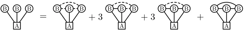
Figure 3: An example of interpreting a drawing of a decorated graph with some unspecified adjacencies.

Lemma 6. Let k ∈ N_{, let a1, . . . , ak be positive real numbers summing to one, and let} d1, . . . , dk be distinct reals between zero and one. If W is a partitioned graphon with k

parts formed by vertices of degree di and measure ai each, then any decorated constraint

can be expressed as a single ordinary constraint, i.e. W satisfies the decorated constraint if and only if it satisfies the ordinary constraint.

By Lemma 6, we can equivalently work with (formally stronger) decorated constraints instead of ordinary constraints.

It is useful to fix some notation for visualizing decorated constraints. We write the decorated constrains as expressions involving decorated graphs where the roots are depicted by squares and non-root vertices by circles, and each vertex is labeled with the name of the respective part of a graphon. The solid lines connecting vertices correspond to the edges and dashed lines to the non-edges. No connection between two vertices means that both edge or non-edge are allowed between the vertices, i.e. the picture should be interpreted as the sum of two graphs, one with an edge and with a non-edge. If more than a single pair of vertices is not joined, the picture should be interpreted as the multiple sum over all non-joined pairs of vertices, which can lead to a sum containing several isomorphic copies of the same decorated graph. An example is given in Figure 3. To avoid possible ambiguity, the drawings of the subgraph induced by the roots are identical for all decorated graphs in each constraint, which makes clear which roots correspond to each other.

first constraint on the last line in Figure 9, where a coefficient to account for isomorphisms of the two graphs appearing in the constraint would have to be included.

We finish this section with the following lemma, which is an easy corollary of Lemma 6. In essence, it says that if a graphon W0 can be finitely forced in its own right, then it can

be forced on a single part of a partitioned graphon W without affecting the structure of the other parts.

Lemma 7. LetW0 be a finitely forcible graphon, let a1, . . . , ak be positive reals summing to

one and let d1, . . . , dk be distinct reals between zero and one. Then there exists a finite setC

of decorated constraints such that a partitioned graphon W with k parts formed by vertices of degree di and measure ai each satisfies C if and only if the subgraphon of W induced by

the m-th part is weakly isomorphic to W0. In other words, if the m-th part is denoted Am,

then W satisfies C if and only if there exist measure preserving mapsϕ : [0, am]→Am and ϕ0 : [0,1]→[0,1] such that W(ϕ(xam), ϕ(yam)) =W0(ϕ0(x), ϕ0(y)) for almost every pair

(x, y)∈[0,1]2_.

Proof. LetH1, . . . , Hℓ and d1, . . . , dℓ be the subgraphs and their densities such that W0 is

the unique graphon (up to weak isomorphism) with these densities. The set C is formed by

ℓ decorated constraints: the left side of thei-th constraint contains Hi with all its vertices

labelled byAm and the right side is equal todi divided by the number of automorphisms of Hi. If the subgraphon ofW induced by Am is weakly isomorphic toW0, then clearly these

constraints are satisfied. On the other hand, since W0 is forced by setting the densities of Hi todi for every i∈[ℓ], the converse is true as well.

6

Finite forcibility of the ˇ

Svejk graphon

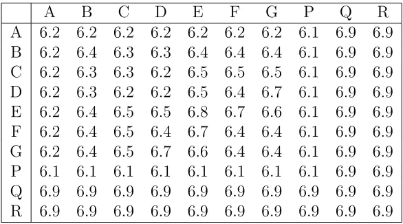
Our final and longest section is devoted to proving that the ˇSvejk graphon is finitely forcible. We will prove this by exhibiting a finite set of constraints that the ˇSvejk graphon satisfies and showing that the ˇSvejk graphon is the only graphon up to weak isomorphism that satisfies this set of constraints. By Lemma 5, there exists a finite set of constraints such that any graphon that satisfies them is a partitioned graphon with ten parts of the sizes as in the ˇSvejk graphon and degrees of vertices in these parts as in Table 3. Hence, we can work with decorated constraints with vertices labeled by the parts A, . . . , G,P, Q

and R (see Lemma 6). We will use decorated constraints to enforce the structure of the graphon between pairs of its parts, one pair after another, often building on the structure enforced by earlier constraints. Table 4 gives references to subsections where the structure between the particular pairs of parts is forced.

Fix a graphon W0 that satisfies all the constraints presented in this section. In

particu-lar, W0 satisfies the constraints given by Lemma 5 and it is a partitioned graphon with ten

parts of the sizes as in the ˇSvejk graphon and degrees of vertices in these parts as in Table 3. These ten parts of W0 will be denoted by A0, . . . , G0, P0, Q0 and R0 in correspondence

with the parts of the ˇSvejk graphon. We will show that W0 is weakly isomorphic to the

ˇ

A B C D E F G P Q R A 6.2 6.2 6.2 6.2 6.2 6.2 6.2 6.1 6.9 6.9 B 6.2 6.4 6.3 6.3 6.4 6.4 6.4 6.1 6.9 6.9 C 6.2 6.3 6.3 6.2 6.5 6.5 6.5 6.1 6.9 6.9 D 6.2 6.3 6.2 6.2 6.5 6.4 6.7 6.1 6.9 6.9 E 6.2 6.4 6.5 6.5 6.8 6.7 6.6 6.1 6.9 6.9 F 6.2 6.4 6.5 6.4 6.7 6.4 6.4 6.1 6.9 6.9 G 6.2 6.4 6.5 6.7 6.6 6.4 6.4 6.1 6.9 6.9 P 6.1 6.1 6.1 6.1 6.1 6.1 6.1 6.1 6.9 6.9 Q 6.9 6.9 6.9 6.9 6.9 6.9 6.9 6.9 6.9 6.9 R 6.9 6.9 6.9 6.9 6.9 6.9 6.9 6.9 6.9 6.9

Table 4: The subsections of Section 6 where the structure of the ˇSvejk graphon between the corresponding pairs of parts is forced.

ξ and ξx, in a way specific to individual subsections. The meaning will clearly be defined

in the corresponding subsection, so no confusion could appear.

6.1

Coordinate system

The half-graphon W△, i.e. the zero-one graphon defined by W△(x, y) = 1 iff x+y ≥ 1,

is finitely forcible [13], also see [31]. By Lemma 7, there exists a finite set of decorated constraints such that W0 satisfies these constraints if and only if the subgraphon induced

by the part P0 is weakly isomorphic to the half-graphon W△. We insist that W0 satisfies

these constraints.

Let X ∈ {A, . . . , G, P}. We use the symbol X0 to refer to the corresponding element

of {A0, . . . , G0, P0}. By the Monotone Reordering Theorem (see [29, Proposition A.19] for

more details), there exist measure preserving mapsϕX :X0 →[0,|X0|) and non-decreasing

functions fX : [0,|X0|)→[0,1), such that

fX(ϕX(x)) = 13 Z

P0

W0(x, z) dz

for almost every x∈X0. Since we already know that the subgraphon ofW0 induced by P

is weakly isomorphic to W△, we must have W0(x, y) = 1 for almost every pair (x, y)∈P02

with fP(ϕP(x)) +fP(ϕP(y)) ≥ 1, W0(x, y) = 0 for almost every pair (x, y) ∈ P02 with fP(ϕP(x)) +fP(ϕP(y))<1, andfP(z) = 13z for almost every z ∈[0,1/13).

Set gX(x) =fX(ϕX(x)) for x ∈ X0 and X ∈ {A, . . . , G, P}. For completeness, let gQ

and gR be any measurable maps from Q0 and R0 to Q ∼= [0,4) and R ∼= [0,1) such that

X of the graphon W13. The maps gA, . . . , gG, gP, gQ and gR constitute a mapg from the

vertices of W0 to the vertices of W13 and so to those of WS.

We will argue that the map g as a map from the vertices W0 to the vertices of WS is

measure preserving and we will show that W0(x, y) = WS(g(x), g(y)) for almost every pair

(x, y)∈ [0,1]2_{. This will prove that the graphons W}

0 and WS are weakly isomorphic. So

far, we have established that W0(p, p′) =WS(g(p), g(p′)) for almost every pair (p, p′)∈P02

and that the mapg is measure preserving when restricted to P0∪Q0∪R0.

P X

P X

= 0

P Y

=

P P

P Z

= 1

−

P P

Figure 4: Decorated constraints used in Subsection 6.1 where X ∈ {A, B, C, D, E, F, G},

Y ∈ {E, F, G}and Z ∈ {A, B, C, D}.

Let us consider the decorated constraints depicted in Figure 4. Let NX(x) = {y ∈ X0 | W0(x, y) = 1} for x ∈ P0 and X ∈ {A, . . . , G}. The first constraint implies that

the graphon W0 is zero-one valued almost everywhere on P0 ×(A0 ∪ · · · ∪G0) and that NX(x)\NX(x′) orNX(x′)\NX(x) has measure zero for almost every pair (x, x′)∈P02 and

for every X ∈ {A, . . . , G}. The second constraint in Figure 4 implies for Y ∈ {E, F, G}

that the measure of NY(x) is gP(x) for almost every x ∈ P0. Hence, it must hold that fY(y) = 13y for y ∈ [0,1/13) and W0(x, y) = 1 for almost every (x, y) ∈ P0 ×Y0 with gP(x) +gY(y)≥1. Similarly, the third constraint in Figure 4 implies forZ ∈ {A, B, C, D}

that the measure of NZ(x) is 1−gP(x) for almost every x ∈ P0. Consequently, it holds

that fZ(y) = 13y fory∈[0,1/13) and W0(x, y) = 1 for almost every (x, y)∈P0×Z0 with gP(x)≥gZ(x). We conclude thatg is a measure preserving map on the whole domain and W0(x, y) =WS(g(x), g(y)) for almost every pair (x, y)∈P0×(Q0∪R0).

The values of the functions gA, . . . , gG can be understood to be the coordinates of the

vertices in A0, . . . , G0, respectively, and the coordinate of a vertex x∈A0∪ · · · ∪G0 is

gX(x) = 13 Z

P0

W0(x, z) dz

for X ∈ {A, . . . , G}. This integral is easily expressible as a decorated density expression since it is just the relative edge density (degree) of x to P0. This view allows us to

speak about segments and subsegments of the parts A0, . . . , G0. The k-th segment of X0, X ∈ {A, . . . , G}, is formed by those x ∈ X0 such that [gX(x)]1 = k. Analogously, the

values [gX(x)]2 determine the subsegments.

6.2

Segmenting

We now force that the parts A0, . . . , G0 of W0 are split into segments as in WS. We also

force the structure to recognize the first segment through the clique inside D2

the “successor” relation on the segments through the structure insideC0×D0. All three of

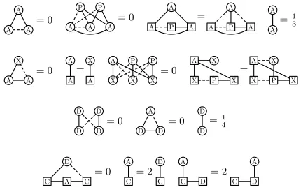
these aims will be achieved by the decorated constraints given in Figure 5; the arguments follows those given in [17, 18].

A A A

= 0

A A A P P

= 0

A P A A P A

A A

=

A A

=

A A X

= 0

A A

A X

=

X X X A P P

= 0

X P X X P X

X X

A A

=

D D D D

= 0

D D A

= 0

D D

=

C A C D

= 0

C A

C D

= 2

C D C D

A A

= 2

Figure 5: Decorated constraints used in Subsection 6.2 where X ∈ {B, C, D, E, F, G}.

The four constraints on the first line in Figure 5 force the structure on A2

0. The first

constraint implies that there exists a set J of disjoint measurable subsets of A0 such that

for almost every x ∈ A0, there exists J ∈ J such that W0(x, y) = 1 for almost every x, y ∈ J and W0(x, y) = 0 for almost every x ∈ J and y 6∈ J. Hence, W0(x, y) = 1 for

almost every (x, y)∈S

J∈J J2 and W0(x, y) = 0 for almost every (x, y)∈A20 \ S

J∈J J2.

We claim that the second constraint together with the structure on A0×P0 yields that

for every set J ∈ J there exists an open intervalJ′ _{⊆[0,1) such that J and g}−1

A (J′) differ

on a set of measure zero. Note that such an open interval J′ _{might be empty. Since we}

use an argument of this kind for the first time in this paper, we give more details. If one of the (non-null) sets J did not have the property, then a random sampling of three points x, x′_{, x}′′ _{∈ J ⊆ A}

0 with gA(x) < gA(x′) < gA(x′′) would satisfy W0(x, x′) = 0

and W0(x, x′′) = 1 with positive probability. For such three points, the probability of

sampling the additional two points fromP0 is gA(x′)−gA(x) andgA(x′′)−gA(x′) and the

triples of pointsx, x′_{, x}′′ _{such that the differencesg}

A(x′)−gA(x) andgA(x′′)−gA(x′) would

be bounded away from zero have positive measure. Let J′ _{be the set of open intervals} J′ _{⊆[0,1) such that g}−1

A (J′) and J differ on a set of measure zero for some J ∈ J. Since

The third constraint implies that if x, x′ _∈g−1

A (J′) for some J′ ∈ J′, then the measure

of the interval J′_{, assuming it is non-empty, and the measure of the interval (supJ}′_{,1) are}

the same. Again, we provide a detailed justification since we use an argument of this kind for the first time. Almost every choice of the three roots x∈A0,x′ ∈P0 and x′′ ∈A0 (the

order follows that in the figure) satisfies that gA(x) < gP (x′) < gA(x′′) (because of the

non-edge between xand x′ _{and the edge between x}′ _{and x}′′_{) and that there exists J}′ _{∈ J}′

such that x, x′′ _{∈ g}−1

A (J′) (because of the edge between x and x′′). The left side is then

equal to the measure of g_A−1(J′_{), which is the measure of J}′_{. The right side is equal to the}

measure of those z ∈A0 such that z 6∈g_A−1(J′) and gA(z)> gP (x′). Hence, the right side

is equal to 1−supJ′_{. Since this holds for almost every triple x, x}′ _{and x}′′_{, we conclude}

that the measure of each non-empty interval J′ _{∈ J}′ _{is 1−supJ}′_{. Consequently, each}

non-empty interval J′ _{must be of the form (1−2α,1−α) for some α ∈ [0,1). Since the}

intervals ofJ′ _{are disjoint, there can only be a finite number of intervals to the left of each}

interval ofJ′_{. This implies that the set J}′ _{is countable.}

Finally, the last constraint on the first line yields that

Z

A2 0

W(x, y) dxdy= X

J′_∈J′

(supJ′−infJ′)2 = 1 3 .

However, this equality can hold only if the intervals contained inJ′_{are exactly the intervals}

1−21−k_,1−2−k

, k ∈ N_{. We conclude that W0(x, y) and WS(g(x), g(y)) are equal for}

almost every pair (x, y)∈A2 0.

We now analyze the four constraints on the second line in Figure 5. FixX ∈ {B, . . . , G}. The first constraint implies that for everyJ ∈ J, there existsZJ ⊆X0such thatW0(x, y) =

1 for almost every (x, y)∈J×ZJ and W0(x, y) = 0 for almost every (x, y)∈J×(X0\ZJ).

The second constraint yields that the measure of ZJ is the same as the measure ofJ. The

third constraint implies that there exists an open interval Z′

J such that ZJ and gX−1(ZJ′)

differ on a set of measure zero. Finally, the last constraint on the second line yields that each of the intervals Z′

J is of the form (1−2α,1−α) for some α∈[0,1). Since the length

of Z′

J is the same as the measure of J, we conclude that if J = g−1A ((1−21−k,1−2−k)),

then Z′

J = (1−21−k,1−2−k). Hence, W0(x, y) and WS(g(x), g(y)) are equal for almost

every pair (x, y)∈A0×X0, X ∈ {B, . . . , G}.

Let us turn our attention to the three constraints on the third line in Figure 5. The first constraint implies that there exists a subset ZD of D0 such that W0(x, y) = 1 for

almost every (x, y)∈Z2

D and W0(x, y) = 0 for almost every (x, y)∈D02\ZD2. The second

constraint yields that ZD is a subset of ZJ for some J ∈ J. Finally, the third constraint

says that the square of the measure of ZD is 1/4, i.e. the measure of ZD is 1/2. However,

this is only possible if ZD and gD−1((0,1/2)) differ on a set of measure zero. We conclude

that W0(x, y) andWS(g(x), g(y)) are equal for almost every pair (x, y)∈D20.

It remains to analyze the three constraints on the last line in Figure 5. The first constraint yields that for every k ∈ N_{, there exists Zk ⊆ D0 such that W(x, y) = 1 for}

almost every (x, y) ∈ g_C−1((1 −21−k_,1−2−k_))×Z

k and W(x, y) = 0 for almost every

(x, y)∈g_C−1((1−21−k_,1−2−k_))×(D

of Zk is 2−k−1, and the third constraint that Zk is a subset of gD−1((1−2−k,1−2−k−1))

except for a set of measure zero. Hence, Zk and gD−1((1−2−k,1−2−k−1)) differ on a set of

measure zero, and we can conclude that W0(x, y) andWS(g(x), g(y)) are equal for almost

every pair (x, y)∈C0×D0.

6.3

Tower function

In this subsection, we will force a representation of the tower inside B0 ×D0. This is

achieved using the constraints depicted in Figure 6. Before analyzing these constraints, we give an analytic observation based on [31, proof of Lemma 3.3].

Lemma 8. Let F : [0,1)2 _{→[0,1) be a measurable function. If} Z

[0,1)

F(x, z)F(y, z)dz =ξ

for almost every (x, y)∈[0,1)2_{, then}

Z

[0,1)

F(x, z)2 dz =ξ

for almost every x∈[0,1).

The constraint on the first line in Figure 6 yields that



 Z

C0

W0(x, z)W0(y, z) dz   2 =   Z C0

W0(x′, z)W0(x′′, z) dz     Z C0

W0(y′, z)W0(y′′, z) dz 



for almost every x, x′_{, x}′′ _{∈ C}

0 and y, y′, y′′ ∈ A0 all in the same segment (this is implied

by the presence of the edges between the roots). By Lemma 8, we get that



 Z

C0

W0(x, z)W0(y, z) dz   2 =   Z C0

W0(x′, z)2 dz     Z C0

W0(y′, z)2 dz 



for almost every x, x′ _∈C

0 and y, y′ ∈A0 such that [gC(x)]1 = [gA(y)]1. Since the equality

holds for almost every x, x′ _∈C

0 and y, y′ ∈A0, it actually holds that 

 Z

C0

W0(x, z)W0(y, z) dz   2 =   Z C0

W0(x, z)2 dz     Z C0

W0(y, z)2 dz 



for almost every x ∈ C0 and y ∈ A0 such that [gC(x)]1 = [gA(y)]1. The Cauchy-Schwarz

C C C A A A C C C C A A A C C C C A A A C C C C A A A C

×

=

×

×

=

×

=

C D A C

C C A

=

C D A C

A A C

B A B C A C

= 0

B C A C

= 0

B A B C

= 0

B A D

C D

=

C B A C D A B

C C

C B A C D A B

A A C

=

=

for almost every x ∈ C0, y ∈ A0 and z ∈ C0 with [gC(x)]1 = [gA(y)]1 = k. Hence, W0(x, z) = ξk for almost every x ∈ C0 and z ∈ C0 with [gC(x)]1 = [gC(z)]1 = k and W0(x, z) = 0 for almost every x∈C0 and z∈C0 with [gC(x)]1 6= [gC(z)]1. Along the same

line, the constraint on the second line implies that for every k ∈ N _{there exists ξ}′ k ∈ R

such that W0(x, z) = ξ′k ·W0(y, z) for almost every x ∈ B0, y ∈ A0 and z ∈ D0 with

[gB(x)]1 = [gA(y)]1 =k. Consequently, W0(x, z) =ξk′ for almost every x∈ D0 and z ∈B0

with [gD(x)]1 = [gB(z)]1 = k and W0(x, z) = 0 for almost every x ∈ D0 and z ∈B0 with

[gD(x)]1 6= [gB(z)]1.

Almost every choice of the roots in the first constraint on the third line satisfies that all the roots belong to the same segment and this segment must be the first segment because of the edge between the two roots from D0. Hence, this constraint implies that ξ1|g_C−1((0,1/2))|= 1/4, i.e. ξ1 = 1/2 as desired.

Let us now look at the second constraint. Almost every choice of the roots satisfies that if the right root from C0 is in the k-th segment, then the roots from A0 and D0 are

also in the k-th segment and the left root from C0 is in the (k−1)-th segment. Since for

every k the choice of such roots has positive probability, the constraint implies that the following holds for every k ∈N_:

ξk

g_C−1 1−2−k+1,1−2−k

2

g_A−1 1−2−k,1−2−k−1

=

g_A−1 1−2−k+1,1−2−k

2

ξk+1

g_C−1 1−2−k,1−2−k−1

.

Hence, it holds that ξk+1 = ξk2 = 2−2

k−1

. We conclude that W0(x, y) and WS(g(x), g(y))

are equal for almost every pair (x, y)∈C0×C0.

The first three constraints on the fourth line in Figure 6 yield that for every k ∈ N

either W(x, y) = 0 for almost every x ∈ B0 in the k-th segment and almost every y ∈ C0

or there exists mk such that W(x, y) = 1 for almost every x∈B0 in thek-th segment and

almost everyy∈C0 in themk-th segment and W(x, y) = 0 for almost every y∈C0 not in

the mk-th segment. The last constraint on the fourth line yields that m1 = 1.

We now show that the constraint on the fifth line implies that mk exists and mk = t(k−1) for everyk ∈N_{. For almost every choice of the roots in the constraint on the fifth}

line, if the right root from B0 belongs to the k-th segment, the left root from B0 belongs

to the (k−1)-th segment and the left root from C0 belongs to the mk−1-th segment. We

derive that this constraint implies that

2−2mk−1−1

·2−mk−1

2

= 2−mk−12_·2−mk _.

We conclude that mk = 2mk−1 and so mk = t(k − 1). Consequently, W0(x, y) and WS(g(x), g(y)) are equal for almost every pair (x, y)∈B0×C0.

The constraint on the last line in Figure 6 yields by considering a choice of the root in the k-th segment of B0 that

2−k·2−mk _=ξ′

k·2−k .

We conclude that ξ′

k = 2−mk = 2−t(k−1) =t(k)−1. Hence, W0(x, y) and WS(g(x), g(y)) are

6.4

Subsegmenting

We now force the parts of the graphon that further structure the segments, e.g., provide the structure of subsegments; these are the partsB0×(B0∪E0∪F0∪G0),F0×(D0∪F0∪G0) and G2

0. Some of the arguments are analogous to those presented earlier in Subsection 6.2. In

analogy to Subsection 6.2, the first two constraints in Figure 7 forX =B yield that there exists a setJ of disjoint open subintervals of [0,1) such thatW0(x, y) = 1 for almost every

(x, y) ∈ g−1

B (J)2 for some J ∈ J and W0(x, y) = 0 for almost all other pairs (x, y)∈ B20.

The third constraint implies that every set g_B−1(J) is a subset of g_A−1((1−2−k+1_,1−2−k₎₎

except for a set of measure zero for somek ∈N_{. Hence, each intervalJ ∈ J is a subinterval}

of (1−2−k+1,1−2−k) for some k ∈N_{. The fourth constraint withX =B yields that the}

length of each interval J is 2−k_t(k)−1_{. Finally, the first constraint on the second line can}

hold only if each interval (1−2−k+1_,1−2−k_{) containst(k) such intervals J. We conclude}

that W0(x, y) andWS(g(x), g(y)) are equal for almost every pair (x, y)∈B02.

B B X

= 0

X X X B P P

= 0

B B A

= 0

B X

B D

=

B B

=

∞

P

k=1 1 22k_t

(k) _{B P B}

X P X

= 0

Figure 7: The first set of decorated constraints used in Subsection 6.4 where X ∈ {B, E, F, G}.

ForX ∈ {E, F, G}, the first, second and fourth constraints on the first line yield that for each J ∈ J there exists an open intervalJ′ _{of the same length asJ such thatW}

0(x, y) = 1

for almost every (x, y)∈J ×J′ _{and W}

0(x, y) = 0 for almost every (x, y)∈J ×(X0\J′).

The last constraint on the second line in Figure 7 gives that the intervals J′ _{follow in the}

same order as the intervals J. Hence, W0(x, y) and WS(g(x), g(y)) are equal for almost

every pair (x, y)∈B0 ×(E0∪F0∪G0).

The set of constraints in Figure 8 is analogous to those in Figure 7. The main difference is the fourth constraint, which forces that if an interval J from the setJ′ _{corresponding to} F2

0 orG20 is a subinterval of an interval (1−2−k+1,1−2−k), then 2−kt(k)−1 2

= 2−k_{· |J|.}

Hence, the length of such an interval J must be 2−k_t(k)−2_{. The first constraint on the}

second line then forces that the interval (1 − 2−k+1_{,1 −2}−k_{) must contain t(k)}2 _such

intervals J and the order of the corresponding pairs of intervals is forced by the last constraint. We can now conclude that W0(x, y) and WS(g(x), g(y)) are equal for almost

every pair (x, y)∈F2

0 ∪G20∪(F0×D0).

Z Z X

= 0

X X X Z P P

= 0

Z X A

= 0

Z Z

B B A X

=

Z Z

=

∞

P

k=1 1 22k_t(k)2

Z P Z X P X

= 0

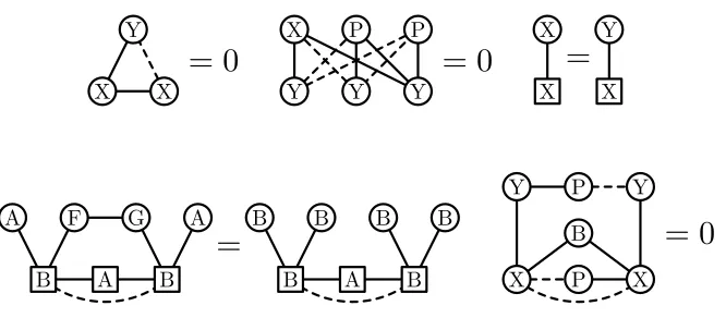
Figure 8: The second set of decorated constraints used in Subsection 6.4 where (Z, X) ∈ {(F, F),(F, D),(G, G)}.

X X Y

= 0

Y Y Y X P P

= 0

X X

X Y

=

B A B

A F G A

=

B A B

B B B B

X P X Y P Y

B

= 0

constraints on the first line force that each interval (1−2−k+1_,1−2−k_{), k ∈ N, contains}

disjoint open intervals I1, . . . , It(k)2 and J₁, . . . , J_t(k)2, each of length 2−kt(k)−2, such that W0(x, y) = 1 for almost every (x, y)∈gF−1(Ii)×g−1F (Ji) andW0(x, y) = 0 for almost every

(x, y)∈g_F−1(Ii)×(F0\g−1F (Ji)).

Fix a choice of the roots in the first constraint on the second line in Figure 9; in almost every choice of the roots, all the three roots belong to the same segment. Suppose that they belong to the k-th segment. The right side is equal to 2−kt(k)−14 for almost all choices of the roots (since the structure of B2

0 has already been forced) and the left side

is equal to 2−2k_{· 2}−k_t(k)−22 _{multiplied by the number of choices of I}

i and Ji such that Ii is contained in the subsegment of the left root and Ji in the subsegment of the right

root. Since the left side and the right side must be equal for almost all choices of the roots, we conclude that for any pair of subsegments S and S′ _{of the k-th segment there exists a}

unique index i such that Ii is contained inS and Ji inS′. The last constraint in Figure 9

enforces that for any fixed subsegment S of the k-th segment and any two subsegmentsS′

and S′′ _{such that S}′ _{precedes S}′′_{, the pairs I}

i×Ji ⊆S×S′ and Ii′ ×J_i′ ⊆S×S′′ satisfy

that the intervalIi precedes the interval Ii′. This implies thatW₀(x, y) andW_S(g(x), g(y))

are equal for almost every pair (x, y)∈F0×G0.

6.5

Binary expansions

In this section, we force the structure of the graphon inside E0×D0,E0×C0,G0×C0 and F0 ×C0. This will be achieved using the constraints depicted in Figure 10.

The first constraint on the first line in the figure causes that for almost every x∈E0,

there exists ξx such that W0(x, y) = 1 for almost every y ∈ D0 with gD(y) ≤ ξx and W0(x, y) for almost every y ∈ D0 with gD(y) > ξx. The second constraint on the line

causes that for almost every x ∈ E0, it holds that 2−[gE(x)]1ξx = 1−2−[gE(x)]1 −gE(x). It

follows that

ξx =

1−2−[gE(x)]1 _−g E(x)

2−[gE(x)]1 = 1−JgE(x)K1

for almost every x ∈ E0. We conclude that W0(x, y) and WS(g(x), g(y)) are equal for

almost every pair (x, y)∈E0×D0.

The first constraint on the second line forces that W0 is almost everywhere 0 or almost

everywhere 1 on each product of a subsegment of E0 and a segment of C0. Fix a segment SE of E0. The second constraint forces that for almost every y∈C0 the measure ofx∈SE

such that W0(x, y) = 1 is exactly half of the measure of SE. Since the measure of y∈ C0

such that W0(x, y) = 1 is 1−ξx = [gE(x)]1 for almost every x ∈ E0 because of the third

constraint on the second line, the choice of the segments and subsegments whereW0 is one

almost everywhere is unique. So, we get that W0(x, y) and WS(g(x), g(y)) are equal for

almost every pair (x, y)∈E0×C0.

The first constraint on the third line implies that for almost every x ∈ G0 there exist ξx,k,k∈ N, such thatW0(x, y) = 1 for almost everyywith [gC(y)]1 =kandJgC(y)K1 ≤ξx,k

and W0(x, y) = 0 for almost every other y ∈ C0. Consider a possible choice of the roots

E D P D

= 0

E A D

E A

E P

= 1

−

−

E B E C A C

= 0

C A C A

E E

=

E C

E D

+

= 1

C P C

G A

= 0

A B C

A P A C

G

A

B C

A P A C

=

A B C

A P A C

= 0

F A G C

= 0

F B E C

= 0

F C

=

∞

P

k=1

the leftmost root from A0 lies in the k-th segment, then the middle root from A0 is in

the t(k −1)-th segment (because of the already enforced structure of W0 on B0 ×C0 in

particular) and the rightmost root from A0 is in theℓ-th segment where ℓ ≤t(k−1). The

left side of the constraint is equal to 2−t(k−1) _{= t(k)}−1_{. The right side of the constraint}

is equal to ξx,ℓ2−ℓ. This implies that ξx,ℓ = 2ℓ/t(k) where for almost every x from the k-th segment of G0 and ℓ ≤ t(k −1). Finally, almost every choice of the roots in the

last constraint on the third line satisfies that if the leftmost root from A0 lies in the k-th

segment, then the middle root fromA0 is in thet(k−1)-th segment and the rightmost root

fromA0 is in theℓ-th segment where ℓ > t(k−1). Hence, ξx,ℓ = 0 for almost everyx from

the k-th segment ofG0 and ℓ > t(k−1). We conclude that W0(x, y) and WS(g(x), g(y))

are equal for almost every pair (x, y)∈G0×C0.

The first constraint on the fourth line implies that for almost every y ∈ C0, if the

measure of xwith W0(x, y)>0 from thek-th segment ofF0 is positive, then W0(x, y) = 1

for almost every xfrom the k-th segment ofG0. Analogously, the second constraint yields

that for almost every y ∈ C0, if the measure of x with W0(x, y) > 0 from a certain

subsegment of F0 is positive, thenW0(x, y) = 1 for almost every x from the corresponding

subsegment of G0. Consequently, W0(x, y) = 0 for almost every pair (x, y) ∈ F0 ×C0

such that WS(g(x), g(y) = 0. Since the last constraint implies that the integral of W0

over F0 ×C0 is the same as the integral of WS over F ×C, it holds that W0(x, y) and WS(g(x), g(y)) are equal for almost every pair (x, y)∈F0×C0.

6.6

Linear transformation

In this subsection, we focus on the pair G0 and E0 of the parts. The first constraint in

Figure 11 yields thatW0(x, y) = 0 for almost every (x, y)∈G0×E0 such that the segments

of [gG(x)]1 6= [gE(y)]1, i.e. the segments of x and y are different. The second constraint

implies that for almost every x ∈ G0 there exists ξx such that W0(x, y) = 1 for almost

every y ∈E0 such that [gG(x)]1 = [gE(y)]1 and JgE(y)K1 ≥ξx and W0(x, y) = 0 for almost

every y∈E0 such that [gG(x)]1 = [gE(y)]1 andJgE(y)K1 < ξx. The third constraint implies

that almost every pair of x and x′ _{from the same segment of G}

0 such thatgG(x)< gG(x′)

satisfies that ξx ≥ ξx′. In order to show that W₀(x, y) and W_S(g(x), g(y)) are equal for

almost every pair (x, y)∈G0×E0, it is enough to show that

ξx =

1

2+t([gG(x)]1 −1)

1/2

1

2−JgG(x)K1

(3)

for almost every x∈G0.

Almost every choice of the roots in the last constraint on the first line in Figure 11 satisfies that the root fromGis from the first segment. Hence, this constraint implies that almost every x ∈ G0 with [gG(x)]1 = 1 satisfies that 1−₂ξx = gG(x). Since t(0) = 1 and JgG(x)K1 = 2gG(x) for such x ∈ G0, we obtain that (3) holds for almost every x from the

first segment of G0.