Manuscript version: Author’s Accepted Manuscript
The version presented in WRAP is the author’s accepted manuscript and may differ from the published version or Version of Record.
Persistent WRAP URL:
http://wrap.warwick.ac.uk/108752
How to cite:
Please refer to published version for the most recent bibliographic citation information. If a published version is known of, the repository item page linked to above, will contain details on accessing it.
Copyright and reuse:
The Warwick Research Archive Portal (WRAP) makes this work by researchers of the University of Warwick available open access under the following conditions.
Copyright © and all moral rights to the version of the paper presented here belong to the individual author(s) and/or other copyright owners. To the extent reasonable and
practicable the material made available in WRAP has been checked for eligibility before being made available.
Copies of full items can be used for personal research or study, educational, or not-for-profit purposes without prior permission or charge. Provided that the authors, title and full
bibliographic details are credited, a hyperlink and/or URL is given for the original metadata page and the content is not changed in any way.
Publisher’s statement:
Please refer to the repository item page, publisher’s statement section, for further information.
Infinite dimensional finitely forcible graphon
∗
Roman Glebov
†Tereza Klimoˇsov´
a
‡Daniel Kr´
al’
§Abstract
Graphons are analytic objects associated with convergent sequences of dense graphs. Finitely forcible graphons, i.e., those determined by finitely many subgraph densities, are of particular interest because of their relation to various problems in extremal combinatorics and theoretical computer science. Lov´asz and Szegedy conjectured that the topological space of typical vertices of a finitely forcible graphon always has finite dimension, which would have implications on the minimum number of parts in its weak ε-regular partition. We disprove the conjecture by constructing a finitely forcible graphon with the space of typical vertices that has infinite dimension.
∗The work leading to this invention has received funding from the European Research
Coun-cil under the European Union’s Seventh Framework Programme (FP7/2007-2013)/ERC grant agreement no. 259385. A part of this work was done during a visit of the last two authors to the Institut Mittag-Leffler (Djursholm, Sweden).
†School of Computer Science and Engineering, Hebrew University, Jerusalem 9190401,
Is-rael. E-mail: [email protected]. Previous affiliations: Mathematics Institute and DIMAP, University of Warwick, Coventry CV4 7AL, UK. Department of Mathematics, ETH, 8092 Zurich, Switzerland.
‡Department of Applied Mathematics, Faculty of Mathematics and Physics, Charles
University, Malostransk´e n´am. 25, 118 00 Prague 1, Czech Republic. E-mail: [email protected]. Previous affiliation: Mathematics Institute and DIMAP, University of Warwick, Coventry CV4 7AL, UK. This author was supported by Center of Excellence — ITI, project P202/12/G061 of GA ˇCR and by the Center for Foundations of Modern Computer Science (Charles University project UNCE/SCI/004).
§Faculty of Informatics, Masaryk University, Botanick´a 68A, 602 00 Brno, Czech Republic,
1
Introduction
Analytic objects associated with convergent sequences of combinatorial objects have recently attracted significant amount of attention. This line of research was initiated by the theory of limits of dense graphs [7–9, 33], followed by limits of sparse graphs [5,15], permutations [24,25], partial orders [27] and others. Analytic methods applied to such limit objects led to results in many areas of mathematics and computer science, in particular in extremal combinatorics [1–4, 19, 21–23, 28, 29, 38–42] and property testing [26, 36].
In this paper we are concerned with limits of dense graphs and in particular with those determined by finitely many subgraph densities. This phenomenon, which is known as finite forcibility, is closely related to quasirandomness of com-binatorial objects, whose study was initiated by Chung, Graham and Wilson [12], R¨odl [43] and Thomason [45,46]. In the setting of graph limits, large dense graphs are represented by analytic objects called graphons and the just mentioned results assert that every constant graphon is finitely forcible. This result was generalized by Lov´asz and S´os [31], see also [44], who proved that every step graphon, which is a multipartite graphon with uniform densities between and within its parts, is finitely forcible.
We are interested in the structure of the space of typical vertices of finitely forcible graph limits. We consider two spaces of typical vertices, which we for-mally define in Section 2. One is the space studied in [32] and is denoted by
T(W); informally speaking, T(W) is formed by the neighbor functions (“rows” of a graphon W) with the L1-topology. The other, which is denoted by T(W),
is the space studied in [30, Chapter 13], where the L1-metric is replaced by a
finer metric. The structure of the spaceT(W) is closely related to weakε-regular partitions of W [30, 35]; in particular, if T(W) has finite Minkowski dimension, thenW has a weak ε-regular partition with a number of parts polynomial inε−1.
We note that there are graphonsW such that the minimum number of parts in a weakε-regular partition ofW is exponential in ε−2 [13]. In particular, graphons W such that the Minkowski dimension of T(W) is finite have simple structure from the regularity decomposition point of view.
Lov´asz and Szegedy [32, Conjecture 10], led by examples of finitely forcible graphons that were known at that time, conjectured that the space of typical vertices of a finitely forcible graphon always has finite dimension. We cite the conjecture verbatim.
Conjecture 1. If W is a finitely forcible graphon, then T(W) is finite dimen-sional. (We intentionally do not specify which notion of dimension is meant here—a result concerning any variant would be interesting.)
In this paper we construct a graphonW, which we call ahypercubical graphon,
Theorem 1. The hypercubical graphon W is finitely forcible and the topological
spaces T(W) and T(W) contain subspaces homeomorphic to [0,1]∞ equipped
with the product topology.
Looking at one of the motivations for studying the dimension of the spacesT(W) and T(W), we remark that every weak ε-regular partition of W has at least 2Θ(log2ε−1)
parts. We further discuss the existence of finitely forcible graphons with no weak ε-regular partition with a small number of parts in the concluding section.
The proof of Theorem 1 extends the methods from [18] and [37]. In partic-ular, Norine [37] constructed finitely forcible graphons with the space of typical vertices of arbitrarily large (but finite) Lebesgue dimension. In his construction, both T(W) and T(W) contain a subspace homeomorphic to [0,1]d. One of the
contributions of this paper is showing how the techniques from [18] and [37] can be refined to force a subspace homeomorphic to [0,1]∞, which turned out to be quite challenging. Another contribution of the paper is formalizing the methods used in [18] and [37], which are further used in the follow up papers [10, 11, 20].
We finish with giving a brief outline of the proof of Theorem 1 in informal terms. As in [18], the constructed hypercubical graphonWhas several parts (see Figure 1), which are determined by the degrees of the vertices that are contained in the parts. The partsA1, . . . , A3 serve to further partition the partsB1, . . . , B5
into infinitely many smaller parts; the partB1 is split into partsB1,d,d∈N. The
structure between the partsA1andA0 plays the role of identifying the first of the
smaller parts and the structure betweenA1andA3links consecutive smaller parts.
The part C serves to introduce coordinate systems on the parts A0, . . . , A3 and B1, . . . , B5. The structure between the partsB1 andB2 provides ad-dimensional
coordinate system on B1,d, d ∈ N, and is used to arrange that B1,d induces a
subspace homeomorphic to [0,1]d. Thed-dimensional structure of the parts B
1,d
is forced in an iterative (induction like) way, increasing the dimension by one at each step. The proof is concluded by forcing the parts B1,d to be “projections”
of the partD; in this way, we arrange that the subspace associated with the part
D is homeomorphic to [0,1]∞.
2
Definitions
In this section we present the notation that we use throughout the paper; this includes the notions from the theory of graph limits, which originated in [7–9,33].
Agraph is a pair (V, E) whereE ⊆ V2. The elements ofV are calledvertices
The density of a graph H in a graph G, which is denoted by d(H, G), is the probability that a random set of |H| distinct vertices of G induce a subgraph isomorphic to H. If |H| > |G|, we define d(H, G) to be zero. A sequence of graphs (Gi)i∈N is convergent if the sequence (d(H, Gi))i∈N converges for every
graph H. In general, we will consider sequences of graphs with their orders tending to infinity.
Convergent sequences of graphs can be associated with an analytic limit ob-ject, which we will now introduce. A graphon W is a symmetric measurable function from [0,1]2 to [0,1]. Here, symmetric stands for the property that W(x, y) = W(y, x) for every x, y ∈ [0,1]. Very imprecisely speaking, one can think of a graphon as of a continuous version of the adjacency matrix of a graph. Mimicking the terminology for graphs, we refer to a graphon W restricted to
S×T, whereS and T are two measurable subsets of [0,1], as to a subgraphon of
W induced by S×T.
We next link graphons to convergent sequences of graphs. AW-random graph
of orderk is obtained by sampling uniformly and independentlyk random points
x1, . . . , xk ∈[0,1], which are associated with the vertices, and by joining the
ver-tices corresponding to xi and xj by an edge with probability W(xi, xj). Because
of this connection, we refer to the points of [0,1] as to the vertices of W. The
densityof a graphH in a graphonW is the probability that theW-random graph
of order|H| is isomorphic to H. The definition of aW-random graph yields the following:
d(H, W) = |H|! |Aut(H)|
Z
[0,1]|H|
Y
(i,j)∈E(H)
W(xi, xj)
Y
(i,j)6∈E(H)
(1−W(xi, xj)) dλ|H| ,
where Aut(H) is the automorphism group of H. Our results do not depend on whether we work with Borel or Lebesgue measure on [0,1]d, and we have
made a choice of working with the Borel measure throughout the paper, which is denoted by λ or by λd if we wish to emphasize the dimension of the support
space. When we talk about the measure on [0,1]N, we mean the product measure
of the measures on [0,1].
One of the key results in the theory of graph limits asserts [33] that for every convergent sequence (Gi)i∈N of graphs with increasing orders, there exists
a graphonW, which is called the limit of the sequence, such that for every graph
H,
d(H, W) = lim
i→∞d(H, Gi) .
Conversely, if W is a graphon, then the sequence of W-random graphs with increasing orders converges with probability one and its limit isW.
Two graphons W1 and W2 are weakly isomorphic if d(H, W1) = d(H, W2)
opposite is true in the following sense [6]: if two graphonsW1 andW2 are weakly
isomorphic, then there exist measure preserving maps ϕ1 : [0,1] → [0,1] and ϕ2 : [0,1]→[0,1] such that W1ϕ1 =W
ϕ2
2 almost everywhere.
The degree degW x of a vertex x∈[0,1] in a graphon W is defined as
degW x= Z
[0,1]
W(x, y)dy.
Note that the degree is well-defined for almost every vertex of W. We omit the superscriptW whenever the graphon is clear from context. LetAbe a measurable non-null subset of [0,1]. The relative degree degWA x of a vertex x ∈ [0,1] with respect A is defined as
degWA x= R
AW(x, y)dy
λ(A) .
Fix a graphon W, x, x0 ∈ [0,1] and a measurable set Y ⊆ [0,1]. The set
NY(x) is the set of y ∈Y such that W(x, y)>0 and
NY(x\x0) = {y ∈Y |W(x, y)>0 andW(x0, y)<1}.
Informally speaking, NY(x\x0) contains y ∈ Y such that a vertex associated
with y can be a neighbor of a vertex associated with x and a non-neighbor of a vertex associated with x0 in a W-random graph. We note that, assuming that
Y is measurable, NY(x) and NY(x\x0) are measurable for almost every x and
almost every pair x and x0, respectively.
As mentioned in the Introduction, the structure and the complexity of a graphon can be studied by analyzing a topological space associated with its typ-ical vertices [34]. We now give the formal definitions of the two types of such spaces that we mentioned in the Introduction. For a graphon W and x∈ [0,1], define a function fxW : [0,1]→[0,1] to be
fxW(y) :=W(x, y).
Since the functionfW
x belongs toL1([0,1]) for almost everyx∈[0,1], the graphon
W naturally defines a probability measure µ on L1([0,1]). The space T(W) is formed by the support of the measure µ equipped with the topology inherited from L1([0,1]). A vertex x of the graphon W is called typical if fW
x ∈ T(W).
Another topological space, which is denoted byT(W), can be defined using the notion ofsimilarity distance. If f and g are two functions fromL1([0,1]), define
dW(f, g) :=
Z
[0,1]
Z
[0,1]
W(x, y)(f(y)−g(y))dy
dx.
Note that the similarity distancedW depends on the graphonW. The spaceT(W)
the topology given by the metricdW. The structure of the spaceT(W) is related
to weak regularity partitions ofW; in particular, if the Minkowski dimension of
T(W) is d, then W has a weak ε-regular partition with O(ε−d) parts. We refer
the reader to [30, Chapter 13] for further details.
2.1
Finite forcibility
A graphon W is finitely forcible if there exist graphs H1, . . . , Hk such that every
graphonW0satisfyingd(Hi, W) =d(Hi, W0) for everyi∈[k] is weakly isomorphic
toW. For example, the result of Diaconis, Holmes, and Janson [14] is equivalent to the statement that the half-graphonW4(x, y), which is defined asW4(x, y) = 1, if x+y ≥ 1, and W4 = 0, otherwise, is finitely forcible. We refer the reader to [32] for further examples of finitely forcible graphons and to Section 6 for the discussion of some further results on finitely forcible graphons.
Following the framework from [18], when proving that a graphon is finitely forcible, we give a set of constraints that uniquely determines W rather than listing the finitely many graphs and their densities that uniquely determine W.
A constraint is an equality between two density expressions, where a density
expressionis a formal real polynomial combination of graphs, i.e., a real number
or a graphHare density expressions, and ifD1andD2 are two density expression,
then the sum D1 +D2 and the product D1·D2 are also density expressions. A
graphon W satisfies a constraint D1 = D2 if both D1 and D2 are equal when
evaluated with eachH substituted withd(H, W). As it was observed in [18], if a graphon W is a unique (up to weak isomorphism) graphon that satisfies a finite setC of constraints, then the graphon W is finitely forcible. In particular, W is the unique (up to weak isomorphism) graphon with densities of graphs appearing inC equal to their densities in W.
In [18], it was also observed that a more general form of constraints, called
rooted constraints, can be used to prove that a graphon is finitely forcible. A
graph is rooted if it hasm distinguished vertices labeled with numbers 1, . . . , m; these vertices are referred to asrootswhile the other vertices arenon-roots. Two rooted graphs arecompatible if the subgraphs induced by their roots are isomor-phic through an isomorphism mapping the roots with the same label to each other. Similarly, two rooted graphs are isomorphic if there exists an isomorphism mapping thei-th root of one of them to the i-th root of the other; in particular, if two rooted graphs are isomorphic, then they are compatible.
A rooted density expression is a formal real polynomial combination of
com-patible rooted graphs. We next describe how constraints formed by rooted ex-pressions are interpreted. Consider a graphon W and a rooted graph H with
m roots, and let H0 be the graph induced by the m roots of H. We define the
auxiliary function cH : [0,1]m → [0,1]; the value of cH(x1, . . . , xm) is equal to
cH(x1, . . . , xm) = (|H|−m)!
|Aut(H)|
R
(xm+1,...,x|H|)∈[0,1]|H|−m Q
(i,j)∈E(H)
W(xi, xj) Q (i,j)6∈E(H)
(1−W(xi, xj)) dλ|H|−m,
where Aut(H) is the group of automorphisms ofH that preserves the roots, and the vertices of H are numbered in a way that the first m vertices are the roots (in the order that they have).
LetD=D0 be a constraint such thatDandD0 are compatible rooted density expressions with graphs containing m roots. For every graph H appearing in
D and D0, substitute the function cH; both D and D0 can now be viewed as
functions cD and c0D from [0,1]m to [0,1]. We say that the graphon W satisfies
the constraint D = D0 if the functions cD and c0D are equal almost everywhere.
We comment that, on several occasions, we consider constraints containing a fraction of two rooted density expressions D/D0. A constraint containing such fractions should be understood as saying that both sides are multiplied by the denominators of all the fractions, e.g., D1/D01 =D2/D20 should be understood as D1·D02 =D2·D10. One of the results in [18] asserts that for every two compatible
rooted density expressions D and D0, there exist density expressions C and C0
such that a graphonW satisfies D=D0 if and only if it satisfies C=C0.
A graphon W is partitioned if there exist k ∈ N, positive reals a1, . . . , ak
summing to one and distinct reals d1, . . . , dk between 0 and 1 such that the set
of vertices ofW with degreedi has measureai; we writeAi for the set of vertices
of degreedi for i∈[k] and refer toAi as to apart of the graphon W.
A graph H is decorated if its vertices are labeled with parts A1, . . . , Ak. The
density of a decorated graph H in a graphon W is the probability that the W -random graph is the graph H conditioned on the event that all sampled vertices are in the parts corresponding to their labels. For example, ifH is an edge with its two vertices labeled with partsA1 and A2, then the density of H inW is the
density of edges between the partsA1 and A2, i.e.,
d(H, W) = 1
λ(A1)λ(A2) Z
A1
Z
A2
W(x, y) dxdy .
Similarly as in the case of non-decorated graphs, we can define rooted decorated graphs, rooted decorated density expressions and form constraints using such expressions. A constraint that uses (rooted or non-rooted) decorated graphs is referred to asdecorated. One of the results from [18], which we state as Lemma 3, asserts that for every decorated constraint, there exists an equivalent ordinary constraint.
The structural properties of a graphon W that satisfies a given set of con-straints can be analyzed in several different ways. The concon-straints of the form
proper-ties of such graphons in an analytic way, which is the way that we will generally use in our exposition.
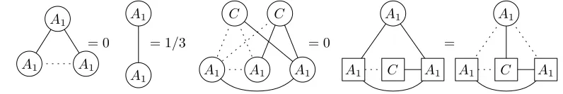
We next introduce the convention for depicting decorated constraints used throughout the paper; an example of the use of this convention can be found in Figure 4. The roots of decorated graphs will be depicted by squares and non-root vertices by circles; all vertices will be labeled by the names of the correspond-ing parts of a graphon. The full lines connectcorrespond-ing vertices correspond to edges and dashed lines to non-edges. No connection between a pair of vertices rep-resents that both edge or non-edge are allowed between the vertices, i.e., the corresponding density expression should be understood as the sum of the expres-sions containing the graph with and without such the edge (unless the edge is missing between two roots). For example, if three pairs of vertices are missing a connection, the density expression is the sum of all eight graphs that can be obtained by including or not including the edge between the three pairs. If the edge is missing between two roots, then the density constraint is required to hold both when the edge is included between the pair of root vertices in all graphs and when it is included in no graph. To avoid any possible ambiguity with interpreta-tions of the drawings of rooted constraints, the posiinterpreta-tions of the roots of all graphs appearing in a rooted decorated density constraint will always be identical (see Figure 15 for an example).
We conclude this section by explicitly stating three lemmas that were proven in [18] and that we use further. The first lemma guarantees the existence of a set of constraints that force a graphon satisfying these constraints to be a partitioned graphon with a given partition and given degrees.
Lemma 2. Letk ∈N, a1, . . . , ak be positive real numbers summing to one and let
d1, . . ., dk be distinct reals between0and 1. There exists a finite set of constraints
C such that a graphon W satisfies C if and only if W is a partitioned graphon
withk parts such that the i-th part has measure ai and its vertices have degree di.
The following lemma says that decorated constraints have the same expressing power as non-decorated constraints.
Lemma 3. Let k ∈ N, let a1, . . . , ak be positive real numbers summing to one,
and letd1, . . . , dk be distinct reals between zero and one. Further, letD1 andD2 be
two compatible rooted decorated density expressions with decorations A1, . . . , Ak.
There exist an ordinary density expression D, i.e., D has no roots and no
deco-rations, such that every partitioned graphonW withk parts formed by vertices of
degree di and measure ai each satisfies D1 =D2 if and only if it satisfies D= 0.
con-part A
0 A1 A2 A3 B1 B2 B3 B4 B5 C D E1 E2 F
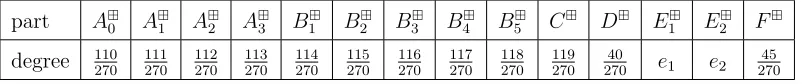
[image:10.612.93.494.109.151.2]degree 110270 111270 112270 113270 114270 115270 270116 117270 118270 119270 27040 e1 e2 27045
Table 1: The degrees of the vertices in the parts of the graphonW.
The last lemma states that there exists a finite set of constraints guaranteeing that a partitioned graphon is constant between a specific pair of its parts.
Lemma 4. For all k∈N, positive reals a1, . . . , ak summing to one, distinct reals
d1, . . . , dk between zero and one, `, `0 ≤ k, l =6 l0, and p ∈ [0,1], there exists a
finite set of constraints C such that every partitioned graphon W with k parts
A1, . . . , Ak such that the measure of Ai is ai and all vertices of Ai have degrees
di satisfies C if and only if W(x, y) =p for almost every x∈A` and y∈A`0.
3
The hypercubical graphon
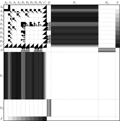
In this section, we define the graphon from Theorem 1; the graphon is denoted byW and referred to as thehypercubical graphon. For convenience, we provide
a sketch of the structure of the graphonW in Figure 1.
The hypercubical graphon W is a partitioned graphon with 14 parts, which
are denoted byA0, . . . , A3, B1, . . . , B5, C, D, E1, E2, F. Each part has mea-sure 1/27 except for the parts E
1 and E2 that have measure 11/27 and 4/27,
respectively. The degrees of the vertices in the parts are listed in Table 1. We will not compute the exact values e1 and e2 of the degrees of vertices in E1
and E
2 , respectively; however, the definition of the graphon will imply that e1 ∈(4.5/27,10/27) ande2 <1/27. In particular, vertices in different parts have
different degrees. The high level overview of the roles of individual parts of the hypercubical graphon can be found at the end of Section 1.
We describe the graphon W as a collection of functions WX×Y on products of the partsX and Y. To simplify our exposition, we define these as functions from [0,1]2 to [0,1], assuming that we have a fixed measurable bijectionη
X from
each part X to [0,1] such that λ η−1
X (S)
= λ(S)λ(X) for every measurable
set S ⊆ [0,1]. So, it holds W(x, y) = WX×Y(ηX(x), ηY(y)) for x ∈ X and
y ∈ Y, i.e., the graphon W
consists of appropriately scaled functions WX×Y.
Note that, unlike graphons, the functions WX×Y need not to be symmetric if
X 6=Y; however, these functions satisfy WX×Y(x, y) =WY×X(y, x).
We now introduce additional notation used in the definition of the graphonW
and in the proof. Forx∈[0,1), lethxibe suchk∈Nthatx∈[1−2−k+1,1−2−k) and let xb = (x− (1−2−k+1))·2k. Informally speaking, we imagine [0,1] as
A0A1A2A3B1B2B3B4B5 C D E1 E2 F
A0
A1
A2
A3
B1
B2
B3
B4
B5
C D
E1
E2
[image:11.612.94.490.167.566.2]F
Figure 1: The hypercubical graphon. The origin of the coordinate system is in the top left corner; the values of the graphon are visualized using different shades of gray (with white being zero and black being one). The graphon between the parts
X and Y, X ∈ {B
1, D} and Y ∈ {B1, B2, B4, B5}, is drawn in an imprecise
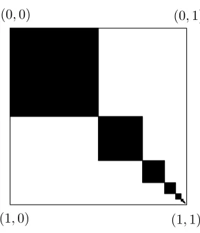
this interval. Observe thatx= 1−21−hxi+x/b 2hxi for everyx∈[0,1). Using this notation, we define the diagonal checker function κ : [0,1]2 → [0,1] as follows
(see Figure 2):
κ(x, y) =
1 if hxi=hyi
0 otherwise.
We are now ready to start with defining the structure between different parts of the graphonW.
WA0×A1
(x, y) =
1 for (x, y)∈[0,1]×[0,1/2], and
0 otherwise.
WA1×A1
= W
A1×A2
= W
A1×B1
= W
A1×B2
= W
A1×B3
= W
A1×B4
= W
A1×B5
=WA2×A3
=W
A2×B2
=κ.
ForX ∈ {A0, . . . , A3, B2, . . . , B5, C}, let:
WC×X(x, y) =
1 for x+y≥1, and
0 otherwise.
The rest of the definition of the graphon W depends on a collection of mea-sure preserving functions, which we call a recipe. A recipe R is a set of mea-sure preserving maps rn for n ∈ N∗ such that rn : [0,1] → [0,1]n. Recall that
N∗ = N∪ {∞} and so we understand [0,1]∞ to be [0,1]N. An example of a
recipe is a collection of maps that “zip” the standard binary representations of
xi, i.e., the digits of rn(x) on the positions congruent to i modulo n are
de-termined by the digits of xi, i ∈ [n], and the digits of r∞(x) on the positions
(0,0) (0,1)
[image:12.612.218.363.536.705.2](1,0) (1,1)
congruent to 2i−1 modulo 2i are determined by the digits of xi, i ∈N. Observe
that R={rn|n ∈N∗} is a recipe if and only if
λ({x|∀i∈[n] (rn(x))i ≤zi}) = n
Y
i=1
zi for every (z1, . . . zn)∈[0,1]n (1)
for every n∈N and
λ({x|∀ i∈[k] (r∞(x))i ≤zi}) = k
Y
i=1
zi for every (z1, . . . zk)∈[0,1]k (2)
for everyk ∈N, where (x)i is the i-th coordinate of x∈[0,1]n, n∈N∗. A recipe
isbijective if all the mapsrn,n ∈N∗, are bijective.
For the rest of the definition of the graphon W, we fix a bijective recipe R. It can be shown that the definition of W does not depend on this choice in the sense that the graphons defined for different choices ofR are weakly isomorphic (this statement stays true even ifR is a recipe that is not bijective).
WA1×A3
(x, y) =
1 if hxi=hyi+ 1, and
0 otherwise.
WC×B1
(x, y) =
1 for (1−21−hyi) + (r
hyi(yb))1·2−hyi+x≥1, and
0 otherwise.
WB1×B1
(x, y) =
1 if (rhxi(bx))k ≤(rhyi(by))k for every k ≤min(hxi,hyi),
1 if (rhxi(bx))k ≥(rhyi(by))k for every k ≤min(hxi,hyi), and
0 otherwise.
WB1×B2
(x, y) =
1 if hxi ≥ hyi and yb≤(rhxi(bx))hyi, and
0 otherwise.
WB1×B3
(x, y) =
1 if hxi ≥ hyi, and
0 otherwise.
WB1×B4
(x, y) =
1 if hxi ≥ hyi and yb≤
hyi Q
i=1
(rhxi(xb))i, and
WB1×B5
(x, y) =
1 if hxi ≥ hyi and yb≤
hyi Q
i=1
(1−(rhxi(bx))i), and
0 otherwise.
WD×B1
(x, y) =
1 if r∞(yb)k ≤(r∞(x))k for every k ≤ hyi, and
0 otherwise.
WD×B2
(x, y) =
1 if yb≤(r∞(x))hyi, and
0 otherwise.
WD×B4
(x, y) =
1 if yb≤
hyi Q
i=1
(r∞(x))i, and
0 otherwise.
WD×B5
(x, y) =
1 if yb≤
hyi Q
i=1
(1−(r∞(x))i), and
0 otherwise.
For everyX ∈ {A0, . . . , A3, B1, . . . , B5, C}, we set:
WE1×X
(x, y) = 1−1/11
P
Y∈A
0,...,A3,B1,...,B5,C,D
degY y.
We further define
WE2×D
(x, y) = 1−1/4
P
Y∈B
1,B2,B4,B5
degY y.
WF×A1
(x, y) = 1/10 for all (x, y)∈[0,1]
2,
WF×A2
(x, y) = 2/10 for all (x, y)∈[0,1]2,
WF×A3
(x, y) = 3/10 for all (x, y)∈[0,1]2,
WF×B1
(x, y) = 4/10 for all (x, y)∈[0,1]
2,
WF×B2
(x, y) = 5/10 for all (x, y)∈[0,1]2,
WF×B3
(x, y) = 6/10 for all (x, y)∈[0,1]2,
WF×B4
(x, y) = 7/10 for all (x, y)∈[0,1]2,
WF×B5
WF×C(x, y) = 9/10 for all (x, y)∈[0,1]2.
If we have defined a function WX×Y, we set WY×X(x, y) = WX×Y(y, x). Finally, the graphon W is equal to 0 between parts X and Y such that we
have not defined a function WX×Y or WY×X. This completes the definition of the graphonW.
We now argue that e1 ∈ (4.5/27,10/27) and e2 < 1/27. Let x ∈ E1.
Since N(x) is a subset of A0 ∪ · · · ∪A3 ∪B1 ∪ · · · ∪B5 ∪C, the measure of N(x) is at most 10/27. Since it does not hold that W(x, y) = 1 for al-most all y ∈ N(x), we get that e1 < 10/27. Observe that it holds for every X ∈ {A0, . . . , A3, B2, . . . , B5, C} that degE
1 (x) > 1/2 for every x ∈ X. It follows that e1 > 4.5/27. Similarly, N(x) is a subset of D for every x ∈ E2
and it does not hold thatW(x, y) = 1 for almost all y∈N(x); this implies that
e2 <1/27.
Before proceeding further, we introduce additional notation related to split-ting parts Ai, i ∈ {1,2,3}, and Bj, j ∈ {1, . . . ,5}, into smaller pieces. For
i ∈ {1,2,3}, the set of vertices x ∈ Ai with degA 1 x = 2
−k is denoted by A
i,k
and A
i,k is called the k-th level of Ai . Similarly, Bj,k, j ∈ {1, . . . ,5}, is the set
of verticesx∈B
j such that degA 1 x= 2
−k. Note that measure of the k-th level
A
i,k is 2
−k/27; the same holds for B
j,k.
3.1
Dimension of the space of typical vertices
We finish this section with showing that both T(W) and T(W) have infinite dimension.
Proposition 5. Both T(W) and T(W) contain a subspace homeomorphic to
[0,1]∞.
Proof. Observe that every vertex contained in D is typical (both with respect
toT(W) and with respect to T(W)) and define a map h:D →[0,1]∞ as
h(x) =degW
B 2,i
x
i∈N
.
Because r∞ is a bijection, h is a bijection between D and [0,1]∞. We next show thath−1 is continuous when D is equipped with the topology of the space
T(W). To do so, we need to bound the L1-distance of the functions fW
x and
fW
x0 in terms ofh(x) and h(x0) for all x, x0 ∈D, wherefxW(y) := W(x, y).
First note that
degW
B 1,i
x= degW
B 4,i
x= Y
k∈[i]
degW
B 2,k
x and degW
B 5,i
x= Y
k∈[i]
(1−degW
B 2,k
for every x ∈ D. The value of ||fW
x −f W
x0 ||1 is the sum of the corresponding
integrals over y from B
1, B2, B4, B5 and E2. The term corresponding to the
integral overy from B
2 is equal to
∞ X
i=1
λ(B2,i) degW
B 2,i
x−degW
B 2,i x0 ,
the term corresponding to the integral over y fromB
4 is equal to
∞ X
i=1
λ(B4,i) i Y k=1 degW B 2,k x− i Y k=1 degW B 2,k x0 ,
and the term corresponding to the integral over y fromB5 is equal to
∞ X
i=1
λ(B5,i) i Y k=1
(1−degW
B 2,k
x)−
i
Y
k=1
(1−degW
B 2,k
x0) .
The term corresponding to the integral over y fromB1 is at most
∞ X
i=1
λ(B1,i)
i X k=1 degWB
2,k
x−degW
B 2,k x0 .
We next observe that i Y k=1 degW B 2,k x− i Y k=1 degW B 2,k x0 ≤ i X k=1 degWB
2,k
x−degW
B 2,k x0 and i Y k=1
(1−degW
B 2,k
x)−
i
Y
k=1
(1−degW
B 2,k
x0) ≤ i X k=1 degWB
2,k
x−degW
B 2,k x0
for everyi∈N. Since it holds thatλ(B
j,i) = 2
−i/27 forj ∈ {1,2,4,5}, we obtain
that the sum of the terms corresponding to the integrals over y from B
1, B2, B4 and B5 is at most
1 27
∞ X
i=1
2−i degW
B 2,i
x−degW
B 2,i x0 + 3 ∞ X i=1
2−i
i X k=1 degWB
2,k
x−degW
B 2,k x0 ! ,
which is equal to
7 27
∞ X
i=1
2−i degW
B 2,i
x−degW
Since the term corresponding to the integral overy fromE2 is at most the sum of the terms to the integrals over y fromB
1,B2,B4 and B5, we conclude that
||fW
x −f W
x0 ||1 ≤
14 27
∞ X
i=1
2−i degW
B 2,i
x−degW
B 2,i
x0
! .
It follows thath−1 is a continuous map from [0,1]∞toD. Since h−1 is a
contin-uous injective map from a compact space to a Haussdorf space, it follows thath
is a homeomorphism betweenD with the topology given byT(W
) and [0,1]∞.
Since the identity map fromT(W) toT(W) is injective and continuous [34], it also follows thath is a homeomorphism between D with the topology given by
T(W) and [0,1]∞.
4
Constraints
This section and the next section are devoted to the proof of the following theo-rem, which together with Proposition 5 implies Theorem 1.
Theorem 6. The hypercubical graphon W is finitely forcible.
In this section, we present the set C of the constraints that such that the graphon W is the unique graphon satisfying C. We only list the constraints contained in C and their analysis is postponed to the next section.
We present the constraints contained in the setC split into groups depending on the properties of a graphon that they force, and we informally describe these properties.
Partition constraints are the constraints given in the Lemma 2, which are
sat-isfied by partitioned graphons with the same number of parts as W and with the measures and the degrees of vertices of the parts as in W.
All the constraints that are presented in the rest are decorated constraints with vertices labelled by the parts A0, . . . , A3, B1, . . . , B5, C, D, E1, E2, F.
The zero constraints force thatW equals 0 almost everywhere on
• A0×(A0∪A2 ∪A3∪B1∪B2∪B3∪B4∪B5 ∪D∪E2∪F),
• A1×(D∪E2),
• A2×(A2∪B1∪B3∪B4∪B5∪D∪E2),
• A3×(A3∪B1∪ · · · ∪B5∪D∪E2),
= 0 X
[image:18.612.130.462.212.353.2]Y
Figure 3: Constraint forcing zero edge density.
X X
=
X X
Z
X X
Z X
E1
X Z
E1
= 1−111 P
Z∈{A0,...,A3,
B1,...,B5,C,D}
1−111 P
Z∈{A0,...,A3,
B1,...,B5,C,D}
1−111 P
Z∈{A0,...,A3,
B1,...,B5,C,D}
Figure 4: The degree unifying constraints contain the depicted constraints for all the choices of X in{A0, . . . , A3, B1, . . . , B5, C}.
• B4 ×(B4∪B5∪E2),
• B5 ×(B5∪E2),
• C×(D∪E2), • D×(D∪E1),
• E1×(E1∪E2∪F),
• E2×(E2∪F), and
• F ×F.
The constraint forcing the zero edge density between parts X and Y is depicted in Figure 3.
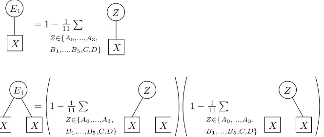
The degree unifying constraints force that the relative degree of almost every
vertex x from a part Ai, i = 0, . . . ,3, a part Bj, j = 1, . . . ,5 and the part
C with respect to the complement ofE2∪F, i.e. A0∪ · · · ∪A3∪B1∪ · · · ∪ B5∪C∪D∪E1, is equal to 1/2, and that W(x, z) is constant for almost
every such x when z ranges through the part E1. These constraints also
force that the degree of almost every vertex y from the partD is 4/27 and
W(y, z) is constant for almost every such ywhenz ranges through the part
=
Z Z
1−14 P
Z∈{B1,B2,B4,B5}
1−14 P
Z∈{B1,B2,B4,B5}
= 1−14 P
Z∈{B1,B2,B4,B5}
D
Z E2
E2
D
[image:19.612.97.484.100.323.2]D D D D D D
Figure 5: The degree unifying constraints for D.
Part A0 A1 A2 A3 B1 B2 B3 B4 B5 C
[image:19.612.136.443.289.336.2]Density 0 101 102 103 104 105 106 107 108 109
Table 2: Densities between the part F and the other parts.
The degree distinguishing constraintsforce that the graphon is constant between
the part F and each of the partsA0, . . . , A3,B1, . . . , B5,C andD, and that
this constant is equal to the value given in Table 2. The existence of finitely many such constraints follows from Lemma 4; Figure 6 contains an example of two constraints that can be used to force the graphon to be equal to 9/10 between the parts C and F.
The triangular constraints force that the structure of the subgraphon induced
by C×X is the same in W for every X ∈ A0, . . . , A3, B1, . . . , B5, C, i.e.,
that the subgraphon induced by C×X is the half-graphon. Let Hi and
di be the finitely many graphs and their densities that are satisfied by the
half-graphon only; such a finite set of graphs exists since the half-graphon is finitely forcible [14, 32]. The structure of the subgraphon induced by
C×C is forced by the constraintsHi0 =di whereHi0 is the decorated graph
obtained from Hi by labeling each vertex with C, and the structure of the
subgraphon induced by C ×X for X 6= C is forced by the constraints
F C
= 109
F F
C
F F
C = 10081
[image:19.612.219.363.636.696.2]C
C
X
C
= = 0
C C
[image:20.612.89.487.222.289.2]X X
Figure 7: The triangular constraints include the depicted constraints for all the choices of X in{A0, . . . , A3, B1, . . . , B5}.
= 0 = 1/3 A1
A1
A1
A1 A1
=
A1
A1 A1
A1 A1 A1
= 0
C C
C C
A1
A1
A1
Figure 8: The main diagonal checker constraints.
depicted in Figure 7.
The main diagonal checker constraints force the diagonal checker structure of
the subgraphon induced by A1×A1. They are depicted in Figure 8.
The complete bipartition constraints force, in particular, that the subgraphons
induced by A1×A2,A1×A3, A1×B1, . . . , A1×B5,A2×A3 and A2×B2
are unions of complete bipartite subgraphons. The constraints are given in Figure 9.
The auxiliary diagonal checker constraints determine the sizes of the sides of
complete bipartite subgraphons in A1×A2,A1×A3,A1×B1, . . . , A1×B5, A2×A3 and A2×B2. They are depicted in Figure 10.
The first level constraints force the structure of subgraphon induced byA0×A1
and they are depicted in Figure 11.
The stair constraints force the structure of subgraphon induced by B1 ×B3.
They are depicted in Figure 12.
The coordinate constraints force some properties of the structure of the
sub-graphons induced by B1×(B2 ∪B4 ∪B5) and D×(B2 ∪B4 ∪B5). They can be found in Figure 13.
The initial coordinate constraint determines the relative degrees of vertices of
B1 in a subset of B2. It is depicted in Figure 14.
The distribution constraints determine the relative degrees of vertices of B2 in
= 0 = 0
X X
X
X X
C
C Y
Y
Y
= 0 X
C
C
C = 0
Y
Y
Y
X
X Y
Y C
Figure 9: The complete bipartition constraints consist of the top two con-straint for (X, Y)∈ {(A1, A2),(A1, A3),(A1, B1), . . . ,(A1, B5),(A2, A3),(A2, B2)}
and the bottom two constraints for (X, Y) ∈ {(A1, A2), (A1, A3), (A1, B2), . . . ,
(A1, B5), (A2, A3),(A2, B2)}.
A1
=
A1 A1
Y A1
=
A2 A2
A3 A1
× −2
A1 A1
= 0 A1
−1/2 A1
[image:21.612.163.428.121.284.2]Z
Figure 10: The auxiliary diagonal checker constraints consist of the depicted constraints, whereY in the first constrains attains all values in {A2, B1, . . . , B5}
and Z in the second constraint attains all values in {A3, B2}.
A0 A1
×
A1 A1
−1/2 = 0 = 1/2 A1
A0
[image:21.612.195.392.387.525.2] [image:21.612.150.432.619.688.2]B3 A1
=
B3
B3
= 0
A2
A3
A1
A1
B1 B1
[image:22.612.174.409.147.217.2]B1
Figure 12: The stair constraints.
A1 B1 = 0
A1
C
= 0
Y Y
Y X
B3
Figure 13: The coordinate constraints consist of the depicted constraints, where
X and Y attain all values in{B1, D} and {B2, B4, B5}, respectively.
=
B1 A0
B2 A1
B1 A0
B2 A1
B1
A1
B1
A0
A1
A0
A1
C
− 1−2× A1
B1 A0
[image:22.612.160.425.532.664.2]A1
B2
D
− 1−2×
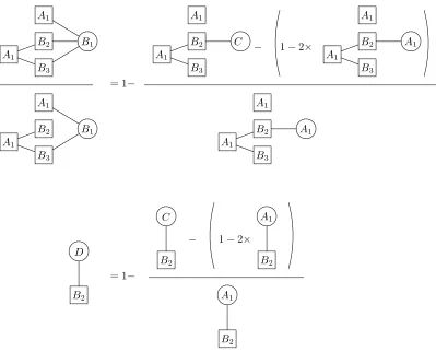
= 1− B1
A1
B2
A1
B3
B1
A1
B2
A1
B3
C A1
B2
A1
B3
A1
A1
B2
A1
B3
A1
A1
B2
A1
B3
− 1−2×
= 1−
B2
A1
B2
C
B2
[image:23.612.92.491.243.565.2]A1
A1
B1
A0
B2
A1
B1
A0
B4
=
A2 A1
= ×
A1
A0
B4
A1
A0
B2
=
B4
A3 A1
A2 A1
B4
A3 A1
X X
X
X
A2
A3 A1
A2
A3 A1
A1
B4
A1
B4
X
X
A2 A1
B2
A3 A1
A2 A1
B2
A3 A1
[image:24.612.122.461.101.322.2]X X
Figure 16: The product constraints forcing B1 ×B4 and D×B4 consist of the
depicted constraints, where X ∈ {B1, D}.
The product constraintsforce the structure of the subgraphons induced byB1×
B4, D×B4, B1×B5 and D×B5. They are depicted in Figures 16, 17.
The projection constraints force the structure of the subgraphon induced by
B1×B1. They are depicted in Figures 18 and 19.
The infinite constraints force the structure of the subgraphon iduces by D×B1
and D×B2. They are depicted in Figure 20.
This completes the list of the constraints that are contained in C
5
Proof of Theorem 6
In this section, we prove Theorem 6. In particular, we will show that the hyper-cubical graphon W is the unique (up to weak isomorphism) graphon satisfying setC of the constraints that we listed in Section 4.
Fix a bijective recipe R = {rn|n ∈ N∗}, which determines the graphon
W. Suppose that W is a graphon that satisfies all constraints contained in C. Our aim is to show that the graphons W and W are weakly isomorphic.
Since W satisfies the partition constraints, W is a partitioned graphon with parts of the same measure as those of W and the vertices in the corresponding parts having the same degree as those in W. The parts of W are denoted by
A0, . . . , A3, B1, . . . , B5, C, D, E1, E2, F in such a way that the partX corresponds
to the partX of the graphon W
A1
A0
B5
A1
A0
B2
=
A2 A1
= ×
A3 A1
A2
A3 A1
A2 A1
B2
A3 A1
A2 A1
A3 A1
A2
A3 A1
A2 A1
B2
A3 A1
A1
A1
B5
B5
B5
B5
X X
X X X
X X
[image:25.612.111.472.104.330.2]X
Figure 17: The product constraints forcing B1 ×B5 and D×B5 consist of the
depicted constraints, where X ∈ {B1, D}.
of the graphon W and A
0, . . . , F in the context of the graphon W. In the
analogy to B
1,n and B2,n, we define B1,n and B2,n to be the vertices of B1 and B2, respectively, that have relative degree 2−n with respect to A1 in W.
By the Monotone Reordering Theorem (see [30] for more details), there exist measure preserving maps ψX : X → X for X = A0, . . . , A3, B2, . . . , B5, C, E1,E2, F and non-decreasing functions fX :X →[0,1] such thatfX(ψX(x)) =
degWC xfor almost everyx∈X. Note that we have not (yet) defined the functions
ψB1 and ψD.
We now define a map gn:B1,n→[0,1]n as
gn(x) =
degWB
2,i(x)
i∈[n]
forx∈B1,n and g∞ :D→[0,1]∞ as
g∞(x) =
degWB 2,i(x)
i∈N
forx∈D. Note thatgn is well-defined almost everywhere onB1,n andg∞almost everywhere onD. We next define a map ψB1 :B1 →B
1 as
ηB−1
1
1− 1 2n−1 +
r−1
n (gn(x))
2n
.
forx∈B1,n, and we setψB1(x) to be the same arbitrary vertex of B
1 forx that
does not belong to anyB1,n, n∈N. Similarly, we define
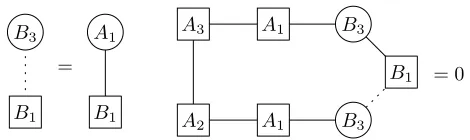
A3 A1 A1 B3 = 0 B2 B1 B1 A3
A2 A1
B2
B2
B1
B1
A1
A1 B1
A3
A2 A1
B2
B2
B1
B1
A1
A1 B1
A3
A2 A1
B2
B2
B1
B1
A1
A1 B1
A3
A2 A1
B2
B2
B1
B1
A1
A1 B1
= A3
A2
B1 B3
= B1
A1
B1
A1 A1
A3
A2
B1 B3
B1
A1
A1
A3
A2
B1 B3
A1
A1 A1
A3
A2
B1 B3
B1
A1
A1
A3
A2
B1 B3
B1 A1 A1 B4 A1 A1 B1 A1 B4 B1 A2
A2 AA11
=
A3 A1 B1
B1
B1
A2 AA11
A3 A1 B1
B1
B1 A2
A2 AA11
A3 A1 B5
B1
B1
A1
A1
A3 A1 B5
B1
[image:26.612.146.431.153.650.2]B1
A1
B1
B1
A1
B4
B1
A1
B5
B1
= +
B1
= 0
B1
A1
B2
[image:27.612.183.397.178.325.2]B2
Figure 19: The last two projection constraints.
D
B2
B1
= 0
A1
B1
A1
B4
D D
= =
B5
B1
A1
D
B1
A1
B5
B1
A1
[image:27.612.119.467.507.630.2]Let ψ be the map from [0,1] to [0,1] equal to the map ψX on the part X for
X =A0, . . ., A3, B1, . . ., B5, C, D, E1,E2,F.
In the rest of the section, we show that the graphons Wψ and W are equal almost everywhere and the mapψ is measure preserving. This would imply that the graphon W is weakly isomorphic to W. Note at this point that the maps
ψX for X 6= B1, D, which form the map ψ, are measure preserving; so we only
need to argue thatψB1 and ψD are measure preserving maps, which we will show in Subsections 5.11 and 5.12.
5.1
Zero and triangular tiles
The zero constraints guarantee that ifW is equal to zero almost everywhere on
X×Y for X, Y ∈ {A
0, . . . , A3, B1, . . . , B5, C, D, E1, E2, F}, then the graphon W is equal to zero almost everywhere onX×Y. In particular, the graphons Wψ
and W are equal almost everywhere onX×Y.
The triangular constraints that correspond to those forcing the half-graphon guarantee that the subgraphon of W induced by C×C is weakly isomorphic to the half-graphon. The choice of ψC now implies that the graphons W
ψ
and W
are equal almost everywhere onC×C. We next analyze the constraints depicted in Figure 7. Fix X ∈ {A0, . . . , A3, B1, . . . , B5}. The first constraint in Figure 7
yields that degWC (z) = degWX(z) for almost every z ∈ C. The second constraint yields thatNC(x\y) orNC(y\x) or both has measure zero for almost every pair
x, y ∈X. This implies that the graphonW has values 0 and 1 almost everywhere onX×C. The choice ofψX implies thatW andW
ψ
are equal almost everywhere
onX×C forX ∈ {A0, . . . , A3, B2, . . . , B5}. Note that we have not reached this
conclusion forX =B1 (becauseψB1 is chosen differently) but we have still shown that the graphon W is equal to 0 or to 1 almost everywhere on B1×C and that
the measure of the set containingb ∈B1 such that degCb ≤z,z ∈[0,1], is equal
tozλ(B1).
The subgraphon induced by X×C determines a preorder on the vertices of
X according to their relative degrees inC. We often use this fact in our analysis. In this context, we write x ≺X y instead of degCx < degCy for x, y ∈ X. We
also extend this notation to subsets and write Y ≺X Z for subsets Y, Z ⊆ X if
y≺X z for every y∈Y and everyz ∈Z.
5.2
Forcing the structure on
A
1×
A
1We now show that the main diagonal checker constraints, which are depicted in Figure 8, force that W and Wψ agree almost everywhere on A1×A1. Our line
of arguments follows that in [18]; we sketch the arguments and refer the reader to [18] for a more detailed analysis.
The first constraint in Figure 8 implies that ifxis a typical vertex ofA1 with
if x and x0 are two typical vertices of A1, then either NA1(x) and NA1(x
0) are
equal up to a set of measure zero or they are disjoint up to a set of measure zero. Moreover, the measure of the pairs (x, x0) such thatW(x, x0)6= 1 andNA1(x) and
NA1(x
0) are equal up to a set of measure zero is zero. LetJ
A1 be the set of disjoint non-null measurable subsets ofA1 such that each J ∈ JA1 is equal to NA1(x) up to a set of measure zero for some typical vertex x ∈A1 and each NA1(x) differs from a set contained inJA1 on a set of measure zero. Our reasoning implies that, except for a subset ofA1×A1 of measure zero,W(x, y) = 1 for (x, y)∈A1×A1
if and only ifx and y belong to the same set J ∈ JA1. Informally speaking, the graphon W on A1×A1 is a union of disjoint cliques on J ∈ JA1. Observe that since the sets contained inJA1 are non-null and disjoint, thenJA1 is countable.
The third constraint implies that for every set J ∈ JA1, there exists a set
J0 ⊆A1 differing from J on a null set such that J0 is an interval with respect to
≺A1, i.e., if x, x
0
∈J0 and x≺A1 x
00
≺A1 x
0, then x00
∈J0. Hence, we can assume without loss of generality that each J ∈ JA1 is an interval with respect to ≺A1. The fourth constraint forces that it holds for almost every two verticesx≺A1 x
0
from the sameJ ∈ JA1 that
λ(J) = λ({x00 ∈A1 | x≺A1 x
00
and x006∈J}) = λ({x00 ∈A1 | x006∈J and ∃z ∈J z ≺A1 x
00 }) .
Since the second constraint implies that P
J∈JA1
λ(J)2 =λ(A1)2/3, we obtain (see
details of the analysis in [18]) that for every J ∈ JA1, there exists k ∈ N such that J and the set
{x∈A1 | degCx∈[1−2−k−1,1−2−k]}
differ on a set of measure zero. We conclude that W agrees with Wψ almost everywhere onA1×A1.
5.3
Forcing the structure of
A
0×
A
1We now consider the first level constraints, which are depicted in Figure 11. The first constraint implies that degA
0y = 0 or degA1y= 1/2 for almost every vertex iny∈A1. In particular, W(x, y) = 0 for almost every x∈A0 and y∈A1 unless
degA1y= 1/2. The second constraint forces that the density ofW onA0×A1 is
equal to 1/2, which implies thatW(x, y) = 1 for almost everyx∈A0 and y∈A1
such that degA1y = 1/2. Therefore, W is equal to Wψ almost everywhere on
A0×A1.
5.4
Forcing remaining diagonal checker subgraphons
(A2, B2). Note that the list misses the pair (A1, B1), which is analyzed separately
afterwards.
The first constraint in Figure 9 implies that there exist a set JX formed by
disjoint non-null subsets ofX, a setJY formed by disjoint non-null subsets ofY,
and a bijectionf :JX → JY such that except for a subset of X×Y of measure
zero, it holds that W(x, y) = 1 for (x, y) ∈ X ×Y iff there exist J ∈ JX such
that x ∈ J and y ∈ f(J), and W(x, y) = 0 elsewhere on X ×Y. Informally speaking, the graphon W on X ×Y is a disjoint union of complete bipartite subgraphons betweenJ ∈ JX and f(J)∈ JY. We remark here that the set JA1 can in principle differ from the set defined in Subsection 5.2, however, we will later argue that they actually coincide (in the sense that the elements of the set differ from each other on a set of measure zero).
Analogously to Subsection 5.2, the second constraint depicted in Figure 9 implies that each set contained inJX differs from an interval with respect toX
on a set of measure zero and the third constraint implies that each set contained in JY differs from an interval with respect to Y on a set of measure zero.
Hence, we can assume without loss of generality that each set contained inJX is
an interval with respect to X and each set contained in JY is an interval with
respect toY. Finally, the fourth constraint implies that the intervals are in the
same order, i.e., if J, J0 ∈ JX satisfy that J X J0, then f(J)Y f(J0).
It remains to determine the measures of the sets contained in JX and JY.
Recall that we have shown thatW agrees withWψ almost everywhere onA1×A1.
We now split the argument depending on whetherX =A1 or X =A2 and start
with analyzing the caseX =A1. IfY 6=A3, consider the first constraint depicted
in Figure 10; this constraint implies that almost all the vertices ofX =A1 have
the same relative degree with respect to A1 as with respect to Y. Hence, almost
every x ∈ X belongs to some J ∈ JX and for every J ∈ JX, it holds that
λ(f(J)) = λ(A1) degA1x for almost every x ∈ J. Since f is a bijection and the sets contained in JY are disjoint, it follows that JX coincides with the set JA1 defined in Subsection 5.2 and λ(f(J)) =λ(J) for everyJ ∈ JX. If Y =A3, the
third constraint in Figure 10 yields that almost all the vertices of X =A1 have
either the relative degree with respect to A1 equal to 1/2 or the relative degree with respect toY double the relative degree with respect toA1; this again implies
thatJX coincides with the setJA1 defined in Subsection 5.2 andλ(f(J)) = 2λ(J) for every J ∈ JX unless λ(J) = λ(X)/2. Since the elements of JY are disjoint
intervals with respect toY and the bijectionf preserves their order, we conclude
that for every J ∈ JY, there exists k ∈N such thatJ and the set
{y ∈Y | degCy ∈[1−2−k−1,1−2−k]}
differ on a set of measure zero (this holds both if Y = A3 and if Y 6= A3). It
follows that W and Wψ agree almost everywhere on X ×Y if X = A1, i.e, W
We next finish the analysis of the case X =A2; note that Y is either A3 or B2 in this case. The second constraint depicted in Figure 10 implies that almost
all the vertices of X = A2 have the same relative degree with respect to A1 as
with respect to Y. Hence, almost every x ∈ X = A2 belongs to some J ∈ JA2 and λ(f(J)) = λ(A1) degA1x for almost every x ∈ J. Since f is a bijection, we conclude (using the already analyzed structure onA2×A1) that λ(f(J)) =λ(J)
for every J ∈ JA2. Hence, the set JA2 coincides with the set JA2 as defined in the case (X, Y) = (A1, A2), and for every J ∈ JY, there exists k ∈ N such that J and the set
{y ∈Y | degA1y ∈[1−2−k−1,1−2−k]}
differ on a set of measure zero. It follows thatW andWψ agree almost everywhere onX×Y if (X, Y) is (A2, A3) or (A2, B2).
In the previous analysis, we have omitted the case (X, Y) = (A1, B1). As in
the general caseX =A1 considered above, we derive that the top two constraints
in Figure 9 imply that there exist a set JX formed by disjoint non-null subsets
ofX that are intervals with respect to X, a setJY formed by disjoint non-null
subsets ofY, and a bijectionf :JX → JY such that except for a subset ofX×Y
of measure zero, it holds that W(x, y) = 1 for (x, y) ∈ X ×Y iff there exist
J ∈ JX such that x ∈ J and y ∈ f(J). Note that we do not make any claims
about the structure of the sets contained inJY. The first constraint in Figure 10
implies thatλ(f(J)) =λ(J) for every J ∈ JX. It follows thatJX coincides with
JA1 defined in Subsection 5.2, almost every vertex y ∈ Y belongs to J ∈ JY and the measure of y ∈Y with degA1y = 2−k is equal to 2−k. In particular, the measure of B1,k is 2−k. It follows that W and Wψ agree almost everywhere on
A1×B1.
Because each of the sets JX, X ∈ {A1, . . . , A3, B1, . . . , B5}, is the same in
all the definitions (in the sense that its elements differ from each other on a set of measure zero) that we have given in this subsection and Subsection 5.2, we can just use JX without referring to the particular place where the set was
defined. We now split each part X ∈ {A1, . . . , A3, B1, . . . , B5} into levels in the
way analogous to that the parts of W are split. For k ∈ N, the k-th level Ai,k,
i∈ {1,2}, ofAi is formed byx∈Ai such that degA1x= 2
−k, the k-th level level
A3,k of A3 is formed byx ∈A3 such that degA2x= 2
−k, and the k-th levelB i,k,
i ∈ {1, . . . ,5}, of Bi is formed by x ∈ Bj such that degA1x = 2
−k. The levels
of X coincide with sets contained JX (up to a difference on a set of measure
zero). Note that the measure of the levelAi,k or Bi,k is 2−k. Also note that this
coincides with our previous definition of B1,k.
5.5
Using levels in density expressions
A1
A2
B2
A3 A1
B1
A1
A0 A1 B1
A1
A1
B2
B2
B2
B1
B1
[image:32.612.113.467.117.197.2]B1
Figure 21: Density expressions specifying levels of vertices.
structure of W that we have already analyzed. Some examples of decorated graphs that we use are given in Figure 21. In the first decorated graph, all three vertices must belong to the same level (ignoring events with probability zero), i.e., if the root belongs to thek-th level ofA1, then the expression is equal (with
respect to W) to 2−2k, which is the product of the probabilities that a random
vertex of B1 belongs to B1,k and that a random vertex of B2 belongs toB2,k.
In the second decorated graph, if the root decorated with A2 belongs to the k-th level of A2, which is A2,k, then its neighbors must belong to A1,k and A3,k
and the remaining root toA1,k+1. In such case, the expression is equal to 2−2k−1,
which is the product of the probabilities that a random vertex ofB1 belongs to B1,k and that a random vertex of B2 belongs to B2,k+1. In the third decorated
graph, the root decorated withA1 must belong toA1,1 and the expression is equal
to 1/2, which is the probability that a random vertex ofB1 belongs toB1,1.
The final expression is more complex. Suppose that the root belongs to A1,k.
The denominator is equal to 2−2k as we have discussed earlier. The numerator
is equal to 2−2k multiplied by the density between B1,k and B2,k, i.e., the whole
expression is equal to the density ofW between the B1,k and B2,k.
5.6
Stair constraints
We now focus on the stair constraints, which are depicted in Figure 12. They are intended to force the desired structure on B1 ×B3. The first constraint in
Figure 12 determines the relative degrees of vertices ofB1 inB3, i.e., it enforces
that degB3x = 1−2−k for almost every x ∈B1,k. The second constraint forces
that the following holds for almost every vertex x ∈ B1 and every k ∈ N: if
degB
3,k+1x > 0, then degB3,kx = 1 (if degB3,kx = 0, then there exists a choice of the roots decorated with A1, A2, A3 and A1 such that the density expression is non-zero with x being the root decorated with B1). Consequently, for almost
everyx∈B1, there existsk0 ∈Nsuch thatW(x, y) = 1 for almost everyy∈B3,k,
k < k0 and W(x, y) = 0 for almost everyy∈B3,k,k > k0. However, it is possible
that degB3x= 1−2−k for almost every x ∈B
1,k only if it holds that for almost
every x ∈ B1, k0 is equal to the level of x and W(x, y) = 1 for almost every y∈B3,k0. It follows thatW agrees with W
ψ
5.7
Coordinate constraints
The coordinate constraints from Figure 13 force basic structure between the parts
B1 andDon one side and the partsB2,B4 andB5 on the other side. FixY to be
one of the partsB2,B4and B5. The first constraint depicted in Figure 13 implies
that almost every vertex b of B1 with non-zero relative degree with respect to Yk has relative degree one with respect to B3,k. Hence, almost every b ∈ B1,k
satisfies that W(b, y)>0 only if y belongs to Yk0 with k0 ≤ k except for a set of
measure zero; in particular, W(b, y) = 0 for almost every b ∈ B1,k and y ∈ Yk0,
k0 > k.
In addition to Y, fix X to be either B1 or D. The second constraint implies
thatNX(y\y0) has measure zero for everyk and almost every twoy, y0 ∈Yksuch
thaty≺Y y0; consequently,W is equal to 0 or 1 almost everywhere on X×Y. It
follows that for almost every x ∈ X and every k, there exists y0 ∈ Yk such that
W(x, y) = 1 for almost every y ∈ Yk with y Y y0 and W(x, y) = 0 for almost
every y ∈ Yk with y0 Y y. In particular, the definition of ψ on B1 and D now
yields thatW =Wψ almost everywhere on B1×B2 and D×B2.
5.8
Initial coordinate constraint
We now consider the initial coordinate constraint, which can be found in Fig-ure 14. The decorated graphs appearing in the constraint are evaluated to the following quantities when b is the root decorated withB1:
degB2,1b= degCb−(1−2 degA1b)
degA1b .
Consider nowb ∈B1,k. Unlessbbelongs to an exceptional set of measure zero, the
right hand side belongs to the interval [0,1] only if degCb belongs to the interval [1−2−k+1,1−2−k]. This implies that W agrees with Wψ almost everywhere on
B1×C.
The results of Subsection 5.1 imply that the measure ofb ∈B1with degCb≤z
for z ∈ [0,1] is equal to zλ(B1). Hence, it follows for every z ∈ [0,1] and every
k∈N that
λ({b∈B1,k | (gk(b))1 ≤z}) =z·λ(B1,k) . (3)
5.9
Distribution constraints
The equality (3) can be interpreted as saying that the first coordinate of eachgk
is uniformly distributed. We now argue that the same holds for the remaining coordinates of gk, k∈N, and all the coordinates of g∞.