Original citation:
Antoniou, Constantinos, Harrison, Glenn W., Lau, Morten and Read, Daniel. (2017) Information characteristics and errors in expectations : experimental evidence. Journal of Financial and Quantitative Analysis, 52 (2). pp. 737-750. ISSN 0022-1090
Permanent WRAP URL:
http://wrap.warwick.ac.uk/70668
Copyright and reuse:
The Warwick Research Archive Portal (WRAP) makes this work by researchers of the University of Warwick available open access under the following conditions. Copyright © and all moral rights to the version of the paper presented here belong to the individual author(s) and/or other copyright owners. To the extent reasonable and practicable the material made available in WRAP has been checked for eligibility before being made available.
Copies of full items can be used for personal research or study, educational, or not-for-profit purposes without prior permission or charge. Provided that the authors, title and full
bibliographic details are credited, a hyperlink and/or URL is given for the original metadata page and the content is not changed in any way.
Publisher’s statement:
This article has been published in a revised form in Journal of Financial and Quantitative Analysis. Published version: https://doi.org/10.1017/S0022109017000035
This version is free to view and download for private research and study only. Not for re-distribution, re-sale or use in derivative works. © CUP.
A note on versions:
The version presented here may differ from the published version or, version of record, if you wish to cite this item you are advised to consult the publisher’s version. Please see the ‘permanent WRAP URL’ above for details on accessing the published version and note that access may require a subscription.
Information Characteristics and Errors in Expectations:
Experimental Evidence
Constantinos Antoniou, Glenn W. Harrison, Morten I. Lau and Daniel Read*
July 2015
Abstract
We design an experiment to test the hypothesis that, in violation of Bayes Rule, some people
respond more forcefully to the strength of information than to its weight. We provide incentives
to motivate effort, use naturally occurring information, and control for risk attitude. We find
that the strength-weight bias affects expectations, but that its magnitude is significantly lower
than originally reported. Controls for non-linear utility further reduce the bias. Our results
suggest that incentive compatibility and controls for risk attitude considerably affect inferences
on errors in expectations.
Keywords: behavioral biases, market efficiency, experimental finance. JEL: D81, D84, G11.
*Antoniou: Warwick Business School, University of Warwick, U.K. E-mail: [email protected],
Harrison: Department of Risk Management & Insurance and Center for Economic Analysis of Risk, Robinson
College of Business, Georgia State University, USA. E-mail:[email protected], Lau: Copenhagen Business School,
Denmark. E-mail: [email protected], Read: Warwick Business School, University of Warwick, U.K. E-mail:
[email protected]. Harrison is also affiliated with the School of Economics, University of Cape Town and
IZA-Institute for the Study of Labor. We thank Hendrik Bessembinder (the editor), an anonymous referee and
conference and seminar participants at the Academy of Behavioural Finance and Economics (NYU-Poly, U.S.A),
I. Introduction
Behavioral finance explains market anomalies by drawing on evidence from psychology that some
people respond to information in a systematically biased manner. However, several studies show
that behavioral biases are not always robust when tested in tasks that reward subjects for being
accurate. We design an experiment to test a psychological hypothesis related to errors in
expectations, and widely cited in finance, first proposed by Griffin and Tversky (1992) (GT).
According to the GT hypothesis information can be broadly characterized along two
dimensions: strength and weight. Strength is how saliently the information supports a specific
outcome, and weight refers to its predictive validity. GT suggest that, in violation of Bayes Rule,
some decision makers pay too much attention to strength and too little attention to weight, thus
overreact to high strength, low weight signals, and underreact to low strength and high weight
ones. The magnitude of the bias reported by GT is significant, as in some cases probabilities that
should be equal under Bayes Rule diverged by 28%.1
Because the reported strength-weight can parsimoniously explain both underreaction and
overreaction, it received several applications in finance. Barberis, Shleifer, and Vishny (1998) use
the GT findings as a basis of a theory that explains several asset pricing anomalies. Liang (2003)
and Sorescu and Subrahmanyam (2006) similarly use the GT findings to explain the pricing of
earnings surprises and analyst recommendations, respectively. Other finance studies which cite GT
to behaviorally explain their findings include Daniel and Titman (2006),
1 In Table 1 (p.415) GT report that the elicited probability after a high-strength/low weight signal with Bayesian
posterior equal to 88% is 92.5% (5th row), whereas the elicited probability after a low strength/high weight signal
Hackbarth (2009), De Dreu and Bikker (2012), Puetz and Ruenzi (2011) and Gupta-Mukherjee
(2013).
However, there is tension in the literature whether such behavioral biases are as significant
as initially reported in tasks with an incentive compatible reward system. For example, Grether
(1980) and Charness, Karni, and Levin (2008) report that violations of Bayes Rule reduce
substantially among financially motivated subjects.2
We test the strength/weight hypothesis using an incentive compatible design to encourage
effort in the experimental tasks.3 In addition, to avoid confusion that may arise from subjects
being asked to imagine signals from a hypothetical process, as GT asked their subjects to, we
generate all the relevant information in front of our subjects during the experiment using physical
urns and dice.4 Finally, in our experiment we elicit subjective beliefs using revealed preference,
as opposed to the stated preference methods used by GT, which avoids the need for introspection.5
2 Several other authors have reported smaller biases in experimental economics conditions: Conlisk (1989), Plott and
Zeiler (2005), Laury, McInnes, and Swarthout (2009), Cason and Plott (2014) and Andersen, Harrison, Lau, and
Rutstrӧm (2013).
3 GT paid $20 to the respondent whose judgments “most closely” matched the correct values. This is not an
incentive-compatible elicitation method.
4 An important advantage of this physical procedure is that it allows subjects to truly experience random draws from
the latent process they are asked to estimate. In contrast, the hypothetical methods used by GT require that the
experimenter artificially selects the outcomes, and, as shown by Asparouhova et al (2009), such selective sampling
can significantly affect inferences about behavioral biases.
5 Methods of introspection have been treated with skepticism by economists (Ramsey (1931), Smith (1982), Gilboa,
Postlewaite, and Schmeidler (2003)), perhaps because it is common for subjects to state a particular belief, but act in a
Our elicitation methods are based on the principles of subjective probability elicitation
initially outlined by Ramsey (1931) and Savage (1954, 1971). Our respondents observed
information signals generated by random draws from urns, and chose between bets that varied the
payoff they offered if different states of the world were true. From these bets we inferred the
underlying subjective probabilities for the different states of nature, and examined whether they
are influenced by the strength-weight heuristic.
Because subjects’ choices will depend on both subjective beliefs and preferences, in our
estimations we use data from a separate experimental task to control for the distorting effect of the
utility function on inferences about subjective beliefs, estimating the relevant parameters using a
structural model. We start our analysis assuming risk neutrality, moving on to a Subjective
Expected Utility (SEU) specification that allows for non-linear utility. This approach allows us to
examine whether inferences on decision heuristics are affected when one relaxes the assumption
of risk neutrality, commonly employed in experiments (e.g., Grether (1980)).
We find that, in violation of Bayes Rule, the magnitude of the probability update is higher
after high strength/low weight signals than lower strength/higher weight signals, with an average
strength-weight bias of 6.06%. This result confirms the findings of GT, and suggests that the
strength-weight bias is a plausible theory of errors in expectations. However, in our analysis the
strength-weight bias is less than a third than the bias reported by GT, which suggests that its effect
on economic behavior is weaker than suggested by the original estimates.
We also examine whether the strength-weight bias differs among subjects with different
demographic characteristics. We find that female subjects deviate more strongly from the Bayesian
benchmark, consistent with the findings of Charness and Levin (2005). We also find that the
consistent with the findings in Halevy (2007). However, knowledge of statistics does not
completely offset the strength-weight bias.
Contrary to the findings of GT, we do not find any evidence of overreaction to information.
Rather, our results reveal a general tendency of underreaction or “conservatism” in the spirit of
Edwards (1968). The degree of underreaction is higher when signal weight is higher. For example,
for signals that imply a posterior of 0.88, underreaction is 25% when the signal is of high weight
and 18% when it is of low weight. This finding can explain underreaction-type phenomena in stock
markets, whereby prices respond slowly to high-weight information, such as earnings surprises
(Bernard and Thomas (1989) or changes to dividend policy (Michaely, Thaler, and Womack
(1995)).
We find that assumptions about attitude toward risk significantly affect inferences about
the strength-weight bias. Specifically, when we assume risk neutrality we find that the average bias
is 12.3%, whereas when we allow for non-linear utility, the bias halves to 6.06%. This implies that
studies that investigate decision heuristics assuming risk neutrality could substantially
mischaracterize any bias. Moreover, controls for risk attitude highlight behavioral patterns that
would be difficult to identify otherwise. For example, we find that females are more risk averse
and less Bayesian than males. Without controls for risk attitudes, it would be impossible to
understand such differences. Overall, these results highlight the methodological point that risk
attitude exerts a non-trivial effect on subjects’ behavior in the laboratory, and should be accounted
for to accurately describe behavior.6
6 Antoniou, Harrison, Lau, and Read (2015) also document that inferences regarding Bayesian updating change
Due to the complexities of real world markets experimental methods are well placed to
make contributions to the debate on systematic errors in expectations. Bondarenko and Bossaerts
(2000) examine whether expectations in experimental markets are formed in accordance with
Bayes Rule. Bloomfield and Hales (2002) and Asparouhova, Hertzel, and Lemmon (2009) test
whether people make forecasts using historical information in a biased manner. Kuhnen and
Knutson (2011) and Kuhnen (2015) analyze whether biases in beliefs are affected by emotions,
and whether they depend on whether the decision is taken in the domain of losses or gains,
respectively. Our study contributes to this literature by testing whether the strength-weight effect
is a plausible theory of errors in expectations in financial decisions.
II. Experimental Methods
We recruited 111 respondents from the University of Durham, UK. All received a £5 show up fee.
Payments for the experiment totaled £2,692, for an average payment of £24.26 per subject. Section
A of the online Appendix shows demographic information about the subjects.7
Our experiment included two tasks: the belief task, in which choices were made that
allowed us to infer subjective probabilities, and the risk task, where subjects made choices over
lotteries with known probabilities that allowed us to estimate their utility function. The full
instructions used for these tasks are reproduced in sections B and C of the online Appendix.
In the belief task there were two equally likely mutually exclusive states of the world.
Respondents were provided with relevant sample information using urns and dice, after which they
chose between pairs of acts (or “bets”) that offered different payoffs depending on which state of
the world actually obtained. Subjective probabilities were inferred from the pattern of acts chosen.
Specifically in the belief task, we first made a random choice between a Blue and a
White cup, which was concealed from the subjects. Both these cups contained N 10-sided dice,
where N varied from trial to trial (3, 5, 9 and 17). The N dice in the White cup had six white and
four blue sides, while the N dice in the Blue cup had six blue and four white sides. We then rolled
all the dice in the chosen cup and announced the outcome.8 Thus, the prior of each cup without
information is 50%, and after subjects observe the sample information they must revise their
expectations accordingly.
In each session respondents saw 30 samples, 4 samples of three dice (i.e., N = 3), 14 of five
dice, 6 of nine dice and 6 of seventeen dice. The distribution of sample sizes was chosen to roughly
equalize the frequency of the least likely sample distributions. Signal weight is the size of each
sample of dice rolls (N), and signal strength is the difference between the number of dice showing
a white face (w) and the dice showing a blue face (b) as a proportion of N, abs(b-w)/N. A sample
of 3 w and 0 b, for example, has weight = 3 and strength = 1, while a sample of 10 w and 7 b has
weight = 17 and strength = 3/17. Both samples, however, have equal diagnosticity, with Bayes’
rule giving a posterior of 0.77. Nonetheless, GT report that stated probabilities for the high
strength/low weight samples were higher than those for the Bayesian-equivalent low strength/high
weight samples.
After the sample information was announced, respondents placed “bets” on White and Blue,
using a decision sheet adapted from Fiore, Harrison, Hughes, and Rutstrӧm (2009), shown in Table
1. Respondents were asked to conceptualize the task as one of making 19 separate bets with a
different “bookies”, each offering different odds. Effectively the subject must use her
8 To keep experimenters honest in the minds of the respondents a subject from each session was randomly chosen to
act as a “monitor,” who supervised the rolling and counting of dice and announced the outcomes. The monitor received
subjective probability to compute how much a bet on White or Blue for each bookie is worth, and
choose the most favorable option. For example, assume that the subject believes that the probability
of Blue is 73%. Assuming risk neutrality, for the first bookie this probability implies that the value
of a bet on White is 0.27 x 60 = 16.2, which is greater than the value of a bet on Blue (0.73 x 3.15
= 2.3). This subject would therefore prefer to bet on White for bookies 1-5, and then to bet on blue
for the remaining bookies 6-19.9 From observing her betting choices we can back-out her latent
subjective probability.10
If subjects are not risk neutral, however, the valuation of each bet will not use expected
value, which can significantly affect inferences on inferred subjective probabilities (Kadane and
Winkler (1988)). Returning to our example above, assume now that the agent who placed a bet on
blue for bookies 1-5 is risk averse, with preferences described by Expected Utility Theory (EUT)
and Constant Relative Risk Aversion (CRRA):
(1) u(x) = y1-r/(1-r)
Assuming r = 0.5, this betting behavior would imply that her subjective probability of blue ranges
between 60% and 65%. Therefore, the specification of the utility function will affect inferences
about subjective probabilities, and can therefore alter conclusions about the magnitude of the
strength-weight effect.
Following Andersen, Fountain, Harrison, and Rutstrӧm (2014), we controlled for the
distorting effect of the utility function on subjective probabilities using data from the risk task,
9 Some subjects switched more than once, which of course violates SEU. Such multiple switching could reflect
confusion, and was relatively infrequent in our data (less than 5% of the responses).
10 In our design we can only identify the interval in which the probability lies, which has a width of 5%. One could
which implemented the classic experimental design of Hey and Orme (1994). In this task all
respondents made a series of 20 choices between two lotteries with known probabilities.11
To incentivize subjects to exert effort in the experiment we use the random lottery
procedure, whereby one choice made by the subjects in both the risk and the belief tasks is selected
randomly and played out for real money.
To control for order effects, which are common in experiments (Harrison, Johnson,
McInnes, and Rutstrӧm (2005)), in half of the sessions the risk task preceded the belief task, and
in the remaining half the order was reversed. In addition, in the belief task, in half of the sessions
the samples were presented in ascending sequence (i.e., N = 3 then N = 5, etc) and in the other
half in descending order (N = 17, then N = 9, etc.) So overall we have a 2 x 2 experimental design.
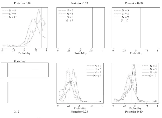
In Figure 1 we plot the distribution of mid-points for the intervals that contain our subjects’
risk neutral subjective probabilities. Each panel plots the distribution of average midpoints after
signals that differ in weight (N) and which are associated with a specific posterior. We have 6
posterior groups in total, 0.88, 0.77 and 0.6 when w>b, and by symmetry 0.12, 0.23 and 0.4 when
b>w. The vertical line in each panel shows the correct Bayesian probability. The distributions
shown in Figure 1 appear to be systematically related to the strength-weight characteristics of the
signals observed. In each posterior group the distributions related to larger dice samples appear to
have a lower mean, which implies that, holding the posterior constant, higher weight signals elicit
weaker responses, as predicted by GT.
In the next section we formally test the strength/weight hypothesis using a structural EUT
model which assumes that the bets with the different bookies are evaluated according to (1). Using
maximum likelihood we estimate the subjective probabilities and risk attitudes that best describe
subjects’ choices in both the risk and the belief task, and test whether the strength/weight
hypothesis is supported. To examine how assumptions about risk preferences affect inferences on
the bias we firstly estimate subjective probabilities assuming risk neutrality (RN), and then by
controlling for non-linear utility (SEU). The econometric details of the model are provided in
section D of the online Appendix.
III. Results
A. Experimental Results
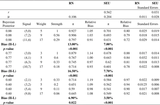
The top panel of Table 2 contains estimates for the coefficient of risk attitude, r, and the behavioral
error term, μ. 12 In the columns on the right side we have elicited subjective probabilities for different
models of choice (RN vs. SEU), along with their associated standard errors. Subjective probabilities
are grouped according to Bayesian posterior: 0.88, 0.77 and 0.6. To ease exposition we pool
subjective probabilities for symmetric patterns, i.e., (5,0) and (0,5).13The second column of Table
2 shows the composition of the signal, and the third and fourth
12The behavioral parameter μ is a structural “noise parameter” and is used to allow for some errors from the
perspective of the deterministic EUT model. Specifically μ>0 captures cases where the option with the lower
expected utility might be chosen by accident.
13 For example, if the subjective probability for the White estimated after a pattern of 5 white and 0 blue is π1 with
standard error σ(π1), and the probability for White elicited after a pattern of 0 white and 5 blue is π2 with standard error
columns show its strength and weight characteristics. In each panel the signals are arranged so that
as one goes further down the table weight increases and strength decreases.14
We start the discussion with the RN model. For the high strength/low weight signal (5,0)
we find overreaction, with elicited probability higher than the Bayesian posterior probability by
about 5%. The elicited probability then drops for the (7,2) signal to 90.6%, and drops even further
for the (11,6) signal to 79.7%. The hypothesis that these subjective probabilities are equal is safely
rejected (p-value <0.001). This pattern supports the original GT findings since subjective
probabilities increase with signal strength, in violation of Bayes Rule. To get a sense of the
magnitude of the bias we can subtract subjective probabilities associated with the (5,0) and (11,6)
signals, which yields 92.5% - 79.5% = 13%. We find similar patterns of the remaining groups of
0.77 and 0.6, with biases of 16.5% and 6.9% respectively, which are all statistically significant. 15
The column Relative Bias shows the corresponding bias associated with each probability as a
proportion of the required update from the prior of 0.5, and shows overreaction for low weight
signals and underreaction for high weight signals.
In the second model (SEU) the coefficient of risk attitude is equal to 0.562 and is highly
statistically significant, indicating risk aversion. The magnitude of risk aversion obtained is similar
to other experiments with similar stakes, reviewed in Harrison and Rutström (2008). As in the RN
case, subjective probabilities in all the Bayesian posterior groups increase with signal
14 We did not include in Table 2 dice combinations that emerged and that did not have equivalents in the original GT
(1992) design.
15 Kraemer and Weber (2004) also tested the GT effect, using stated preference methods of elicitation, using
hypothetical information signals. Their results were in line with the original GT findings, but did not allow a
comparison of the general magnitude of the bias since Kraemer and Weber (2004) restricted their analysis to
strength, and the differences between the high strength/low weight and low strength/high weight
probabilities are statistically significant. However, the striking result from this analysis is that once
we allow for risk aversion the magnitude of the bias halves. Specifically, for the 0.88 group the
bias is 7% instead of 13.0%, for the 0.77 group it is 7.7% instead of 16.5%, and for the 0.6 group
it is 3.5% instead of 6.9%. This highlights that inferences about the strength-weight effect under
the assumption of risk neutrality are likely to overstate the bias.16
How do our results compare to the original findings of GT? Across all three patterns the
average bias reported by GT is 20.6%.17 The corresponding average bias in our analysis is only
6.1% (p-value <0.001) when we allow for non-linear utility. The hypothesis that the average bias
in the two studies is equal is safely rejected (p-value <0.001). This comparison suggests that the
bias is significantly reduced when tested under experimental designs that incentivize responses,
which has important implications for inferences about the relevance of the strength-weight bias to
stock market anomalies.
GT report that their subjects overreact to high strength/low weight information, stating
probabilities that are higher than those implied by Bayes Rule. In our estimations we find
evidence of overreaction toward high strength/low weight signals only when we constrain r to
risk neutrality. When we allow for non-linear utility we find a general tendency of
underreaction, or conservatism (Edwards (1968)) toward sample information, as subjective
16 In unreported results we have derived results using a Rank Dependent Utility model, which accounts for both
non-linear utility and probability weighting via non-additive decision weights. The results show that our subjects do not
engage in probability weighting, therefore inferences regarding the strength-weight bias from this model are identical
to those drawn from the SEU model. These results are available from the authors upon request.
17 For the 0.88 case GT report a bias of 28% (92.5 - 64.5%), for the 0.77 a bias of 25.5% (85% - 59.5) and for the 0.6
probabilities are lower than Bayesian posterior probabilities (Relative Bias is less than 1 in all
cases). Moreover, in each posterior group underreaction is higher when the signal is of high weight.
For example, in the SEU model, for signals that imply a posterior of 0.88, underreaction is 25%
when the signal is of high weight (Relative Bias = 0.72) and 18% when it is of low weight (Relative
Bias = 0.8). This finding can provide an explanation for prices adjusting slowly to important, high
weight information such as earnings surprises (Bernard and Thomas (1989)) or changes to dividend
policy (Michaely et al. (1995)).
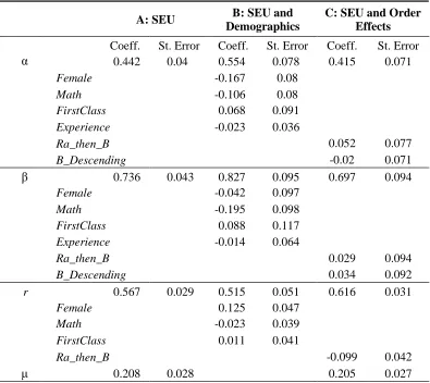
We continue to more formally test the strength/weight hypothesis by estimating the
following model: 18
(2) log {log(π/(1-π)) / log(0.6/0.4) } = α log N + β log S
Bayes Rule predicts that the coefficients on strength (β) and weight (α) should be both equal to
one, whereas β>α under the strength/weight hypothesis. The results, which are shown in panel A of Table 3, show that the coefficient on weight, α, is 0.442 and on strength, β, is 0.736, which
shows that signal strength affects probabilities more than signal weight, in line with our previous
results in Table 2. The hypotheses that α = β is safely rejected (p-value <0.001). We can define the
total bias as 1-α/β, equal to 40% in our data, again significantly smaller than the corresponding
bias of 62% reported by GT (p-value<0.001).19
We also use this model to test whether the strength-weight bias differs among subjects with
different demographic characteristics. Previous research found that female subjects are less likely
to behave as Bayesians in similar experimental tasks (Charness and Levin (2005)). We
18 This entails expressing the subjective probabilities within the structural model in terms of strength and weight,
and then estimating α and β using maximum likelihood. Section D of the online Appendix explains this procedure,
and section E derives (2) from Bayes Rule.
therefore condition estimates of α and /3 on the dummy Female. Moreover, subjects that have
knowledge of statistics have been found to behave more rationally in such quantitative tasks
(Halevy, 2007). To test for this effect we condition estimates of α and /3 on the dummy Math, which
takes the value if 1 if the subject is studying in a quantitative field. Subjects with higher cognitive
abilities have also been shown to act more rationally (Grinblatt, Keloharju, and Linnainmaa (2012)).
As a proxy for quantitative ability we define the proxy FirstClass, which takes the value of 1 if the
subject’s self-reported average marks to date are in the highest class.20Finally, experienced subjects
have been shown to act more rationally, both in experiments (Loomes, Starmer, and Sugden (2003))
and in the field (Seru, Shumway, and Stoffman (2010)). Although our experiment did not provide
any feedback it is possible that subjects learn about the latent process by observing which samples
are more or less frequent. To test for such learning we define the dummy Experience, which takes
the value of 1 for the last 15 rounds of the belief task, and 0 otherwise. We estimate the model in
(10) conditioning α and /3 on these dummies. We also condition r on Female, Math and FirstClass
as these variables may also affect risk attitudes.
The results are shown in Table 3 panel B. The entry next to each variable shows its marginal
contribution and its associated standard error. We find that females are significantly more risk
averse, consistent with prior studies. Females are found to be less sensitive to signal weight
(coefficient -0.167 with standard error 0.08), which suggests that their beliefs are more biased.
Subjects who study in quantitative fields respond less strongly to signal strength (coefficient -0.195
with standard error 0.098), which suggests that their beliefs are less biased. These effects are
statistically significant on the 5% level. Overall the analysis in panel B suggests that the
strength-weight bias is likely to be stronger among females and subjects with no
quantitative skills, but also that no group of subjects is completely immune to the strength-weight
effect.
Finally, we examine whether order effects influence our results by allowing estimates of α
and β to differ depending on whether the risk task was conducted first (RA_then_B = 1), and
depending on whether in the belief task the samples were presented in descending order (B_descen
= 1). We find that our estimates of α and β are not affected by order effects. However, we find that
subjects become more risk averse if the risk task is conducted first.
B. Asset Pricing Simulations
Our findings suggest that the strength-weight bias is weaker than reported by GT, and that subjects
are more likely to underreact rather than overreact. To examine the effect of these findings on asset
pricing, we re-calibrate the model proposed by Barberis et al. (1998) (BSV) to parameters that
imply such changes.
In BSV earnings are generated by a random walk process, but the investor falsely believes
in either a mean-reverting regime (underreaction) or a trending-regime (overreaction). There are
some probabilities that govern the transition from one model to the other, which can be thought to
relate to the strength-weight effect, i.e., the switch from underreaction to overreaction. The
investor observes past earnings realizations to determine which model is generating earnings; after
a short string of surprises of the same sign, which appear relatively ‘unconvincing,’ he
underreacts. As this string increases, and becomes more salient, he overreacts. BSV use this model
to simulate the returns of portfolios of firms with n consecutive positive or negative shocks (where
n ranges from 1 to 4), and show that the return differential
positive, indicating underreaction, turning negative for longer strings (n = 3, 4), indicating
overreaction.
Following this procedure we examine how changes in the transition probabilities, such
that the investor always relies more on model 1, affect
-
.21 We find that-decreases with n, but at a generally smaller rate. Moreover,
-
is larger for all n, and itrequires a longer string of news to actually turn it negative. Overall, our experimental findings, as
calibrated through the BSV model, imply more widespread underreaction in asset prices.
IV. Conclusion
Griffin and Tversky (1992) proposed the strength/weight hypothesis, which is that decision makers
are more responsive to the extremity (strength) of the information than to its predictive validity
(weight), even when both strength and weight are equally diagnostic. This hypothesis received
many applications in finance.
We tested whether the hypothesis holds by means of an experiment that allowed us to infer
subjective probabilities through betting decisions with real monetary incentives. We provide
respondents with imperfect information about the true state of the world, and ask them to reveal
their subjective belief about the likelihood of the true state by making a series of bets according to
the logic of Savage (1954, 1971) and Ramsey (1931).
Our results broadly support the original findings of GT, as decision makers generally
perceived events as more likely when the available evidence had high strength and low weight.
However, the magnitude of the bias we found was less than a third compared to that reported by
GT, which suggests that the impact of the strength-weight bias on stock market anomalies is likely
to be smaller than what the original estimates suggest.
References
Andersen, S.; J. Fountain; G. W. Harrison; and E. E. Rutström. “Estimating Subjective
Probabilities.” Journal of Risk and Uncertainty, 48 (2014), 207-229.
Andersen, S.; G. W. Harrison; M. I. Lau; and E. E. Rutström. “Discounting Behavior and the
Magnitude Effect: Evidence from a Field Experiment in Denmark.” Economica, 80(2013),
670-697.
Antoniou, C.; G. W. Harrison; M. I. Lau; and D. Read. “Subjective Bayesian Beliefs.”
Journal of Risk and Uncertainty, 50 (2015), 35-59.
Asparouhova, E.; M. Hertzel; and M. Lemmon. “Inference from Streaks in Random Outcomes:
Experimental Evidence on Beliefs in Regime Shifting and the Law of Small Numbers.”
Management Science, 55 (2009), 1766-1782.
Barberis, N.; A. Shleifer; and R. Vishny. “A Model of Investor Sentiment.” Journal of Financial
Economics, 49 (1998), 307-343.
Bernard, V. L., and J. K. Thomas. Post-Earnings-Announcement Drift: Delayed Price Response
or Risk Premium?” Journal of Accounting Research, 27 (1989), 1-36.
Bloomfield, R., and J. Hales. “Predicting the Next Step of a Random Walk: Experimental
Evidence of Regime-Shifting Beliefs.” Journal of Financial Economics, 65 (2002), 397414.
Bondarenko, O., and P. Bossaerts. “Expectations and Learning in Iowa.” Journal of Banking and
Cason, T. N., and C. R. Plott. “Misconceptions and Game Form Recognition of the BDM Method:
Challenges to Theories of Revealed Preference and Framing.” Journal of Political Economy,
122 (2014), 1235-1270.
Charness, G.; E. Karni; and D. Levin. “Individual and Group Decision Making Under Risk: An
Experimental Study of Bayesian Updating and Violations of First-Order Stochastic
Dominance.” Journal of Risk and Uncertainty, 35(2007), 129-148.
Conlisk, J. (1989). “Three Variants on the Allais Example.” American Economic Review, 79
(1989), 392-407.
Costa-Gomes, M. A., and G. Weizsäcker. “Stated Beliefs and Play in Normal-Form Games.”
Review of Economic Studies, 75 (2008), 729-762.
Daniel, K., and S. Titman. “Market Reactions to Tangible and Intangible Information.” Journal of
Finance, 61 (2006), 1605-1643.
Edwards, W. “Conservatism in Human Information Processing.” In Formal Representation of
Human Judgment, B. Kleinmutz, eds. Wiley, New York, (1968).
Ellsberg, D. “Risk, Ambiguity, and the Savage Axioms.” Quarterly Journal of Economics, 75
(1961), 643-669.
de Dreu, J., and J. A. Bikker. “Investor Sophistication and Risk Taking.” Journal of Banking &
Finance, 36 (2012), 2145-2156.
Fiore, S. M.; G. W. Harrison; C. E. Hughes; and E. E. Rutström. “Virtual Experiments and
Environmental Policy.” Journal of Environmental Economics and Management, 57 (2009),
Charness, G., and D. Levin (2005). “When Optimal Choices Feel Wrong: A Laboratory Study of
Bayesian Updating, Complexity, and Affect.” American Economic Review, 95 (2005),
1300-1309.
Gilboa, I.; A. W. Postlewaite; and D. Schmeidler. “Probability and Uncertainty in Economic
Modeling.” Journal of Economic Perspectives, 22 (2008), 173-188.
Grether, D. M. “Bayes Rule as a Descriptive Model: The Representativeness Heuristic.” Quarterly
Journal of Economics, 95 (1980), 537-557.
Griffin, D., and A. Tversky. “The Weighing of Evidence and the Determinants of Confidence.”
Cognitive Psychology, 24 (1992), 411-435.
Grinblatt, M.; M. Keloharju; and J. Linnainmaa. J. “IQ, Trading Behaviour, and Performance.”
Journal of Financial Economics, 104 (2012), 339-362.
Gupta-Mukherjee, S. “Investing in the ‘New Economy’: Mutual Fund Performance and the Nature
of the Firm.” Journal of Financial and Quantitative Analysis, 49 (2013), 1-42.
Hackbarth, D. “Determinants of Corporate Borrowing: A Behavioral Perspective.” Journal of
Corporate Finance, 15 (2009), 389-411.
Halevy, Y. “Ellsberg Revisited: An Experimental Study.” Econometrica, 75 (2007), 503-536.
Harrison, G. W.; E. Johnson; M. M. McInnes; and E. E. Rutström. “Risk Aversion and Incentive
Effects: Comment.” American Economic Review, 95 (2005), 897-901.
Harrison, G. W., and E. E. Rutström. “Risk aversion in the Laboratory.” In Risk Aversion in
Hey, J. D., and C. Orme. “Investigating Generalizations of Expected Utility Theory Using
Experimental Data. Econometrica, 62 (1994), 1291-1326.
Kadane, J. B., and R. L. Winkler. “Separating Probability Elicitation from Utilities.” Journal of the
American Statistical Association, 83 (1988), 357-363.
Kraemer, C., and M. Weber. “How do People Take Into Account Weight, Strength and Quality of
Segregated vs. Aggregated Data? Experimental Evidence.” Journal of Risk and Uncertainty,
29 (2004), 113-142.
Kuhnen, C. M. “Asymmetric Learning from Financial Information.” Journal of Finance, (2015)
Forthcoming.
Kuhnen, C. M., and B. Knutson. “The Influence of Affect on Beliefs, Preferences, and Financial
Decisions.” Journal of Financial and Quantitative Analysis, 46 (2011), 605-626.
Laury, S. K.; M. M. McInnes; and J. T. Swarthout. “Insurance Decisions for Low-Probability
Losses. Journal of Risk and Uncertainty, 39 (2009), 17-44.
Liang, L. “Post-Earnings Announcement Drift and Market Participants' Information Processing
Biases.” Review of Accounting Studies, 8 (2003), 321-345.
Loomes, G.; C. Starmer; and R. Sugden. “Do Anomalies Disappear in Repeated Markets?”
Economic Journal, 113 (2003), 153-166.
Michaely, R.; R. H. Thaler; and K. L. Womack. “Price Reactions to Dividend Initiations and
Omissions: Overreaction or Drift?” Journal of Finance, 50 (1995), 573-608.
Plott, C. R., and K. Zeiler. “The Willingness to Pay–Willingness to Accept Gap.” American
Puetz, A., and S. Ruenzi. “Overconfidence Among Professional Investors: Evidence from Mutual Fund Managers.” Journal of Business Finance & Accounting, 38 (2011), 684-712.
Ramsey, F. P. “Truth and probability. The Foundations of Mathematics and Other Logical Essays.”
Routledge and Kegan Paul, London, 1931.
Rutström, E. E., and N. T. Wilcox. “Stated Beliefs Versus Inferred Beliefs: A Methodological
Inquiry and Experimental Test.” Games and Economic Behavior, 67 (2009), 616-632.
Savage, L. J. “The Foundations of Statistics.” New York: Wiley, (1954).
Savage, L. J. “Elicitation of Personal Probabilities and Expectations.” Journal of the American
Statistical Association, 66 (1971), 783-801.
Seru, A.; T. Shumway; and N. Stoffman. “Learning by Trading.” Review of Financial Studies, 23
(2010), 705-739.
Smith, V. L. “Microeconomic Systems as an Experimental Science.” American Economic Review,
72 (1982), 923-955.
Sorescu, S., and A. Subrahmanyam. “The Cross Section of Analyst Recommendations.” Journal
N = 5 N = 9 N=17
N = 3 N = 5 N = 9 N=17
[image:23.792.142.666.135.518.2]N = 3 N = 5 N = 9 N=17
Figure 1: The Distribution of Switch Points for Different Signals with the Same Posterior
This figure present the distribution of risk-neutral probabilities, grouped according to Bayesian Posterior (6 cases) and signal weight (number
of dice rolled, N). The vertical black line in each Panel depicts the Bayesian Probability.
Posterior 0.88 Posterior 0.77 Posterior 0.60
0 .25 .5 .75 1
Probability 0 .25 Probability .5 .75 1
Posterior
0.12 Posterior 0.23 Posterior 0.40
N = 5
0 .25 .5 .75 1
Probability
N = 3 N = 5 N = 9 N=17
0 .25 .5 .75 1
Probability 0 .25 Probability .5 .75 1 N = 3
0 .25 .5 .75 1 Probability
Table 1: The Betting Sheet Used by the Subjects
This table shows the betting sheet that subjects used to place their bets (a non-transferrable stake of £3 for each bookie)
after each signal. The Table lists 19 hypothetical bookies which offer different odds on the white or blue box being
Table 2: Estimated Subjective Probabilities
This table reports subjective probabilities and preference parameters estimated with maximum likelihood. Subjective probabilities are
constrained to lie in the unit interval, using the transform π = 1/(1+exp(κ)), where κ is the parameter estimated and π is the inferred probability.
We report the average probability elicited after symmetric signals (e.g., (5,0) and (0,5)), using the delta method to estimate the standard error
for pooled π from estimates of κ. We employ “frequency weights” of 50 for every observed choice from the risk task to ensure that the
estimated risk parameters are based primarily on the choices from the risk tasks. In the RN column, which stands for Risk Neutral, we
estimate the model assuming risk neutrality (constraining r=0.0001). In the SEU column we remove this constraint and allow risk aversion,
assuming a CRRA utility function of the type y1-r/(1-r). μ is a structural error parameter and π is the subjective probability. Relative Bias is
calculated as π/Bayesian Posterior. The last two columns indicate the standard errors of estimated parameters (r, μ and π) using the delta
method. Standard errors are also clustered on the subject level. The econometric procedure employed is explained in detail in section D of
the online Appendix.
RN SEU RN SEU
Standard Errors r μ 0.106 0.562 0.204 0.011 0.031 0.028 Bayesian
Posterior Signal Weight Strength π
Relative
Bias π
Relative
Bias Standard Errors
0.88 (5,0) 5 1 0.927 1.05 0.701 0.80 0.025 0.019
0.88 (7,2) 9 0.56 0.906 1.03 0.693 0.79 0.018 0.015
0.88 (11,6) 17 0.29 0.797 0.91 0.631 0.72 0.029 0.014
Bias (H-L) 13.00% 7.00%
p-value <0.001 <0.001
0.77 (3,0) 3 1 0.879 1.14 0.678 0.88 0.017 0.014
0.77 (4,1) 5 0.6 0.767 1.00 0.643 0.84 0.032 0.011
0.77 (6,3) 9 0.33 0.745 0.97 0.62 0.81 0.018 0.013
0.77 (10,7) 17 0.18 0.714 0.93 0.601 0.78 0.022 0.008
Bias (H-L) 16.50% 7.70%
p-value <0.001 <0.001
0.60 (2,1) 3 0.33 0.714 1.19 0.584 0.97 0.022 0.009
0.60 (3,2) 5 0.2 0.651 1.09 0.562 0.94 0.0125 0.006
0.60 (5,4) 9 0.11 0.59 0.98 0.541 0.90 0.017 0.007
0.60 (9,8) 17 0.06 0.645 1.08 0.549 0.92 0.021 0.008
Bias (H-L) 6.90% 3.50%
Table 3: The Effect of Strength and Weight on Subjective Probabilities
This table reports estimates for the model in Equation 2 with maximum likelihood. In Panel A we assume an SEU
representation with a CRRA utility function as in Table 2. In Panels B and C we use the same CRRA representation and
examine the role of demographics and experimental procedures, respectively. Specifically we define the dummy variable
Female, which takes the value of 1 if the subject is female, Math, which takes the value of 1 if the subject is majoring
in Economics, Finance, Engineering, Physical or computer sciences, First_Class which takes the value of one if the
subject’s marks to date are higher than 70%. The dummy Experience takes the value of 1 for the last 15 samples in the
belief task. Ra_then_B is equal to 1 if the risk task was conducted first and B_Descending is equal to 1 if the samples in
the belief task were presented in descending order. In Panel B (C) we condition α and β on the demographic
(experimental design) dummies. μ is a structural error parameter. Standard errors are clustered on the subject level. The
econometric procedure employed is explained in detail in section D of the online Appendix.
A: SEU B: SEU and
Demographics
C: SEU and Order Effects Coeff. St. Error Coeff. St. Error Coeff. St. Error
α 0.442 0.04 0.554 0.078 0.415 0.071
Female -0.167 0.08
Math -0.106 0.08
FirstClass 0.068 0.091
Experience -0.023 0.036
Ra_then_B 0.052 0.077
B_Descending -0.02 0.071
β 0.736 0.043 0.827 0.095 0.697 0.094
Female -0.042 0.097
Math -0.195 0.098
FirstClass 0.088 0.117
Experience -0.014 0.064
Ra_then_B 0.029 0.094
B_Descending 0.034 0.092
r 0.567 0.029 0.515 0.051 0.616 0.031
Female 0.125 0.047
Math -0.023 0.039
FirstClass 0.011 0.041
Ra_then_B -0.099 0.042
Online Appendix to “Information Characteristics and Errors in Expectations: Experimental Evidence”
A. Subject Demographics
Age Mean Median
21.3 20
Sex
Male 58
Female 53
Field
Economics, Finance, Business Administration 24
Engineering 4
Biological sciences, Health Medicine 6 Math, Computer or Physical Sciences 26
Social Sciences 23
Law 8
Psychology 4
Modern Languages 8
Other fields 8
Level of study
Undergraduate 88
Postgraduate 12
Graduate 11
Mark at Bachelor degree
Above 70% (first class) 30
between 60 and 69% (2.1) 72
between 50 and 59% (2.2) 5
B. Instructions for the Belief Task
In this stage of the experiment you will be betting on the outcomes of uncertain events. Usually we bet on events like football matches or elections, but in this task the events will be random choices made by the experimenter between two boxes, one blue and the other white. The experimenter will not tell you which box was chosen. At the start each box will have the same chance of being chosen, but once it has been chosen the experimenter will give you some information to help you work out the chances that it was blue or white. Armed with this information, you will make bets on which box was chosen.
The procedure, which is summarized on the accompanying picture, is as follows. The
experimenter will first choose the box by rolling a 6-sided die with three blue and three white sides. If blue comes up he will choose the blue box, if white comes up he will choose the white one.
Both the white and blue boxes contain several dice, each having 10 sides. Both boxes have the same number of dice, which will vary over the course of the experiment. The dice in the blue box always have 6 blue sides and 4 white ones, while those in the white box have 4 blue sides and 6 white ones.
The experimenter will roll all the dice in the chosen box and tell you how many blue and white sides came up. He will not tell you which box was chosen.
Because the dice in the blue box have more blue sides than those in the white box, knowing the number of blue and white sides that come up can help you work out the chances that each box was chosen. For example, if more blue sides come up this means it is more likely to be the blue box, and if more white sides come up it is more likely to be the white box.
Once you have the information about the dice rolls, you will then make bets on which box was chosen.
About betting
You will be making bets with several betting houses or “bookies,” just as you might bet on a football game or a horse race.
Imagine a two horse race between Blue Bird and White Heat. Several bookies offer different odds for both horses. The table below shows the odds offered by three bookies along with the amounts they would pay if you staked £10 on the winning horse. The earnings are calculated by multiplying the odds by the stake. In this experiment you will be making bets on which box was chosen using a table like this. At this point you should take some time to study the table.
Bookie Stake
Odds offered
Earnings including the stake of £10
Blue Bird White Heat Blue Bird White Heat
A £10 5.00 1.25 £50.00 £12.50
B £10 3.33 1.43 £33.33 £14.30
C £10 2.00 2.00 £20.00 £20.00
Below are three important points about betting.
1. Your belief about the chances of each outcome is a personal judgment that depends on information you have about the different events. For the horse race, you may have seen previous races or read articles about them. In the experiment the information you have about whether the blue or white box was chosen will be how many blue and white faces came up.
2. Even if you believe Event X is more likely to occur than Event Y, you may want to bet on Y because you find the odds attractive. For example, even if you believe White Heat is most likely to win you may want to bet on Blue Bird because you find the odds attractive. To illustrate, suppose you personally believe that Blue Bird has a 40% chance of winning and White Heat has a 60% chance of winning. This means that if you bet £10 on Blue Bird with Bookie A you believe there is a 40% chance of receiving £50.00 and a 60% chance of receiving nothing. You may find this more attractive than betting on White Heat, which you believe offers a 60% chance of 12.50 and a 40% chance of nothing.
3. Your choices might also depend on your willingness to take risks or to gamble. There is no right choice for everyone. In a horse race you might want to bet on the long-shot since it will bring you more money if it wins, but you also might want to bet on the favourite since it is more likely to win something.
Your choices
Now you are familiarized with odds, we can go back to the experimental betting task. Recall that the experimenter will first make a random choice of a blue or white box. Then he will roll the dice in the chosen box and tell you how many white and blue sides came up. Then you will consider the chances that the box chosen was blue or white, and make a series of bets.
You have a booklet of record sheets. Each record sheet shows the bookies you will be dealing with, and the odds they offer. There are 19 bookies on each sheet, and each offer different odds for the two outcomes. Take a minute to look at one such record sheet, shown on the next page.
There will be 30 separate events, and 19 bookies offer odds for each event. You will make bets at all 19 bookies for all 30 events.
For each bet, you have a £3 stake, and the record sheet shows the payoffs you will receive if you bet on the box that was actually chosen.
There is a separate record sheet for each of the 30 events. On each sheet you should circle W or B to indicate the bet you want to make with all 19 bookies.
One and only one of the bets in the entire experiment will pay off for real. Therefore, please consider each bet as if it is the only one that will be paid out. After you have placed all your bets, you will roll a 30-sided die to determine which event will be played out, and a 20-sided die to determine which bookie will determine your earnings.
C. Instructions for the Risk Elicitation Task
This stage is about choosing between lotteries with varying prizes and chances of winning. You will be shown a series of 20 lottery pairs, and you will choose the lottery you prefer from each pair. You will actually get the chance to play one of the lotteries you choose, and will be paid according to the outcome of that lottery, so you should think carefully about your preferences.
Here is an example of one lottery pair. You will have to think about which lottery you would prefer to play and tick the appropriate box below
The outcome of the lotteries will be determined by the draw of a random number between 1 and 100. We will ask you to roll a 100-sided die that is numbered from 1 to 100, and the number on the die will determine the outcome of the lotteries.
In the above example the left lottery pays five pounds (£5) if the number on the die is between 1 and 40, and it pays fifteen pounds (£15) if the number is between 41 and 100. The light green segment of the pie chart corresponds to 40%, and the orange segment corresponds to 60% of the area.
Each of the 20 lottery pairs will be shown on a separate sheet of paper. On each sheet you should indicate your preferred lottery by ticking the appropriate box. After you have worked through all the lottery pairs, please raise your hand. You will then roll a 20-sided die to determine which pair of lotteries will be played out, and then roll the 100-sided die to determine the outcome of the chosen lottery.
For instance, suppose you picked the lottery on the left in the above example. If you roll the 100-sided die and the number 37 is shown, you would win £5; if it was 93, you would get £15. If you picked the lottery on the right and drew the number 37, you would get £5; if it was 93, you would get £15.
Therefore, your payoff is determined by three things:
which lottery pair is chosen to be played out using the 20-sided die;
which lottery you selected, the left or the right, for the chosen lottery pair; and the outcome of that lottery when you roll the 100-sided die.
This is not a test of whether you can pick the best lottery in each pair, because none of the lotteries are necessarily better than the others. Which lotteries you prefer is a matter of personal taste.
Please work silently, and think carefully about each choice.
D. The Structural Model
We start by explaining the econometric analysis of the data collected in the risk task. We assume a CRRA utility function in the context of EUT, shown by (1) in the main text of the paper, where r
is a parameter to be estimated, and y is income from the experimental choice. The utility function (1) can be estimated using the responses from our risk task using maximum likelihood and a latent EUT structural model of choice. In the lotteries provided there are K possible outcomes, therefore, Expected Utility (EU) of each lottery i is:
EUi = k=1,K [ pk
x
uk ]. (1)The EU for each lottery pair is calculated for a candidate estimate of r, defining the index:
V
EU = EUR - EUL (2)This latent index is linked to the observed choices using a standard cumulative normal distribution function Φ(VEU), resulting to a probit link function:
prob(choose lottery R) = Φ(
V
EU) (3)An important extension of the core model is to allow for respondents to make some errors. We use the contextual error specification proposed by Wilcox (2011). It posits the latent index:
prob(choose lottery R) = Φ [ (
V
EU)/v)/μ ](4)
where v is a normalizing term for each lottery pair L and R, defined as the maximum utility over all prizes in this lottery pair minus the minimum utility over all prizes in this lottery pair. μ>0 is a structural “noise parameter” used to allow some errors from the perspective of the deterministic EUT model. As μ
-*
this specification collapsesV
EU to 0 for any values of EUR and UL, so theprobability of either choice converges to 1/2. Therefore, a larger μ means that the difference in the
EU of the two lotteries, conditional on the estimate of r, is less predictive of choices. In our estimations we use a log-transform for μ to ensure that it is non-negative, with standard errors and point estimates derived using the delta method. Additional details of the estimation methods used, including corrections for “clustered” errors when we pool choices over respondents and tasks, are provided by Harrison and Rutström (2008).The log-likelihood is then:
ln L(r,
t
; y, X) = i [ (ln Φ(V
EU)x
I(yi = 1)) + (ln (1-Φ(V
EU))x
I(yi = -1)) ] (5)where I(
.
) is the indicator function, yi =1(-1) denotes the choice of the Option R (L) lottery in riskEUW = πw U(payout if W | bet on W) +
(1-πw) U(payout if B | bet on W) (6)
where irw is the subjective probability that W will occur. The payouts that enter the utility function are defined by the odds that each bookie offers. The EU received from a bet on event B is defined similarly.
We observe the bet made by the subject for a range of odds, so we can calculate the likelihood of that choice given values of r, irw and p, again assuming EUT and CRRA. The rest of the structural specification is exactly the same as for the choices over lotteries with objective probabilities. Thus the likelihood function for the observed choices in the belief task is:
ln L(r, πw, μ; y, X) = i [ (ln Φ( EU) I(yi = 1)) + (ln (1-Φ( EU)) I(yi = -1)) ] (7)
The joint estimation problem is to find values for r, irw and p that maximize the sum of (5) and (7). To ensure that the choice probability lies in the unit interval we use the transform ir = 1/(1+exp(κ)), where κ is the parameter estimated which is free to vary between ±∞ and π is the inferred probability. To infer point estimates and standard errors for ir from estimates of κ we again use the delta method.
To formally examine the sensitivity of subjective probabilities to strength, S, and weight,
N, we can estimate the following model:
log {log(ir/(1-ir)) / log(0.6/0.4) } = α log N + fl log S (8)
where ir and 1- ir are the elicited subjective probabilities for White or Blue, respectively. Bayes Rule implies that α= fl=1, but under the strength-weight hypothesis α < fl. Because, generalizing GT, we obtain both w>b and b>w cases, we make a transformation to the definition of the subjective probability in the model, to ensure that strength S is always positive. Thus when w>b we express it as π = 1/(1+(1/λ)), and when b<w we express it as π = 1/(1+λ), where λ = exp[ exp(γ) exp(0.6/0.4)
].
E. Derivation of Equation 2
Here we provide the general procedure for computing the posterior probability that a given set of dice (White or Blue, W or B) was chosen given the sample outcome (w,b). The posterior probability, Jr, that W was chosen is:
( | )
( | ) ( )( ) .
The posterior probability of B is then 1- Jr. The likelihoods are the probabilities of given data, in this case (w,b), given the hypothesis, in this case W or B. The likelihood of W and B are therefore:
p(w,b|W) = [N!/(w! b!)] p(W)w (1-p(W)) b,
p(w,b|B) = [N!/(w! b!)] p(B)w (1-p(B)) b,
The odds ratio is p(w,b|W)/p(w,b|B) which taking into account the fact that p(B) = 1-p(W), reduces with some simple algebra to the following:
(
( ) | | .( )
)
To separate out the effects of strength and weight we first take the log on both sides of the equation and then multiply and divide through by N:
( ) |
|
(
( )( ))
(| |) (
( )( ))
Re-arranging and taking again the log on both sides gives the expression for weight and strength from Griffin and Tversky (1992):
( ( )⁄
(
( )(
)) )
( )
(⌊⌋)
Multiplying the two right-hand terms by α and β, respectively, we generate expression (17) from our paper:
( ( )
(
( )⁄
( )))
( )
(| |)
F: Asset Pricing Simulations
In this table we report results from simulations using the procedure in Barberis, Shleifer and Vishny (1998). Specifically, we use this model to simulate a string of n=6 earnings shocks for 2,000 companies, using a random walk model. All firms have initial earnings equal to N1, and then in each of the following periods all firms are
equally likely to experience a positive or negative earnings shock equal to y. Following BSV, we choose y to be low relative to N1 to avoid having negative earnings, and hence negative prices. Prices are derived according to Proposition 1 in BSV. We form two portfolios in each period: one consisting of firms with a positive earnings surprise in each of the n years, where n ranges from 1 to 4, and another with firms with a negative earnings shock. We then calculate the returns of these portfolios in the following year, and
report the difference . Returns are in percent. The focus of our analysis is to examine how changes in the transition probabilities, A1 and A2, affect the signs of returns. In the column titled BSV we present results
with A1=0.1 and A2=0.3, following BSV. In the remaining three columns we change these parameters by the
indicated percentage in a way that implies that the investor is always more likely to rely on the mean-reverting regime to forecast earnings (i.e., decreasing A1 and increasing A2), and repeat the process, holding all other
parameters constant.
n BSV 10% change 20% change 30% change
1.00 2.61 3.61 4.36 5.02
2.00 0.66 1.96 3.17 4.24
3.00 -2.27 0.22 1.60 3.20
References