Coverage Analysis of Multi Stream MIMO HetNets with MRC Receivers

For Peer Review

Coverage Analysis of Multi-Stream MIMO HetNets with MRC Receivers

Journal: IEEE Transactions on Wireless Communications

Manuscript ID Paper-TW-Mar-17-0285

Manuscript Type: Original Transactions Paper

Date Submitted by the Author: 06-Mar-2017

Complete List of Authors: Khoshkholgh, Mohammad; The University of British Columbia, EECE; Navaie, Keivan; Lancaster University, School of Computing and Communications

Shin, Kang G. ; University of Michigan, EECS

Leung, Victor; The University of British Columbia, Electrical and Computer Engineering

Keyword:

For Peer Review

Coverage Analysis of Multi-Stream MIMO HetNets

with MRC Receivers

Mohammad G. Khoshkholgh, Keivan Navaie, Senior Member, IEEE,

Kang. G. Shin, Life Fellow, IEEE, Victor C. M. Leung, Fellow, IEEE

Abstract

Most of current research on the coverage performance of multi-stream MIMO heterogeneous

networks (HetNets) has been focusing on a single data-stream. This does not always provide accurate

results as our analysis shows the cross-stream correlation due to interference can greatly affect the

coverage performance. This paper analyzes the coverage probability in such systems, and studies the

impact of cross-stream correlation. Specifically, we focus on the max-SIR cell association policy, and

leverage stochastic geometry to study scenarios whereby a receiver is considered in the coverage, if all

of its data-streams are successfully decodeable. Assuming open-loop maximum ratio combining (MRC)

at receivers, we consider cases where partial channel state information is available at the receiver. We

then obtain an upper-bound on the coverage and formulate cross-stream SIR correlation. We further

show that approximating such systems based on fully-correlated (non-correlated) data-streams, results

in a slight underestimation (substantial overestimation) of the coverage performance. Our results provide

insights on the multiplexing regimes where densification improves the coverage performance. We also

compare MRC with more complex zero-forcing receiver and provide quantitative insights on the design

trade-offs. Analysis is validated via extensive simulations.

Index Terms

Manuscript received March 06, 2017. Part of this work has been presented in the IEEE VTC-F 2016, Montreal [1].

M. G. Khoshkholgh and V. C. M. Leung ([email protected],[email protected]) are with the Department of

Electrical and Computer Engineering, the University of British Columbia, Vancouver, BC, Canada V6T 1Z4; K. Navaie

([email protected]) is with the School of Computing and Communications, Lancaster University, Lancaster, UK LA1

4WA; K. G. Shin ([email protected]) is with the Department of Electrical Engineering and Computer Science, University of

Michigan, Ann Arbor, MI 48109-2121, U.S.A.

For Peer Review

Densification, heterogeneous networks (HetNets), multiple-input multiple-output (MIMO),

multi-plexing gain, network-wise coverage performance, signal-to-interference ratio (SIR) correlation,

stochas-tic geometry.

I. INTRODUCTION

Spectral efficiency in heterogenous networks (HetNets) is substantially enhanced using den-sification and universal frequency reuse. A key physical-layer component of dense HetNets is MIMO technology which is also capable of meeting the high demand for wireless bandwidth [2, 3]. Nevertheless, macroscopic (network-level) performance, where MIMO multiplexing com-munication is utilized in conjunction with densification and heterogeneity, still remains to be explored.

Conventionally, MIMO systems are analyzed for isolated scenarios, where only point-to-point, single cell, and/or clustered communications are considered [4, 5]. Such analyses can characterize the various design aspects of MIMO HetNets, but they cannot capture the macroscopic perfor-mance of MIMO systems under severe and heterogenous inter-cell interference (ICI), commonly seen in dense HetNets with aggressive frequency reuse. We would like to address this very issue by using stochastic-geometry-based analytical techniques.

Stochastic geometry has been widely used for modeling and performance evaluation of wireless cellular networks, including HetNets, e.g., [6–10]. Using these techniques enables incorporation of impacts of line-of-sight propagation, path-loss models, and blockage effect into the network-wise evaluation of spectral efficiency without compromising the tractability and accuracy of the analysis [8, 10, 11].

A. Related Work

Reviewed below are the related studies of the performance of MIMO systems. The adopted cell-association (CA) policy plays a crucial role in the performance of MIMO HetNet systems. In a given coverage area, cell association determines which BS to serve a given mobile user. Different CA approaches are categorized as range expansion and Max-SIR association.

The range expansion policy uses maximum average received power as the association criterion. The coverage probability and area spectral efficiency (ASE) of multiple-input single-output

For Peer Review

(MISO) space-division multiple access (SDMA) systems utilizing this CA policy has been investigated in [12, 13]. The merits of interference cancellation in zero-forcing (ZF) based receive filters in enhancing the coverage of cellular systems was also demonstrated in [14]. Further, in [15–20] design issues, impacts of beamforming schemes, and antenna selection techniques on ASE, coverage, and energy-efficiency of MIMO communications with range extension CA were investigated [15–17]. Optimized offloading for controlling ICI utilizing coordinated MIMO communications was carried out in [18]. Coverage probability, spectral efficiency, and load balancing in MIMO systems are also considered in [19]. To improve the performance of range expansion in MIMO systems, the authors of [20] proposed a threshold-based CA solution.

With multi-antenna receivers, the authors of [21, 22] focused on maximum ratio combining (MRC) and optimal combining in the downlink and uplink, respectively. Applying Gil-Pelaez inversion theorem in [11], the symbol error probability (SEP) of MIMO multiplexing systems was analyzed in [23]. Equivalent-in distribution (EiD) was also developed in [24] to quantify error probability. Adopting the proposed framework of [24], a unified method for studying outage probability in MIMO communications was then proposed in [25].

In general, range-expansion CA does not distinguish between the corresponding MIMO tech-niques in the CA stage. So, in many cases mentioned above, the CA policy is in fact a replica of the one considered in the SISO counterpart [7, 9]. This makes range expansion defiant in effectively incorporating the attributes of MIMO communications to improve multiplexing and diversity. That is one of the reasons why heuristic offloading procedures are often required to optimize the system performance [13, 18, 20].

Nevertheless, the coverage is directly related to signal-to-interference (SIR) distribution. In addition, many network management functions, such as handover and fractional frequency reuse, often operate based on the SIR (or a function thereof) as the main decision metric. These justify consideration of CA rules based on the SIR characteristics.

The authors of [6, 26, 27] considered max-SIR CA in which the serving BS is the one that provides the maximum SIR. For MISO systems, the authors of [28] provided ordering results on the coverage, capacity, and ASE, and compared several beamforming techniques. In [29],

For Peer Review

we proposed a flexible max-SIR CA rule tailored for MISO-SDMA systems. Algorithms for specifying the number of required SIR measurements before choosing the supporting BS in order to optimize the coverage probability/spectral efficiency were also developed in [29].

Unlike the range-expansion technique for which various aspects of coverage performance have been investigated, the coverage performance of multi-stream MIMO-MRC communications with max-SIR CA is yet to be explored. The main objective of this paper is to analyze the coverage performance of MIMO communication with max-SIR CA rule, where multiple streams are transmitted at the same time. Note that in the literature of multi-stream MIMO communications, the coverage probability of the network is often estimated from the perspective of a given data stream. The thus-obtained coverage for a given data stream is then treated as the coverage performance of the multiplexing (multi-stream) system, see, e.g., [21, 30–33]. Nevertheless, such approach may cause substantial error in the evaluation of the coverage probability of multi-stream MIMO HetNets, as the possible correlation across data streams are entirely overlooked.

In fact, when the SIR values among data streams are correlated, the stream-level performance that considers the reception quality of a single data stream independent from the others, becomes inadequate. This is because the successful decoding of a data stream is partially dependent upon the decoding status of other data streams. Therefore, the coverage performance of MIMO multiplexing systems from a link-level perspective that considers the reception of all the data steams becomes crucial. In our previous works, [1][49][34], we studied the coverage probability of MIMO multiplexing systems from a link-level perspective. In [49] the focus was on multi-stream MIMO systems where the pre-coding and decoding filters at the transmitter and receiver was constructed according the singular value decomposition (SVD) technique. This techniques however requires perfect and timely CSI at both the transmitter and receiver, which imposes high signaling overhead particularly in dense configurations. Furthermore, in [34], we investi-gated the link-level coverage performance for multi-stream MIMO networks with zero-forcing beamforming (ZFBF) receivers. The simulation results in [34] show subtle differences between link-level, and stream-level coverage performance in a multi-stream MIMO system. Despite its importance, to the best of our knowledge, the roots and scales of such a discrepancy has not yet

For Peer Review

been investigated in the related literature.

On the other hand, in SIMO ad hoc networks, the ICI is shown to result in a high correlation among impinged signals across different receive antennas, see, e.g., [35, 36]. Such a correlation compromise the otherwise achievable diversity gain in cases where signals across antennas are independent. This is because in the presence of ICI, the path-loss fluctuations invoke (statistically) correlated interference among antennas due to the common locations of interferers. A similar conclusion was drawn in [21], where the interference correlation was investigated in space-time MIMO ad hoc networks. It was also shown in [21] that ignoring interference correlation among antennas may, in some cases, substantially compromise the accuracy of the analysis. The analysis in [21] is, however, limited to the CDF distribution of an individual data stream, thus being unable to depict the impact of correlation on the CDF distribution of a communication link with a set of data streams.

B. Contributions and Organization

In this paper, we investigate cross-stream SIR correlation and its impacts on the link-level coverage probability in MIMO multiplexing systems. We mainly focus on the maximum ratio combining (MRC) receivers. Note that compared to the ZFBF, the coverage evaluation of the MRC is more challenging due to the cross-stream interference. The coverage performance of MIMO-MRC systems from the stream-level perspective is studied in the context of ad hoc communications, e.g., [32]. The results in an ad hoc context are not necessarily extendable to cellular networks because, unlike cellular systems, ad hoc communications often operate without a CA mechanism and lack a central scheduler.

Here we evaluate the MIMO-MRC coverage probability from a link-level perspective in cellular networks. Despite the popularity and practical significance of an MIMO-MRC system for cellular communications due to its simple implementation and near zero feedback overheads, its performance in HetNet settings has not yet been investigated. Our model and analysis are concerned with scenarios that channel state information (CSI) is not available at the BSs and only partially known at the UEs. This paper makes the following two main contributions.

For Peer Review

• We obtain a closed-form and easy-to-compute tight upper bound on the network coverage probability for cases where successful decoding of all transmitted data streams is required. The unique feature of our analysis is to accurately incorporate SIR correlation. Our analytical results—supported by extensive simulations—provide significant practical insights on the impacts of densification on the link-level coverage performance. Based on this result, we conclude that improvement in the network coverage performance by densification is subject to careful selection of multiplexing gains in different tiers.

• We also analyze the cross-stream SIR correlation amongst multiple streams in a communica-tion link. Our analysis provides quantitative insights on the impact of tiers’ BSs density, path-loss exponent, CSI inaccuracy, and multiplexing gains on the SIR correlation among data streams. To understand the impacts of SIR correlation on the coverage probability, we then obtain the closed-form bounds on the coverage probabilities for two extreme settings: full SIR correlation (FC) among data streams, and no SIR correlation (NC) among data streams. We then show that the NC setting substantially over-estimates the coverage performance while the FC setting slightly underestimates it.

The rest of the paper is organized as follows. Section II presents the system model and Section III provides coverage evaluation. Section IV investigates the SIR correlation and its impact on the coverage probability. The simulation results are provided in Section V followed by conclusions in Section VI.

II. SYSTEMMODEL

We consider the downlink in a heterogeneous cellular network (HetNet) consisting of K ≥1 tiers of randomly located base-stations (BSs). In each tier i ∈ K, BSs are spatially distributed according to a homogenous Poisson Point Process (PPP), Φi, with a given spatial density, λi ≥

1 [6]. For mathematical tractability, we assume that the PPPs corresponding to each tier are mutually independent. Therefore, each tier i can be completely characterized by the spatial density of its BSs, λi, their transmit power, Pi Watts, the corresponding SIR threshold at the

receivers, βi ≥ 1, the number of BS’s transmit antennas Nit, and the number of scheduled

streams Si ≤min{Nit, Nr} (also referred to as the multiplexing gain), where Nr is the number

For Peer Review

of antennas at the user equipments (UEs).

In the model under consideration, Si data streams are considered in each tier/BS as parallel

flows of information as in [31, 32]. UEs are randomly located across the network coverage area and form a PPP, ΦU, with density λU À

P

iλi, independent of {Φi}s. Similar to [21, 28, 37],

we further assume that in each active cell, only one UE is served at each time slot. If more than one UE are associated with a given BS, we adopt time-sharing per cell for scheduling the UEs. Considering the stationarity of the point processes, according to Slivnayak’s theorem, we can investigate spatial network performance from the perspective of a UE located at the origin [38, 39]; we will refer to such an UE the typical UE.

Let Hxi ∈ CN r_×Si

be the fading channel matrix between BS xi and the typical UE, where

each entry is independently drawn from a complex Gaussian random variable with zero mean and unit variance, CN(0,1), i.e., Rayleigh fading assumption.

Here we focus on the scenarios that only partial CSI is available at the receivers. As in [40, 41], the quantified measure for channel estimation error is considered to be the correlation coefficient between the actual fading channel coefficient and its estimated value as Hxi = p

1−²2

i fHxi+²iExi, whereHfxi is the estimated channel which is a complex Gaussian random

matrix with zero mean and identity covariance matrix; ²2_i measures the inaccuracy of channel estimation; andExi is a complex Gaussian random matrix with zero mean and identity covariance

matrix. Random variables Exi and Hfxi are assumed independent, e.g., in cases where CSI is

estimated using a pilot-based minimum mean square error (MMSE) [40, 41].

For the typical UE associated with BS xi transmitting Si data streams, the received signal, y_xi ∈CNr_×1

, is:

yxi =kxik −α

2

q

1−²2

ifHxisxi+kxik −α

2²iEx

isxi+ X

j∈K

X

xj∈Φj/x0

kxik−

α

2Hx

jsxj, (1)

where sxi = [sxi,1. . . sxi,Si]T ∈ CSi×1, so that sxi,l ∼ CN(0, Pi/Si), is the transmitted streams

at BS xi; kxik−α is the distance-dependent path-loss attenuation; kxik denotes the Euclidian

distance between BS xi and the origin; and α >2is the path-loss exponent. We further assume

that the transmitted signals as well as channel matrices are independent. The first term in (1) accounts for the useful signal, the second term represents the interference due to inaccuracy of CSI, and the last term is the ICI. At the receiver, maximum ratio combining (MRC) [32] is

For Peer Review

adopted with decoding filterUxi =Hxi = [hxi,1. . .hxi,Si]. Post-processing SIR for data stream

li is therefore SIRMRCxi,li =

Pi

Sikxik

−α_(1−²2

i)khx˜ i,lik2

Pi

Sikxikα Ã

P

l0_6=l i

kh˜†_xi,lih_xi,l0k2

kh˜_xi,lik2 +² 2 i

kh˜†_xi,lie_xi,lik2

kh˜_xi,lik2

!

+ P

j∈K

P

xj∈Φj/xi

Pj

Sjkxjkα

Sj P

lj=1

kh˜†_xi,lih_{xj ,lj}k2

kh˜_xi,lik2

. (2)

We then set random variable (r.v.)H_xi,liMRC ,kh˜xi,lik2 which is chi-squared with 2Nr

degrees-of-freedom (DoFs). Further, we define r.v.s Hˆ_xi,liMRC , P

l0_6=li

kh˜†_xi,lih_xi,l0k2

kh˜_xi,lik2 which is also chi-squared

with 2(Si −1) DoFs, and H˜xi,liMRC ,

kh˜†_xi,lie_xi,lik2

kh˜_xi,lik2 which is an exponential r.v. Both Hˆxi,liMRC and

˜

HMRC

xi,li are independent of Hxi,liMRC. We further set GMRCxj,li , Sj P

lj=1

kh˜†_xi,lih_{xj ,lj}k2

kh˜_xi,lik2 which is also

chi-squared with2Sj DoFs and independent ofHˆxi,liMRC,H˜xi,liMRC, andHxi,liMRC. Using the above notation,

HMRC

xi,li , Hˆxi,liMRC,H˜xi,liMRC, andGMRCxj,li , respectively, stand for the channel power gains associated with

the intending theli-th data stream, the interference on streamli due to imperfect CSI estimation,

the inter-stream interference caused by streams l0_i 6=li, and the ICI imposed by xj 6= xi.

Post-processing SIR in (2) is then represented as

SIRMRC_xi,li =

Pi

Sikxik

−α_(1−²2 i)HxMRCi,li

Pi

Sikxikα ³

ˆ

HMRC xi,li +²

2 iH˜xMRCi,li

´

+ P

j∈K

P

xj∈Φj/xi

PjGMRC_{xj ,li}

Sjkxjkα

. (3)

Eq. (3) incorporates per-stream transmission power, multiplexing gains, ICI, CSI inaccuracy, and inter-stream interference.

III. COVERAGEPERFORMANCEEVALUATION A. Coverage Performance in Multi-Stream MIMO Systems

In HetNets, similar to other wireless networks, the SIR is translated into practical performance metrics, such as the coverage probability. For a given coverage probability, one can then, among other parameters, evaluate the required density of the BSs in each tier and/or their multiplexing gains. In the case of a HetNet with single-stream transmission, the coverage probability in a tier,

i, is directly related to the cumulative distribution function (CDF) of the corresponding SIR. More specifically, for tier i, the coverage probability is often defined as the probability that the SIR stays above a given threshold, βi, throughout the coverage area. In the case of multiple streams

however, depending on the transceiver structure and/or the quality requirements, evaluating the coverage probability becomes more complex.

For Peer Review

In some transceiver techniques, the coverage probability depends upon the CDF of the weakest SIR value amongSistreams [42–45]. Thus, a UE is considered in the coverage if all of its streams

are successfully decoded; this is referred to all-coverage probability as in the isolated scenarios [45, 46].1

To specify the CA policy, we focus on the max-SIR CA rule as in [6, 28, 34], where a typical UE is associated with a BS that provides the strongest SIR. To evaluate the all-coverage probability, we adopt the max-SIR CA rule of [34] which is an extension of the one considered in [6, 28, 29], to the multi-stream MIMO communications: the associated BS is the one whose corresponding minimum SIR value (measured across streams) is the maximum among all the BSs. For brevity, we will henceforth refer to the all-coverage probability as the coverage performance. A typical UE is thus in the coverage if the set

AMRC

all =

½

∃i∈ K: max xi∈Φi

min li=1,...,Si

SIRMRCxi,li ≥βi ¾

, (4)

is nonempty and the coverage probability is defined as P_CMRC=P{AMRC_all 6=∅}.

B. The Coverage Probability

Analytical evaluation of P_CMRC is rather complex due mainly to the cross stream SIR corre-lation, non-Rayleigh-type fluctuations, CSI inaccuracy, and also the inter-stream interference. In the following proposition, we provide an analytical upper bound on the coverage probability.

Proposition 1: In a MIMO-MRC system adopting maximum SIR CA rule, the coverage

probability is upper-bounded as:

PMRC

C ≤

π

˜

C(α)

X

i∈K

λi

³

Pi(1−²2i)

S2

iβi ´αˇ

(Θ(βi, ²i, Si))Si

K

P

j=1

λj

³

Pj

Sj

´αˇµ_Γ(αˇ

Si+Sj)

Γ(Sj)

¶Si , (5)

where

Θ(βi, ²i, Si), Nr₋₁

X

ri=0

ri X

qi=0

qi X

pi=0

(−1)qi−pi_β2qi−pi

i

²−4qi+2pi

i (1−²2i)Si

¡

1−²2 i +βi

¢−qi−Si+1¡

1 +²2

i(βi−1)

¢−qi+pi−1

piB(Si−1, pi)(ri−qi)B(_Sαˇ_i, ri−qi)

, (6)

and B(a, b) = Γ(_Γ(a_a)Γ(_+bb₎) is the beta function.

1

Note that if the original data streams are spatially coded across multiple data streams, then sum-coverage probability is a

relevant metric, whereby the accumulated transmitted data rate must be large enough for a link to be considered in coverage

[45, 47]. We exclude such cases and focus on the all-coverage probability.

For Peer Review

Proof : We use Lemma 1 in [6] and note that βi ≥1, ∀i, and write

PMRC

C =

X

i∈K

E X

xi∈Φi

1

µ

min li=1,...,Si

SIRMRC xi,li ≥βi

¶

=X

i∈K 2πλi

∞

Z

0

xiE{Φj}P ©

SIRMRC

xi,li ≥βi:∀li ¯

¯_{Φj}ª_dxi

=X

i∈K 2πλi

∞

Z

0

xiE{Φj}

Si Y

li=1

P©SIRMRCxi,l ≥βi ¯

¯_{Φj}ª_{dxi, (7)}

where the first equation is according to Slivnyak- and Campbell-Mecke’s Theorems [38]. We then note that conditioned to processesΦjs, the SIR values across streams are statistically independent.

For a fixed value of xi, we have

P©SIRMRCxi,li ≥βi ¯

¯_{Φj}ª_=Pn_HMRC xi,li ≥

βi(²2iH˜xMRCi,li + ˆH

MRC xi,li )

1−²2 i

+ Siβix α i

Pi(1−²2i)

X

j∈K

X

xj∈Φj/xi Pj

Sjkxjk

−α_GMRC xj,li

¯ ¯_{Φj}o

= ∞

Z

0

L−¯F_H1MRC

i

(ti)

Y

j∈K

Y

xj∈Φj/xi

EGMRC

xj ,lie

−ti βiSix α i Pi(1−²2

i) Pj Sjkxjk

−α_GMRC

xj ,li_Ee−tiβi

(²2_iH˜MRC_xi,li+ ˆHMRC_xi,li) 1−²2

i dt_i

= ∞

Z

0

L−¯F_H1MRC

i

(ti)

³

1 + tiβi

1−²2

i ´Si−1

(1 +ti²2iβi

1−²2

i ) Y

j∈K

Y

xj∈Φj/xi

E_GMRC

xj ,lie

−ti βiSix α i Pi(1−²2

i) Pj SjkxjkαGMRC_{xj ,li}

dti, (8)

where L−_F¯1

HMRC_i (ti) is the inverse Laplace transform of H

MRC

i , L−_F¯1

H_iMRC(ti) = N_Pr₋₁

m=0 1

m!δ(m)(t−1)

(see, Lemmas 1 and 2 in [34]), and δ(m)(t) is the m-th derivative of the Dirac delta function. Note that in (8) we drop index li from L_F¯

Hzf_i (ti) because H

zf

xi,li are identical random variables

(rv.) across the streams. Substituting (8) into (7) followed by straightforward derivations yields

PCMRC=

X

i∈K 2πλi

∞

Z

0

xiE{Φj}

Si Y

li=1 ∞

Z

0

L−1 ¯

F_HMRC

i

(ti)

Q

j∈K

Q

xj∈Φj/xi

E_GMRC

xj ,lie

−ti βiSix α i Pi(1−²2

i) Pj

Sjkxjk−αGMRC_{xj ,li} dtidxi

³

1 + tiβi

1−²2

i ´Si−1

(1 +ti²2iβi

1−²2

i )

=X

i∈K 2πλi

∞

Z

0

xidxiEΦ

∞ Z 0 . . . ∞ Z 0 Y j∈K Y

xj∈Φj/xi

EGMRC

xj

Si Y

li=1 e−

βiSixαi Pi(1−²2

i)

Pj GMRC_{xj ,litli} Sjkxjkα

Si Y

li=1

L−_F¯1

HMRC

i

(tli)dtli ³

1 + tliβi

1−²2

i ´Si−1

(1 +tli²2iβi

1−²2

i ) ,

as rv.s Gzf_xj,li are independent and identically distributed (i.i.d.) rv.s across the streams. Thus,

PMRC

C =

X

i∈K 2πλi

∞

Z

0

xidxi

∞ Z 0 . . . ∞ Z 0 Y j∈K

EΦj Y

xj∈Φj/xi

EGMRC

xj e − βiSixαi

Pi(1−²2_i)

Pj SiP li=1G

MRC

xj ,litli Sjkxjkα

Si Y

li=1

L−1 ¯

F_HMRC

i

(ti)dtli ³

1 + tiβi

1−²2

i ´Si−1

(1 + ti²2iβi

1−²2

i )

=X

i∈K 2πλi

∞

Z

0

xidxi

∞ Z 0 . . . ∞ Z 0 Si Y

li=1 e−

x2_i SiC˜(α)

µ

βiSi Pi(1−²2

i)

¶α Kˇ _P

j=1 λj

³_Pj

Sj

´αˇ

E_GMRC

j

"

(SiP

li=1 GMRC

j,li tli)αˇ

#

L−1 ¯

F_HMRC

i

(ti)dtli ³

1 + tiβi

1−²2

i ´Si−1

(1 +ti²2iβi

1−²2

For Peer Review

Reordering the integrals we then have

PMRC

C =

X

i∈K 2πλi

∞ Z 0 . . . ∞ Z 0 Si Y

li=1

L−1 ¯

F_HMRC

i

(ti)dtli ³

1 + tiβi

1−²2

i ´Si−1

(1 + ti²2iβi

1−²2

i ) ∞

Z

0

xie

−x2

iC˜(α)

µ

βiSi Pi(1−²2_i)

¶_{α Kˇ} P j=1 λj ³ Pj Sj

´_αˇ E

"

(PSi

li=1 GMRC

j,li tli)αˇ

# dxi =X i∈K π ˜

C(α) ∞ Z 0 . . . ∞ Z 0 λi ³

Pi(1−²2i)

Siβi ´αˇ

P j∈K λj ³ Pj Sj ´αˇ

E_GMRC

j "

(PSi li=1

GMRC j,li tli)

ˇ α

#

Si Y

li=1

L−1 ¯

F_HMRC

i

(ti)dtli ³

1 + tiβi

1−²2

i ´Si−1

(1 +ti²2iβi

1−²2

i ) ,

which is not easily tractable due to E_GMRC

j h

(PSi_li=1GMRC

j,li tli)αˇ i

. To make the analysis tractable, we transformPSi_li=1GMRC_j,li tli into a multiplicative form

Si Q

li=1

GMRC

j,li tli so that expectation operation

on GMRC_j,li becomes effective irrespective of variables tlis. To do this, we adopt the

arithmetic-geometric inequality, which results in the following upper-bound on the coverage probability:

PCMRC≤

X

i∈K

π ˜ C(α)

³

Pi(1−²2i)

Siβi ´αˇ

λi

Sαˇ

i K P j=1 λj ³ Pj Sj ´αˇ

EGMRC

j

Si Q

li=1

(GMRC j,li )

ˇ α Si ∞ Z 0 . . . ∞ Z 0 Si Y

li=1

t−

ˇ

α Si

li L −1 ¯

F_HMRC

i

(tli) ³

1 + tiβi

1−²2

i ´Si−1

(1 +ti²2iβi

1−²2

i ) dtli

=X

i∈K

π ˜ C(α)

³

Pi(1−²2i)

Siβi ´αˇ

λi

Sαˇ

i K P j=1 λj ³ Pj Sj ´αˇ³

E_GMRC

j (G

MRC

j )

ˇ

α Si

´Si     ∞ Z 0 t− ˇ α Si

i L−F¯_H1MRC

i

(ti)

³

1 + tiβi

1−²2

i ´Si−1

(1 +ti²2iβi

1−²2

i )     Si , (9)

where the last step is due to the fact that rv.s GMRC_xj,li are i.i.d. across streams. The integral in (9) is evaluated in Appendix A. The proof is done using the result of Appendix A, and noticing

that GMRC_xj,li is chi-squared with 2Sj DoFs. ¥

Despite significant model complexities, Proposition 1 provides a closed-form upper-bound for the coverage probability. It is difficult to quantify the accuracy of the derived upper-bound as

GMRC

j,li s are random in nature and tlis are integral variables. However, our simulation results in

Section V indicate that the upper-bound of Proposition 1 is accurate and representative.

The bound on the coverage probability in (5) shows the effects of many important parameters such as the BS deployment density in each tier, their TX power and multiplexing gain, CSI inaccuracies, and the corresponding tiers’ SIR threshold. The impact of the number of receive antennas is captured via parameter Θ(βi, ²i, Si) in (6). Note that the numerator and denominator

of (5) correspond to the intended communication link, and the ICI, respectively.

A close examination of (5) in Proposition 1 provides significant insights on important design aspects of HetNets which are discussed in the following subsections.

For Peer Review

2 4 6 8 10 12 14 16 2

4 6 8 10 12 14 16

S

1 S2

(a): λ₁=10−2_{, λ} 2=10

−4_{, β} 1=10, β2=5

2 4 6 8 10 12 14 16 2

4 6 8 10 12 14 16

(b): λ₁=10−2_{, λ} 2=10

−4_{, β} 1=2, β2=5

S

1 S2

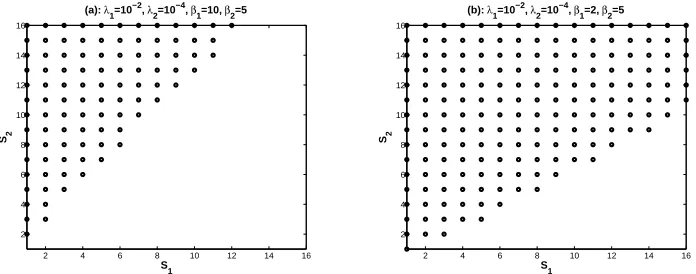
Fig. 1. Combinations of multiplexing gains for which ∂PMRCC

∂˜λ1 >0, whereα= 4,²1=²2= 0.1,P1= 50W, andP2= 1W.

C. Does Densification Always Improve the Coverage Probability?

We investigate the impact of densification on the coverage probability. We are interested in combinations of system parameters for which the coverage probability is increased by increasing the density of the BS in a given tier, namely tier 1: ∂P

MRC

C

∂λ˜1 > 0. For brevity, we set K = 2,

and λ˜1 = λ1(P1/S1)αˇ, λ˜2 = λ2(P2/S2)αˇ, Aji = µ

Γ(αˇ

Si+Sj)

Γ(Sj)

¶_Si

. In this case, it can be shown that for ∂P

MRC

C

∂˜λ1 > 0, it is necessary to have ˜

λ2 ˜

λ1(A21 −BA22) < A12B − A11, where B =

r³

(1−²2 1)β2S2 (1−²2

2)β1S1

´_αˇ

(Θ(β1,²1,S1))S1A21

(Θ(β2,²2,S2))S2A12. Fig. 1 shows various combinations of the multiplexing gains

that guarantee ˜λ2 ˜

λ1(A21−BA22)< A12B−A11. In general, for densification of tier 1 to be effective

in improving coverage performance, we need S2 > S1. In fact, as decoding S2 data streams is

more unlikely than S1 data streams, densification of tier 1 allows UEs to be more frequently

be associated with tier 1, thus improving the coverage probability. Moreover, by increasing β1,

we get a smaller number of multiplexing gain combinations, (S1, S2), in which densification

improves the coverage probability.

D. Coverage Performance of Relevant MIMO Communications Scenarios

Although Proposition 1 considers an open-loop tranceiver, one can utilize Proposition 1 to evaluate the coverage probability for various closed-loop scenarios, such as SISO (N_it =Nr = 1,

∀i) [6], MISO-SDMA (Nr = 1) [12, 28], Limited-feedback MISO-SDMA [28], and SIMO (Si =

1, ∀i). This is simply because the corresponding post-processing SIRs in the aforementioned closed loop techniques are often a function of the obtained SIR in (3).

For Peer Review

Assuming perfect CSI, immediate extensions of Proposition 1 are for zero-forcing beamform-ing (ZFBF) at the receiver, and orthogonal space-time block codes (OSTBC). Such extensions can be done after making proper adjustments to the number of DoFs in the desired and interfering signals through the general framework proposed in [32].

E. Selecting the Tranceiver Technique

We compare two prevalent open-loop techniques: ZFBF and MRC. Here we assume a perfect CSIR, i.e., ²i = 0 ∀i. We then set ΘZF(Si)=∆

Nr_−Si P

mi=0 Γ(αˇ

Si+mi)

Γ(αˇ

Si)Γ(1+mi)

. The coverage probability of the system with ZFBF was derived in [34] as:

PZF

C ≤

π

˜

C(α)

X

i∈K

λi

³

Pi

S2

iβi ´αˇ

(ΘZF_(S i))Si

P

j∈Kλj

³

Pj

Sj

´αˇµ_Γ(αˇ

Si+Sj)

Γ(Sj)

¶Si. (10)

This is consistent with Proposition 1, as P_CZF in (10) can also be obtained using the bound on

PMRC

C in Proposition 1, simply by substituting Θ(βi,0, Si) in (5) with ΘZF(Si).

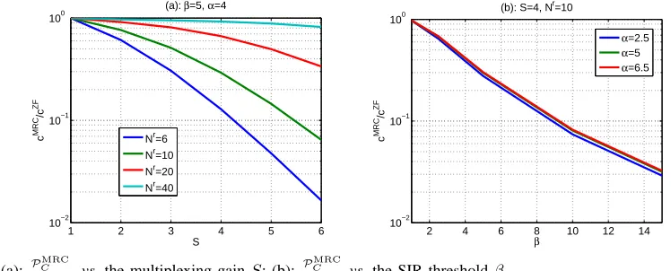
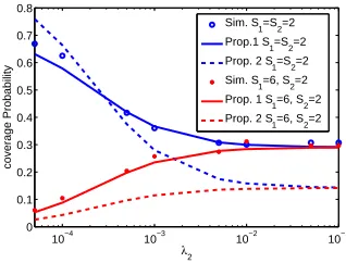
Using (10) and Proposition 1, we can now inspect whether ZFBF outperforms MRC. For clarity, we set K = 1. It is then straightforward to confirm that P_CZF > P_CMRC if ΘZF(Si) >

Θ(βi,0, Si). Fig. 2 shows that, in general, ZFBF yields a higher coverage probability than MRC.

This is mainly because the MRC receivers suffer from inter-stream interference. Furthermore, as shown in Fig. 2.a, by increasing the multiplexing gain, ZFBF becomes even more efficient than MRC. For a larger Nr, the superiority of ZFBF over MRC is shown to be reduced because the MRC receivers can harness diversity more effectively than ZFBF. Noticing that the ZFBF receiver complexity of a large arrays can be very high (because of the required matrix inversion operation), MRC provides room for compromising coverage performance (in fact, slightly for larger arrays) over computational complexity. Such aspects can be exploited in the design of HetNets. For instance, it is plausible to adaptively select either ZFBF or MRC in order to keep the prescribed coverage performance intact, while minimizing the complexity and energy consumption of the signal processing modules at the receivers.

Fig. 2.b also indicates that for a larger SIR threshold, β, ZFBF significantly outperforms MRC, while for small to moderate values of β, ZFBF is only slightly better than MRC. This observation suggests that for low-rate scenarios (e.g., for the cell-edge UEs) one can trade off

For Peer Review

1 2 3 4 5 6

10−2 10−1 100

c

MRC

/c

ZF

S (a): β=5, α=4

Nr=6 Nr=10 Nr=20 Nr=40

2 4 6 8 10 12 14 10−2

10−1 100

c

MRC

/c

ZF

β

(b): S=4, Nr=10

α=2.5

α=5

α=6.5

Fig. 2. (a): P

MRC

C

PZF

C , vs. the multiplexing gain

S; (b): P

MRC

C

PZF

C vs. the SIR threshold

β.

a slightly higher performance for a significantly lower computational complexity. Fig. 2 further indicates that the relative performance of ZFBF and MRC is not related to the path-loss exponent.

IV. CROSS-STREAMSIR CORRELATION

As it is also shown in (7), for a given MIMO receiver, the SIR values across streams are statistically correlated mainly because of the correlated interference among antennas due to the common locations of interferers. More specifically, the interference originated from near-by BSs may cause a high level of interference simultaneously to all of the data streams transmitted to a typical UE. As shown in the proof of Proposition 1, the cross-stream SIR correlation renders analytical complexities. In this section, we characterize the aforementioned correlation and analyze its impact on the system coverage performance.

A. SIR Correlation Coefficient

In a link, the coverage probability is related to the joint SIRs’ CDF of the streams. Here we focus on the SIR correlation instead of the ICI correlation. To quantify the SIR correlation, the Pearson correlation coefficients is used:

ρMRCxi (li, l 0

i) =

EhSIRMRC_xi,liSIRMRC_xi,l0 i

i

−SIRMRC_xi,li SIRMRC_xi,l0 i r

Var¡SIRMRC_xi,li¢Var

³

SIRMRC_xi,l0 i

´ =

EhSIRMRC_xi,li SIRMRC_xi,l0 i

i

−(SIRMRC_xi,li)2

Var¡SIRMRCxi,li

¢ , (11)

where E[.] is the expectation operator, SIRMRC_xi,li is the average SIR value on data stream li, and

Var[.] is the variance operator. The focus in the related literature (e.g., [35, 48]) is often on

For Peer Review

0

0.005

0.01

0 0.005

0.010 0.2 0.4 0.6 0.8

λ2

S

1=S2=6, α=4,ε1=0.1

λ₁

correlation coefficient

Fig. 3. Correlation coefficient vs. λ1 and λ2, where

K= 2,Nr = 8,xi= 20,P1= 50W, andP2= 10W.

0 0.5

1

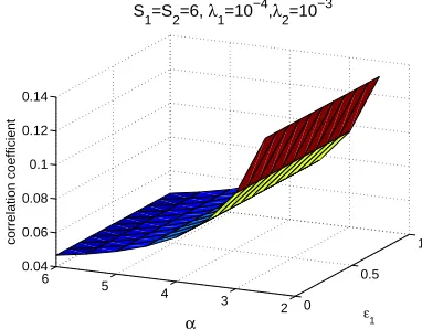
2 3 4 5 6 0.04 0.06 0.08 0.1 0.12 0.14

ε₁

S

1=S2=6, λ1=10 −4

,λ

2=10 −3

α

correlation coefficient

Fig. 4. Correlation coefficient vs.αand²1.

understanding of the interference correlation among antennas. In contrast, as [49] we here focus on the SIR correlation among data streams.

Proposition 2: For the typical UE receiving data from BS, xi, in a MIMO-MRC multiplexing

system, the correlation coefficient between data streams li and li0, ∀li, l0i, li 6=l0i is:

ρMRC xi (li, l

0

i) =

∞

R

0

∞

R

0

e −C˜(α)P

jλj( Pj

Sj) ˇαW j(t,τ)

1+(t+τ)Pi

Six−iα

− e−(tαˇ+ταˇ)Λ

(1+tPi

Six−iα)(1+τPiSix−iα)

³

1+tPi_Si²2

ix−iα

´³

1+τPi_Si²2

ix−iα

´³

(1+tPi_Six−α

i )(1+τPiSix−iα)

´_Si−2dtdτ

∞

R

0

∞

R

0



 N rN r+1e−(t+τ) ˇ αΛ

µ

1+(t+τ)Pi²2i Sixαi

¶³

1+(t+τ)Pi

Sixαi

´_Si−1 −

e−(tαˇ+ταˇ)Λ

³

1+ tPi

Sixαi ²

2

i

´µ

1+Pi²2i τ Sixαi

¶³

(1+ tPi

Sixαi)(1+ Piτ Sixαi )

´_Si−1



_dtdτ ,

(12)

where αˇ = 2/α, Λ,C˜(α)P

j

λj ³

Pj Sj

´_αˇ

Γ(ˇα+Sj)

Γ(Sj) , C˜(α),πΓ(1−αˇ), Γ(a),

∞ R

0

e−z_za−1_{dz, and}

Wj(t, τ), ∞ Z

0

∞ Z

0

(tg1+τ g2)αˇ

(g1g2)Sj−1 Γ2_(S

j)

e−(g1+g2)_dg

1dg2. (13)

Proof : See Appendix B. ¥

As shown in (12), the ICI affects the correlation coefficient mainly through Λ, where Λ is a function of BSs’ density, their transmission powers and multiplexing gains, and the corresponding path-loss exponent. It is further shown in (12) that the multiplexing gains and CSI estimation inaccuracy may affect the correlation by imposing self-interference.

Fig. 3 shows the impact ofλ1 andλ2 onρxiMRC(li, l0i). As it is seen for a sparse network, where

λ1 →0 and λ2 →0, the correlation coefficient is very close to 0. In other words, the network

behaves like an isolated link, where BSs are sparse in the coverage area. By increasing the

For Peer Review

density of BSs, however,ρMRC_xi (li, l0i) is proportionally increased such that in an extreme case of

high density of BSs where λ1 ≈0.01and/orλ2 ≈0.01, the SIRs of data streams become highly

correlated. In such a case, if a data stream, li, experiences outage due to a close-by interfering

BS, then other data streams l_i0 6=li will most likely experience the same.

Proposition 2 further shows that the imposed correlation due to the CSI estimation error seems negligible. This is because each individual data stream receives Si−1 inter-stream interference

which is much more powerful than the interference imposed by the CSI estimation error. Fig. 4 confirms this, indicating that the SIR correlation is not affected by change in the value of ²1.

The impact of path-loss exponent is also seen in Fig. 4. For a lower α, even a small number of moderately close interferers induce a substantial level of interference. This reduces the SIR for all data streams at the same time, thus causing a large correlation among data streams. For a higher value of α, the collective impact of the ICI received from the BSs located far from the receiver causes correlation, and hence unless the density of interferers is very high, the correlation is negligible.

One can therefore conclude that densification in multi-stream systems causes substantial SIR correlation among data streams through the ICI. This consequently affects the outage performance of the HetNet. Proposition 2, however, does not explicitly quantify the impact of the SIR correlation on the coverage performance.

B. Impact of SIR Correlation on the Coverage Performance

To analyze the impact of cross-stream SIR correlation on the coverage performance, here we introduce a multiplexing setting, namely full-correlation (FC) where the interference is fully correlated across all data streams in a link2. In other words, in the FC setting, the same level of ICI is received among all data streams in the communication link. Therefore, exchanging GMRC_xj,li with its average value, Sj, the ICI in the FC setting is IFC =

P

j∈K P

xj∈Φj/xi

Pjkxjk−α. Assuming

a typical UE is associated with BS xi, the corresponding post-processing SIR for stream li is SIRMRC_xi,li−FC=

Pi

Sikxik

−α_(1−²2 i)HxMRCi,li

Pi

Sikxikα ³

ˆ

HMRC xi,li +²

2 iH˜xMRCi,li

´

+IFC. (14)

2

In [36] a similar assumption made to quantify signal correlation of optimal-combining in SIMO ad hoc networks.

For Peer Review

Based on the adopted CA policy, the associated BS for a link is the one that its corresponding smallest SIR values SIRMRC_xi,li −FC across all data streams, is the maximum among all the BSs. Therefore, the typical UE is in coverage if

AMRC_all −FC=

½

∃i∈ K: max xi∈Φi

min li=1,...,Si

SIRMRC_xi,li−FC≥βi

¾

, (15)

is not empty. An upper-bound on the corresponding coverage probability,P_CMRC−FC, is given in the following proposition.

Proposition 3: In the FC setting, the coverage probability is upper-bounded as:

P_CMRC−FC≤ π ˜

C(α)PK j=1

λjPjαˇ

X

i∈K

λi

µ

Pi(1−²2i)

S2 iβi

¶αˇ

(Θ(βi, ²i, Si))Si. (16)

Proof : We prove the proposition by following the same line of argument as in the proof of

Proposition 1. In the FC setting, (7) is reduced to

PMRC−FC

C =

X

i∈K 2πλi

∞

Z

0

xiE{IFC_} Si Y

li=1

PnSIRMRC−FC xi,l ≥βi

¯

¯_IFCo_dx

i (17)

=X

i∈K 2πλi

∞ Z 0 xi Si Y

li=1 ∞

Z

0

L−1 ¯

F_HMRC

i

(ti)

³

1 + tiβi

1−²2

i ´Si−1

(1 + ti²2iβi

1−²2

i ) Y

j∈K

EΦj Y

xj∈Φj/xi e−ti

βiSixαi Pi(1−²2_i)Pjkxjk

−α dti

(a)

=X

i∈K 2πλi

∞ Z 0 xi ∞ Z 0 . . . ∞ Z 0

e−x

2

iC˜(α)

µ

βiSi Pi(1−²2_i)

¶_{α Kˇ} P

j=1 λjPjαˇ(

Si

P

li=1

t_li)αˇ YSi

li=1

L−F¯_H1MRC

i

(tli) ³

1 + tliβi

1−²2

i ´Si−1

(1 + tli²2iβi

1−²2

i ) dtli

(b)

= π

˜

C(α)PK j=1

λjPjαˇ

X

i∈K

λi

µ βiSi

Pi(1−²2i)

¶−αˇZ∞

0 . . . ∞ Z 0 ( Si X

li=1 tli)

−αˇ Si Y

li=1

L−1 ¯

F_HMRC

i

(tli) ³

1 + tliβi

1−²2

i ´Si−1

(1 +tli²2iβi

1−²2

i ) dtli

(c)

≤ π

˜

C(α)PK j=1

λjPjαˇ

X

i∈K

λi

µ βiSi2

Pi(1−²2i)

¶−αˇZ∞

0 . . . ∞ Z 0 Si Y

li=1

t−

ˇ

α Si

li L −1 ¯

F_HMRC

i

(tli) ³

1 + tliβi

1−²2

i ´Si−1

(1 +tli²2iβi

1−²2

i ) dtli

(d)

= π

˜

C(α)PK j=1

λjPjαˇ

X

i∈K

λi

µ βiSi2

Pi(1−²2i)

¶−α Sˇ Yi

li=1 ∞ Z 0 t− ˇ α Si

li L −1 ¯

F_HMRC

i

(tli) ³

1 + tliβi

1−²2

i ´Si−1

(1 + tli²2iβi

1−²2

i ) dtli

(e)

= π

˜

C(α)PK j=1

λjPjαˇ

X

i∈K

λi

µ βiSi2

Pi(1−²2i)

¶−αˇ

    ∞ Z 0 t− ˇ α Si

i L−_F¯1

H_iMRC

(ti)

³

1 + tiβi

1−²2

i ´Si−1

(1 +ti²2iβi

1−²2

For Peer Review

where in (a) we insert the Laplace transform of IFC and in (b) the integrals are reordered and we integrate the inner integral with respect to xi. In (c) arithmetic-geometric inequality is applied

followed by (d) and (e) where the fading gains,H_xi,liMRC, are i.i.d. Applying the result of Appendix A in (e), completes the proof. ¥ Comparing Propositions 1 and 3, we note that in general for the FC setting, the coverage probability has a more simplified form. On the other hand, the upper-bound of the coverage performance of a MIMO-MRC HetNet system is (almost) always higher than the same system assuming the FC setting. This is because by noting that for _Siαˇ ∈(0,1), there holds Γ(

ˇ

α Si+Sj)

Γ(Sj) .S ˇ

α Si j

[35]. Therefore, noticing that both (16) and (5) have the same nominator while the denominator of the former is larger than that of the latter, we obtain P_CMRC−FC . P_CMRC. Consequently, we can conclude that adding to the correlation among data streams of a communication link can reduce the coverage probability. Although this result is based on the derived upper-bounds on the coverage probabilities in (16) and (5), our simulation results in Section V confirm its credibility.

C. What If the Cross-Stream SIR Correlation Is Overlooked?

The above analysis shows that approximating a practical scenario based on the FC setting results in underestimation of the coverage probability. Another way to simplify the coverage analysis is to simply ignore the cross stream SIR correlation, i.e., statistically independent SIR values. We refer to this case as no-correlation (NC) setting. Starting from (7) and assuming the NC setting, the coverage probability in (7) is written as

P_CMRC−NC=X i∈K

2πλi

∞

Z

0

xi Si Y

li=1

EΦP

©

SIRMRCxi,li ≥βi ¯

¯_Φª_{dxi. (18)}

The coverage probability in (18) can then be written as:

PMRC−NC

C =

X

i∈K 2πλi

∞

Z

0

xi Si Y

li=1 ∞

Z

0

L−1 ¯

F_HMRC

i

(ti)

³

1 + tiβi

1−²2

i ´Si−1

(1 +ti²2iβi

1−²2

i ) Y

j∈K

EΦj Y

xj∈Φj/xi

EGMRC

xj ,lie

−t_li βiSixαi Pi(1−²2_i)

Pj GMRC_{xj ,li} Sjkxjkα

dti

(a)

= X

i∈K 2πλi

∞

Z

0

xi

∞

Z

0

. . .

∞

Z

0

e

−x2

iΛ

µ

βiSi Pi(1−²2_i)

¶_αˇ

(PSi

li=1 tαˇ

li)YSi

li=1

L−1 ¯

F_HMRC

i

(tli) ³

1 + tliβi

1−²2

i ´Si−1

(1 +tli²2iβi

1−²2

i ) dtli

= π Λ

X

i∈K

λi

µ βiSi

Pi(1−²2i)

¶−αˇZ∞

0

. . .

∞

Z

0

à _S i Y

li=1 tli

!−_{α S}ˇ

i Y

li=1

L−1 ¯

F_HMRC

i

(tli) ³

1 + tliβi

1−²2

i ´Si−1

(1 +tli²2iβi

1−²2

i ) dtli

For Peer Review

= π

Λ

X

i∈K

λi

µ βiSi2

Pi(1−²2i)

¶−α Sˇ Yi

li=1 ∞

Z

0

t−αˇ li L

−1 ¯

F_HMRC

i

(tli) ³

1 + tliβi

1−²2

i ´Si−1

(1 +tli²2iβi

1−²2

i ) dtli

(b)

= π

Λ

X

i∈K

λi

µ βiSi2

Pi(1−²2i)

¶−αˇ



 

∞

Z

0

t−αˇ i L−_F¯1

HMRC

i

(ti)

³

1 + tiβi

1−²2

i ´Si−1

(1 +ti²2iβi

1−²2

i ) dti



 

Si

,

where in (a) we insert the Laplace transform of the ICI and further notice the definition of Λ as in Proposition 2. Denoting the integral in (b) by Θ(˜ βi, ²i, Si) and following the same line of

argument as in Appendix A, we evaluate this integral as

˜

Θ(βi, ²i, Si), Nr₋₁

X

ri=0

ri X

qi=0

qi X

pi=0

(−1)qi−piβ2qi−pi

i

²−4qi+2pi

i (1−²2i)Si

¡

1−²2 i +βi

¢−qi−Si+1¡

1 +²2

i(βi−1)

¢−qi+pi−1

piB(Si−1, pi)(ri−qi)B(ˇα, ri−qi)

. (19)

Using this, (18) is then reduced to

P_CMRC−NC= π Λ

X

i∈K

λi

µ

Pi(1−²2i)

Siβi

¶αˇ_³

˜

Θ(βi, ²i, Si)

´Si

. (20)

Note that NC setting is in fact an extreme case and thus P_CMRC−NC is not practically achievable. This is simply because it does not comply with the max-SIR CA rule as in the NC setting, an independent set of interferers appears on each data stream. Therefore, there might be cases where the typical UE becomes associated with different BSs for different data streams. This, however, contradicts the reality of the MIMO signal model as presented in 1.

We further note that, as αˇ∈(0,1), by using Γ(ˇ_Γ(α+_SjSj₎) .S_jαˇ a lower-bound on P_CMRC−NC is

P_CMRC−NC& π P

i∈K

λi

³

Pi(1−²2i)

S2

iβi ´αˇ³

˜

Θ(βi, ²i, Si)

´Si

˜

C(α)PK j=1

λjPjαˇ

≥

πP

i∈K

λi

³

Pi(1−²2i)

S2

iβi ´αˇ

(Θ(βi, ²i, Si))Si

˜

C(α)PK j=1

λjPjαˇ

=P_CMRC−FC.

where the second inequality is because Θ(˜ βi, ²i, Si)≥ Θ(βi, ²i, Si). To confirm this, we notice

that the beta function is a decreasing function of its argument, and observing that by compar-ing Θ(˜ βi, ²i, Si) in (19) and Θ(βi, ²i, Si) in (6), we note that for a given positive number a,

˜

Θ(βi, ²i, Si)−Θ(βi, ²i, Si)∝ _B(ˇα,a1 ₎ − _B(α1ˇ

Si,a).

On the other hand, since _Siαˇ ∈(0,1), there holds Γ(

ˇ

α Si+Sj)

Γ(Sj) > S ˇ

α Si

j Γ(1 +Siαˇ) [35]. Applying this,

PMRC

C in (5) is further upper-bounded as PMRC

C ≤

πP

i∈K

λi

³

Pi(1−²2i)

S2

iβi ´αˇ³

Θ(βi, ²i, Si)Γ(1 +_Sαˇ_i)

´Si

˜

C(α)PK j=1

λjPjαˇ

≤

π P

i∈K

λi

³

Pi(1−²2i)

S2

iβi ´αˇ

(Θ(βi, ²i, Si)))Si

˜

C(α)PK j=1

λjPjαˇ

≤ P_CMRC−NC,

For Peer Review

where the last line is because Γ(1 +_Siαˇ)≤1for _Siαˇ ∈(0,1). Consequently, using the NC setting, the coverage probability is basically overestimated. This implies that the common approach that focuses on either isolated scenarios or non-isolated scenarios but with emphasis of the characterization of MIMO communications from the perspective of a data stream is essentially overestimation of the actual performance of the network.

V. SIMULATIONRESULTS

In this section, we use simulations to evaluate the performance of a MIMO-MRC HetNet setting and further examine the accuracy of the developed analysis. The simulated system is a 2-tier HetNet, i.e.,K = 2. The macro BS in the first tier has a high Tx power ofP1 = 50W. The

second tier consists of femto BSs with a low Tx power of P2 = 1W. The path-loss exponent is

α = 4, and the CSI estimation error ²i = 0.1 ∀i, N1t =N2t = 16. In a disk with radius 10,000

units, we randomly drop BSs of each tier according to the corresponding tier densities. We set

λU = 1 so all the BSs are assumed to be active. We apply Monte Carlo technique and analyze

40,000 snapshots of simulations. In each snapshot the MIMO channels are randomly generated. For the UEs, the corresponding SIR values are then calculated based on the MRC receiver.

A. Impact of Path-loss Exponent, CSI Estimation Error, and SIR Threshold

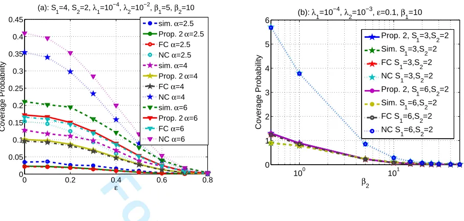
Fig. 5.a shows the coverage probability vs. the estimation error,²=²i,∀i, for several values of

the path-loss exponent, α. The bound obtained in Prop. 1 is shown to be close to the simulation result. Also, increasing the CSI inaccuracy is shown to reduce the coverage performance. This is because the interference on each data stream is increased due to the CSI inaccuracy. It is also seen in Fig. 5.a that increasing the path-loss exponent improves the outage performance. Noting that a largerα implies a smaller signal strength, the improved outage performance suggests that the ICI is the main limiting factor.

Fig. 5.a also shows that in contrast to the cases with a smaller path-loss exponent (e.g., outdoor communications), the coverage is not significantly affected by the CSI inaccuracy where the path-loss exponent is high (e.g., indoor communications). This suggests that a simpler transceiver

For Peer Review

0 0.2 0.4 0.6 0.8

0 0.05 0.1 0.15 0.2 0.25 0.3 0.35 0.4 0.45

ε

Coverage Probability

(a): S

1=4, S2=2, λ1=10 −4_{, λ}

2=10 −2_{, β}

1=5, β2=10

sim. α=2.5 Prop. 2 α=2.5 FC α=2.5 NC α=2.5 sim. α=4 Prop. 2 α=4 FC α=4 NC α=4 sim. α=6 Prop. 2 α=6 FC α=6 NC α=6

100 101

0 1 2 3 4 5 6

β

2

Coverage Probability

(b): λ

1=10 −4

, λ

2=10 −3

, ε=0.1, β

1=10

Prop. 2, S

1=3,S2=2

Sim. S

1=3,S2=2

FC S

1=3,S2=2

NC S

1=3,S2=2

Prop. 2, S

1=6,S2=2

Sim. S

1=6,S2=2

FC S

1=6,S2=2

NC S

1=6,S2=2

Fig. 5. (a): Coverage Probability vs. the CSI estimation error. (b): Coverage Probability vs.β2.

design or/and signaling protocol can be used without any significant compromise of the coverage probability. Fig. 5.b shows the coverage probability versus β2. The bound obtained in Prop. 1

is is shown to be sufficiently accurate even for small values of β2. It also shows that a higher

β2 results in a lower coverage performance.

B. Impact of Densificaiton and Multiplexing Gains

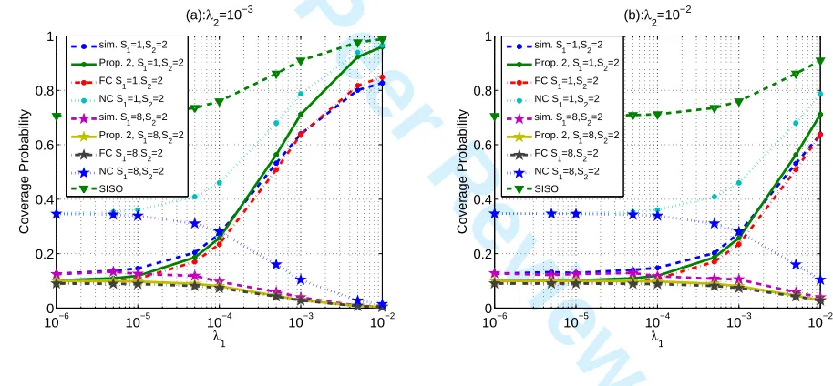
In Figs. 6 and 7 the coverage probability is given versus λ1. We consider 5 settings (Stg)

of multiplexing gains between two tiers, where Stg1, Stg2, Stg3, Stg4, and Stg5, respectively, refer to (S1 = 1, S2 = 1), (S1 = 4, S2 = 1), (S1 = 4, S2 = 2), (S1 = 1, S2 = 2), and (S1 = 8, S2 = 2). Fig. 6 shows the coverage performance for Stg1, Stg2, and Stg3. The results

of Stg1, Stg4, and Stg5 are plotted in Fig. 7. Both figures show the outage performance for

λ2 = 10−3, andλ2 = 10−2.

It is seen in Figs. 6 and 7 that the analytical result presented in Prop. 1 closely follows the simulation results. It is also observed that a single stream communications, Stg1, generally outperforms the other combinations of multiplexing gains, regardless of the density of the BSs in both tiers. For the single stream case, it is also seen that densification in tier1 always results in a higher improvement in the coverage probability. Nevertheless, comparison of Fig. 6.a with