arXiv:1702.08855v3 [hep-ph] 23 May 2017
Thermal Inflation with a Thermal Waterfall Scalar
Field Coupled to a Light Spectator Scalar Field
Konstantinos Dimopoulos
a, David H. Lyth
band Arron Rumsey
cConsortium for Fundamental Physics
Physics Department, Lancaster University
Lancaster, LA1 4YB, UK
akonst.dimopoulos@lancaster.ac.uk,b d.lyth@lancaster.ac.uk,ca.rumsey@lancaster.ac.uk
May 24, 2017
1
Introduction
Cosmological Inflation is the leading candidate for the solution of the three main problems of the stan-dard Big Bang cosmology: the horizon, flatness and relic problems. It also has the ability to seed the initial conditions required to explain the observed large-scale structure of the Universe [1]. In the simplest scenario, quantum fluctuations of a scalar field are converted to classical perturbations around the time of horizon exit, after which they become frozen. This gives rise to the primordial curvature perturbation,ζ, which grows under the influence of gravity to give rise to the large-scale structure in the Universe. The simple single-field inflationary sce-nario is favoured by current observations [2]. How-ever, given the richness and complexity of the theo-ries beyond the standard model, this simple picture seems unlikely.
Moving away from this simplest scenario, there has been much work done on generating the ob-served ζ in other scenarios, such as the curvaton [3–14], inhomogeneous reheating [5,10–13,15–20], “end of inflation” [9,20–26] (also see [27]) and in-homogeneous phase transition [28] (also see [29]).
One particular model of inflation is thermal in-flation [30–33], which is a brief period of inflation that could have occurred after a period of prior pri-mordial inflation. Thermal inflation lasts too little to solve the problems of the standard Big Bang cos-mology that motivate primordial inflation, but it may be rather useful to dilute any dangerous relics that are not dealt with by primordial inflation such as moduli fields or gravitinos. Another interesting byproduct of thermal inflation is changing the num-ber of e-folds before the end of primordial inflation, which correspond to the cosmological scales. This has an immediate effect on inflationary observables and can assist in inflation model building [34,35].
Thermal inflation occurs due to finite-temperature effects arising from a coupling between a so-called thermal waterfall scalar field φ and the thermal bath created from the partial or complete reheat-ing from primordial inflation. Thermal field theory gives a thermal contributiong2T2φ2to the effective
scalar potential, wheregis the coupling constant of the interaction betweenφand the thermal bath and
T is the bath’s temperature. This results in a ther-mal correction to the effective mass of g2T2. This
thermal mass can temporarily trap the thermal wa-terfall field on top of a false vacuum, resulting in inflation. However, as time goes by, the thermal mass of φ decreases such that a phase transition sendsφto its vacuum expectation value (VEV) and inflation is terminated.
Despite occurring much later than primordial inflation, thermal inflation may produce a substan-tial contribution to the curvature perturbation. This
is how. The mass of a given scalar field may de-pend on the expectation value of another scalar field. [9,13,16–19,21–24,28,29]. More specifically, the mass of a thermal waterfall field φ that is re-sponsible for a bout of thermal inflation could be dependent on another scalar field ψ. We will call this ψ a spectator field, because it needs not af-fect the dynamics of the Universe at any time. If
ψ is light during primordial inflation, its quantum fluctuations are converted to almost scale-invariant classical field perturbations at around the time of horizon exit. If ψ remains light all the way up to the end of thermal inflation, then thermal infla-tion will end at different times in different parts of the Universe, because the value of the spectator field determines the mass of the thermal waterfall field φ, which in turn determines the end of ther-mal inflation. This is the “end of inflation” mecha-nism [21] and it can generate a contribution to the primordial curvature perturbation ζ. The motiva-tion of this work is to explore this scenario to see if it can produce the dominant contribution to the primordial curvature perturbation with characteris-tic observational signatures, in which the inflaton’s contribution to the perturbation can be ignored.1
As such, inflation model building is liberated from the requirements to generateζ, which substantially reduces fine-tuning and renders viable many other-wise observationally excluded inflation models [37]. It should be noted that this scenario is very sim-ilar to that in Ref. [20]. However, in that paper the authors use a modulated coupling constant rather than a modulated mass. Also, the treatment that has been given to the work in this paper is much more comprehensive. One example of this is in the consideration of the effect that the thermal fluctua-tion of the thermal waterfall field has on the model (see Section4.2.6). Another example is the require-ment that the thermal waterfall field is thermalized (see Section4.2.7). Also, there is no consideration given in Ref. [20] to requiring a fast transition from thermal inflation to thermal waterfall field oscilla-tion (see Secoscilla-tion4.2.10), as detailed in Ref. [24], as this paper appeared after Ref. [20].
This paper is structured as follows. In Section2
we introduce our new model. In Section3 we give expressions for key observational quantities that are predicted by the model. In Section4we explore the “end of inflation” scenario and obtain in detail a multitude of constraints for our model parameters. We conclude in Section5.
Throughout this work, natural units are used where c=~=kB= 1 and Newton’s gravitational constant is 8πG=M−2
P , withMP= 2.436×10¹⁸GeV being the reduced Planck Mass.
1
This paper is based on the original research that was
conducted as part of the thesis [36]. This research has not
2
A new Thermal Inflation model
The potential that we consider in our model is
V(φ, ψ, T) =V0+
g2T2−12m20+h 2 ψ2α
M2α−2
P
φ2
+λφ
2n+4
M2n P
+1 2m
2
ψψ2, (2.1)
where φ is the thermal waterfall scalar field, ψ is a light spectator scalar field, T is the tempera-ture of the thermal bath, g, h and λ are dimen-sionless coupling constants, α ≥ 1 and n ≥1 are integers, V0 is a density scale (corresponding to
the scale of thermal inflation) and the −m2 0 and
m2
ψ are soft mass-squared terms coming form su-persymmetry (SUSY) breaking. A φ4 term is not
featured because the thermal waterfall field is a flaton, whose potential is stabilised by the higher-order non-renormalisable term [30,31].2 The
non-renormalisable terms in Eq. (2.1) are the dominant terms in series overαandn. One would expect the lowest order to be dominant. Indeed, we find that parameter space exists only ifα=n= 1. Thus, we chose these values in this paper.3 With this choice,
the potential in Eq. (2.1) becomes
V(φ, ψ, T) =V0+
g2T2
−12m2 0+h
2ψ2
φ2
+λ φ
6
M2
P +1
2m
2
ψψ
2
, (2.2)
We make the following definition
m2
≡m2
0−2h2ψ2. (2.3)
The variation ofm(ψ) is
δm=−2h
2ψ
m δψ . (2.4)
We only consider the case where the mass of
φ is coupled to one field. Were the mass coupled to several similar fields, the results would be just multiplied by the number of fields. If the multiple fields are different, then there will be only a small number that dominate the contribution to the mass perturbation. Therefore we consider only one for simplicity.
Using Eq. (2.3), the potential becomes
V(φ, ψ, T) =V0+
g2T2−12m2
φ2
+λ φ
6
M2
P +1
2m
2
ψψ2. (2.5)
This potential is shown in Fig.1. It would appear
2
Note here, that mild tuning (A <1 TeV) is needed for
the quartic term due to the SUSY A-term to be ignored.
3
For a full study over all possible values ofαandnsee
[36].
[image:3.595.319.506.74.237.2]Arbitrary Units
Fig. 1: The potential given by Eq. (2.5).
from the potential that domain walls will be pro-duced, due to the fact that in some parts of the Universe φ will roll down to +hφi while in others parts it will roll down to − hφi. However, being a flaton field (i.e. a flat direction in SUSY) φ is a complex field, whose potential contains only one continuous vacuum expectation value (VEV).4
The zero temperature potential is
V(φ, ψ,0) =V0−
1 2m
2φ2+λ φ6
M2
P +1
2m
2
ψψ2. (2.6)
Hence, the VEV is
hφi ∼
mM
P √
λ
1/2
. (2.7)
V0 is obtained by requiringV(hφi) = 0 along the
ψ= 0 direction. We find
V0∼
m3 0MP
√
λ . (2.8)
Now, we use the Friedmann equation
M2
PHTI2 ∼V0, (2.9)
to obtain the Hubble parameter during thermal in-flation as
HTI∼
m3 0
√
λ MP
1/2
. (2.10)
Within this thermal inflation model there are two cases regarding the decay rate of the inflaton field Γϕ, with ϕ being the inflaton, i.e. the field driving primordial inflation prior to thermal infla-tion. One is the case when Γϕ &HTI, i.e. that
4
A complex φmay result in the copious appearance of
cosmic strings after the end of thermal inflation. However,
as their energy scale is very low (it isV0), they will not have
reheating from primordial inflation occurs before or around the time of the start of thermal inflation. Alternatively, there is the case when Γϕ≪HTI, i.e.
that reheating from primordial inflation occurs at some time after the end of thermal inflation.
In the case of Γϕ&HTI, thermal inflation begins
at a temperature
T1∼V01/4 (2.11)
T1corresponds to the temperature when the
poten-tial energy density becomes comparable with the energy density of the thermal bath, for which the density isργ∼T4.
In the case of Γϕ≪HTI, thermal inflation
be-gins at a temperature5
T1∼ MP2HTIΓϕ
1/4
(2.12)
Initially, for T ≥T1, the thermal waterfall field is
driven to zeroφ→0 as the thermally induced mass in Eq. (2.5) is dominant. This continues even if
T < T1 as long as the mass squared of φ remains
positive. When the tachyonic mass term of the thermal waterfall field becomes equal to the thermally-induced mass term (cf. Eq. (2.5)) a phase transition sends the field towards its non-zero true VEV and thermal inflation ends [30].
In both of the above cases, thermal inflation ends at a temperature
T2=
m
√
2g. (2.13)
In the following, we only consider the case where Γϕ≪HTI, in that reheating from primordial
infla-tion occurs at some time after the end of thermal inflation, as this scenario was found to yield more parameter space than the case where Γϕ&HTI.
3
φ
Decay Rate, Spectral
In-dex and Tensor Fraction
3.1
φ
Decay Rate
The decay rate ofφis given by
Γ∼max
g2m , m 3
M2
P
(3.1)
The first expression is for decay into the thermal bath via direct interactions and the second is for gravitational decay. We will only consider the case in which the direct decay is the dominant channel (g is not taken to be very small). This is the case whenm≪gMP. Therefore we have just Γ∼g2m.
5
Before primordial reheating, the temperature is
T ∼ M2
PHΓϕ
1/4
[38].
3.2
Spectral Index and its running
Thermal Inflation has the effect of changing the number of e-folds before the end of primordial infla-tion at which cosmological scales exit the horizon. This affects the value of the spectral indexnsof the curvature perturbationζ(see for example [34,35]). We assume ζ is generated due to the pertur-bations of the spectator scalar field. Then, in the case of slow-roll inflation, the spectral index is given by [1]
ns≃1−2ǫ+ 2ηψ. (3.2)
whereǫandηψare slow-roll parameters, defined as
ǫ≡ M
2
P 2
V′
(ϕ)
V(ϕ)
2
and ηψ ≡ 1 3H2
∂2V
∂ψ2,
(3.3) whereV′
(ϕ) is the derivative of the inflaton poten-tial with respect to the inflaton field ϕ. ǫ andηψ are to be evaluated at the point where cosmological scales exit the horizon during primordial inflation. Regarding the various scalar fields involved in this model, the reason whyǫdepends only onϕis because this slow-roll parameter captures the infla-tionary dynamics of primordial inflation, which is governed only by ϕ in our model (we are assum-ing that both ψ and φ have settled to a constant value (Sections4.2.5and4.2.8respectively) by the time cosmological scales exit the horizon during pri-mordial inflation). In a similar fashion, the reason why the slow-roll parameterηψ depends only on ψ is because this parameter captures the dependence on the spectral index of the field(s) whose pertur-bations contribute to the observed primordial cur-vature perturbationζ. In our case, this is only the spectator fieldψ.
The definition of the running of the spectral in-dex is [1]
n′
s≡ dns d lnk ≃ −
dns
dN , (3.4)
the second equation coming from d lnk= d ln (aH)≃
Hdt≡ −dN, where k=aH. From Eq. (3.2), we have
n′
s≃2 dǫ
dN −2
dηψ dN ≃2ǫ
d lnǫ
dN −2
dηψ
dN . (3.5)
Now, we have [1]
d lnǫ
dN ≃ −4ǫ+ 2η , (3.6)
whereη is a slow-roll parameter given by
η≡M2
P
V′′
(ϕ)
V(ϕ) . (3.7)
Also,
dηψ dN =−
1 3H4
d(H2)
dN ∂2V
∂ψ2 =−2ηψ
d lnH
where we used that V(ψ) does not depend on N, as we are assuming that both ψ and φ have set-tled to a constant value (Sections 4.2.5 and 4.2.8
respectively) by the time cosmological scales exit the horizon during primordial inflation.
Since [1],
d lnH
dN ≃ǫ , (3.9)
we have
dηψ
dN ≃ −2ǫηψ. (3.10)
Therefore, the final result for the running of the spectral index is
n′
s≃ −8ǫ
2
+ 4ǫη+ 4ǫηψ. (3.11)
From now on we assume that H has the con-stant valueH∗ by the time cosmological scales exit
the horizon up until the end of primordial inflation. In order to obtainǫ andη, we require the value of
N∗, the number of e-folds before the end of
pri-mordial inflation at which cosmological scales exit the horizon. We consider the period between when the pivot scale,k0≡0.002 Mpc−1, exits the horizon
during primordial inflation and when it reenters the horizon long after the end of thermal inflation. We have
R∗=H −1
∗ and (k0/apiv)
−1=H−1
piv, (3.12)
where R∗ is a length scale when the pivot scale
exits the horizon during primordial inflation and the subscript ‘piv’ denotes the time when this scale re-enters the horizon, withabeing the scale factor of the Universe. Therefore
H−1
∗ =
a∗
apiv
H−1
piv. (3.13)
Using the above, we now can calculateN∗.
Since Γϕ≪HTI, we have
eN∗=H∗ k
T
start,TI
Tend,inf
8/3T
reh,TI
Tend,TI
8/3T
pive−NTI
Treh,TI
(3.14)
whereNTIis the number of e-folds of thermal
infla-tion and the subscripts denote the following: ‘end,inf’ is at the end of primordial inflation, ‘start,TI’ is at the start of thermal inflation, ‘end,TI’ is at the end of thermal inflation and ‘reh,TI’ is at ther-mal inflation reheating. For the period between the end of primordial/thermal inflation and primor-dial/thermal inflation reheating, a∝T−8/3.6 For
all other times,a∝T−1.
We need to calculateTpiv. We consider the
pe-riod between when the pivot scale reenters the hori-zon and the present. Throughout this period the
6
During this time,T∼ M2
PHΓϕ
1/4
[38]. AsH∝t−1
we haveT∝t−1/4
. During the field oscillations, the Universe
is matter dominated and so we havea∝t2/3
. Putting this
all together we findT ∝t−1/4
∝a−3/8
.
Universe is matter-dominated (ignoring dark en-ergy). Therefore we haveρ∝a−3
∝T3. Using the
Friedmann equation, 3M2
PH2∝T3 we have
H2 piv
H2 0
=T
3 piv
T3 0
⇒ Tpiv= 9.830×10
−13GeV (3.15)
where ‘0’ denotes the values at present. Using this, we obtainN∗ as
N∗≈ln
3.2×1037GeV−1
H∗
0.002
!
+2 3ln
Γ
H∗
+1 4ln
10π2 9.8
×10−13GeV4
9M2
PΓ2
!
−NTI,
(3.16)
where we have usedg∗≈102as the number of spin
states (effective relativistic degrees of freedom) of the particles in the thermal bath, at the time of both primordial inflation reheating and thermal in-flation reheating.7
3.3
Tensor Fraction
r
The definition of the tensor fraction isr≡ Ph/Pζ [1], where Ph and Pζ are the spectra of the pri-mordial tensor and curvature perturbations respec-tively. The spectrumPh is given by
Ph(k) = 8
M2
P
H
k 2π
2
(3.17)
for a given wavenumberk. Using this, together with
ρ∗= 3MP2H∗2, given that we are saying Hk =H∗
for our current case, as well as the observed value Pζ(k0) = 2.142×10⁻⁹, we obtain
r= ρ
1/4
∗
3.25×1016GeV
!4
(3.18)
4
End-of-Inflation Mechanism
In this section we investigate the “end of inflation” mechanism. We aim to obtain a number of con-straints on the model parameters and the initial conditions for the fields. Considering these con-straints, we intend to determine the available pa-rameter space. In this papa-rameter space we will cal-culate distinct observational signatures that may test this scenario in the near future.8
7
Eq. (3.16) is only valid as long asNTI>0. Otherwise
N∗is independent of Γ.
8
We also investigated a modulated decay rate scenario, but found that there was no parameter space available. For
4.1
Generating
ζ
Asφis coupled toψ, the “end of inflation” mecha-nism will generate a contribution to the primordial curvature perturbationζ [21]. We use theδN for-malism to calculate this contribution as
ζ=δNTI=
dNTI
dm δm+
1 2!
d2N TI
dm2 δm 2+1
3! d3N
TI
dm3 δm 3+
· · · .
(4.1) The number of e-folds between the start and end of thermal inflation is given by
NTI= ln
a2
a1
= ln
T1
T2
, (4.2)
wherea1=astart,TIanda2=aend,TI.
Substituting T1 and T2, Eqs. (2.12) and (2.13)
respectively, into Eq. (4.2) gives
NTI≃ln
"√
2g M2
PHTIΓϕ
1/4
m
#
≃ 18ln g
8
√
λ M3
PΓ
2
ϕ
m5
!
, (4.3)
where we used Eq. (2.10)
Therefore theδN formalism to third order gives
ζ=δNTI=−
5 8
δm
m +
5 16
δm2
m2 −
5 24
δm3
m3 . (4.4)
By substituting our mass definition and its differ-ential, Eqs. (2.3) and (2.4), into Eq. (4.4) we ob-tain the power spectrum of the primordial curva-ture perturbation,9 which to first order is
p
Pζ = 5 8π
h2H
∗ψ
m2 . (4.5)
A required condition for the perturbative ex-pansion in Eq. (4.4) to be suitable is that each term is much smaller than the preceding one. This re-quirement gives
h2H
∗ψ
m2 ≪1, (4.6)
which is readily satisfied asp
Pζ ≪1.
4.2
Constraining the Parameters
In this section we produce a number of constraints for the model parameters and we describe the ra-tionale behind them.
9
It must be noted that although there will be
perturba-tions inψthat are generated during thermal inflation that
will become classical due to inflation, the scales to which these correspond are much smaller than cosmological scales, as thermal inflation lasts for only about 10-15 e-folds. There-fore we do not consider them here.
4.2.1 Primordial Inflation Energy Scale
We want the energy scale of primordial inflation to be V1/4.1014GeV so that the inflaton
contri-bution to the curvature perturbation is negligible. Therefore, from the Friedmann equation we require
H∗.10
10GeV (4.7)
4.2.2 Thermal Inflation Dynamics
We will consider only the case in which the infla-tionary trajectory is 1-dimensional, in that only the
φfield is involved in determining the trajectory of thermal inflation in field space. We do this only to work with the simplest scenario for the trajectory. It is not a requirement on the model itself. In or-der that theψfield does not affect the inflationary trajectory during thermal inflation, we require from ourmmass definition, Eq. (2.3), that
m0&hψ . (4.8)
Therefore we havem≃m0.
From our potential, at the onset of thermal in-flation, Eq. (2.2), Eq. (4.8) gives
m20<2g 2
T12. (4.9)
For Γϕ≪HTI, substitutingT1 from Eq. (2.12) into
Eq. (4.9) gives
m0<
g4Γ
ϕ
2MP3
√
λ
1/5
. (4.10)
4.2.3 Lack of Observation ofφ Particles
Given that we have not observed any φ particles, the constraint on the present value of the effective mass ofφ is mφ,now&1 TeV. From our potential,
Eq. (2.2), we havem2
φ,now∼ −m 2
0+ 30λhφi 4
/M2
P. Substituting the VEV of φ, Eq. (2.7), into here gives mφ,now∼m0 for all reasonable values of n.
Therefore, we require
m0&1 TeV. (4.11)
4.2.4 Light auxiliary field ψ
In order thatψacquires classical perturbations dur-ing primordial inflation, we require ψ to be light during this time, i.e. |mψ,eff| ≪H∗, where we are
using notation such that |mψ,eff| ≡
r
m
2
ψ,eff
. We
have
m2
ψ,eff=m2ψ+ 2h2φ2. (4.12) Therefore we need
mψ< H∗ and hφ∗< H∗, (4.13)
where φ∗ andψ∗ are the values ofφ andψ during
We require thatψremains atψ∗, the value
dur-ing primordial inflation, all the way up to the end of thermal inflation. The reason for this is that if ψ started to move, then its perturbation would decrease. This is because ψ unfreezes when the Hubble parameter becomes less than ψ’s mass, i.e.
H < mψ. In this case, the perturbation of ψ also unfreezes, because it has the same mass asψ. The density of the oscillatingψ field decreases as mat-ter, som2
ψψ2∝a
−3⇒ψ∝a−3/2. The same is true
for the perturbation, i.e. δψ∝a−3/2. So the whole
effect of perturbing the end of thermal inflation is diminished. Requiring thatψ is light at all times up until the end of thermal inflation is sufficient to ensure that the field and its perturbation remain at
ψ∗ andδψ∗respectively. Therefore we require
mψ< HTI (4.14)
which is of course stronger than just mψ≪H∗ in
Eq. (4.13).
Similarly toφ, given that we have not observed any ψparticles, the most liberal constraint on the present value of the effective mass ofψis
mψ,now&1 TeV (4.15)
4.2.5 The Field Valueψ∗
Substituting the observed spectrum valuePζ(k0) =
2.142×10⁻⁹into Eq. (4.5) gives the constraint
ψ∗∼10 −4 m
2 0
h2H
∗
. (4.16)
Substituting Eq. (4.16) into Eq. (4.8), regarding the dynamics of thermal inflation, gives
h&10−4m0
H∗
. (4.17)
Rearranging this form0 gives the constraint
m0.104hH∗. (4.18)
We require the field value ofψto be much larger than its perturbation, i.e. ψ∗ ≫ δψ∗, so that the
perturbative approach is valid. Therefore, with
δψ∗∼H∗, we obtain
ψ∗≫H∗ and
δψ∗
ψ∗
≪1. (4.19)
Combining the frozen valueψ∗, Eq. (4.16), with the
above gives
m0>102hH∗. (4.20)
Thus, we find the following range
102< m0
hH∗
<104. (4.21)
4.2.6 Thermal Fluctuation ofφ
The effective mass of φ at the end of primordial inflation is
m2
φ,end,inf∼g 2T2
end,inf−m 2 0∼g
2T2
end,inf, (4.22)
sincegTend,inf≫m0[36].
As we are dealing with the thermal fluctuation ofφaboutφ= 0, we havehδφiT=hφiT. The ther-mal fluctuation ofφis
q
hφ2iT ∼T (4.23)
and we require [36]
g <1, (4.24)
becauseg is a perturbative coupling.
In order to keepmψ,efflight, we require (cf.Section4.2.4),
hT1< HTI. (4.25)
During the time between the end of primordial in-flation and primordial inin-flation reheating,T∝a−3/8
andH∝a−3/2. Therefore, if Eq. (4.25) is satisfied,
then equivalent constraints for higherT andH are guaranteed to be satisfied as well.
Considering Γϕ≪HTI, by substituting Eqs. (2.10),
(2.12) and (4.16) into Eq. (4.25) we obtain the con-straint
h <
λ−3/2 m 9 0
M7
PΓ2ϕ
1/8
(4.26)
Rearranging this form0 gives
m0>
λ3/2h8M7
PΓ2ϕ
1/9
. (4.27)
4.2.7 Thermalization ofφ
In order thatφinteracts with the thermal bath and therefore that we actually have the g2T2φ2 term
in our potential, Eq. (2.2), we require Γtherm> H,
where Γtherm is the thermalization rate ofφ, which
is given by
Γtherm=nhσvi ∼σ T3, (4.28)
where n∼T3 is the number density of particles in
the thermal bath, σis the scattering cross-section for the interaction ofφand the particles in the ther-mal bath,vis the relative velocity between aφ par-ticle and a thermal bath parpar-ticle (which in our case is≈c= 1) and h i denotes a thermal average. The scattering cross-sectionσis given by
σ∼ g
4
E2 cm
, (4.29)
where Ecm is the centre-of-mass energy, which is
Ecm∼T. Substituting this into Eq. (4.29) gives
σ∼ g
4
This scattering cross-section is the total cross-section for all types of scattering (e.g. elastic) that can take place between φ and the particles in the thermal bath.10 The thermalization rate now becomes
Γtherm∼g4T . (4.31)
As before, during the time between the end of primordial inflation and primordial inflation reheat-ing, T ∝a−3/8 and H ∝a−3/2. Therefore, if the
constraint Γtherm> His satisfied at the time of the
end of primordial inflation, then it is satisfied all the way up to the start of thermal inflation. Thus, we have the constraint
Γtherm&H∗. (4.32)
Taking Eq. (4.31) withT∼ M2
PH∗Γϕ
1/4
gives
Γϕ&
H3
∗
g16M2
P
. (4.33)
We also require Γtherm> Hto be satisfied
through-out the whole of thermal inflation. Therefore, we have the constraint
g4T
2> HTI. (4.34)
Substituting HTI and T2, Eqs. (2.10) and (2.13)
into the above gives
m0< g6
√
λ MP . (4.35)
4.2.8 The Field Valueφ∗
We consider two possible cases for the value of the thermal waterfall field φ during primordial infla-tion, withmφ,infbeing the effective mass ofφ
dur-ing primordial inflation:
A) φ heavy, i.e. |mφ,inf| ≫ H∗, in which φrolls
down to its VEV.
B) φlight, i.e. |mφ,inf| ≪H∗, in whichφis at the
Bunch-Davies value (to be explained below).
Case A
Substituting hφi, Eq. (2.7), into Eq. (4.13) gives
h < λ1/4 H∗
√
m0MP
. (4.36)
Rearranging this form0 gives
m0<
√
λ h2
H2
∗
MP
. (4.37)
10
For a complete Field Theory derivation of the elastic
scattering cross-section betweenφand the thermal bath, see
[36].
Case B
We considerφto be at the Bunch-Davies value
φBD∼
M
PH∗2
√
λ
1/3
, (4.38)
corresponding to the Bunch-Davies vacuum [39], which is the unique quantum state that corresponds to the vacuum, i.e. no particle quanta, in the infi-nite past in conformal time in a de Sitter spacetime.
φBDis of this form asλφ6/MP2 ∼H∗4, this being
be-cause the probability of this Bunch-Davies state is proportional to the factore−V /H4
[40].
Substituting φBD, Eq. (4.38), into Eq. (4.13)
gives
h < λ1/6
H
∗
MP
1/3
. (4.39)
4.2.9 Energy Density ofφ
We require the energy density ofφto be subdomi-nant at all times, in order that it does not cause any inflation by itself. During the period between the end of primordial inflation and the start of thermal inflation, the energy density ofφis
ρφ∼g2T2φ2∼g2T4, (4.40)
the second equation coming from the thermal fluc-tuation φ ∼T. Therefore, considering the Fried-mann equation, we require
g T2
1 < MPHTI. (4.41)
During the time between the end of primordial in-flation and primordial inin-flation reheating,T∝a−3/8
andH∝a−3/2. Therefore, if Eq. (4.41) is satisfied,
then equivalent constraints for higherT andH are guaranteed to be satisfied as well.
Using that Γϕ≪HTI, by substitutingHTI and
T1, Eqs. (2.10) and (2.12) into Eq. (4.41) we obtain
m0>
h
g2Γϕ
2√
λ MP
i1/3
. (4.42)
φ∗ Case A
The energy density ofφduring primordial inflation is
ρφ,inf=
−1 2m
2 0+h
2ψ2
∗
hφi2+λhφi
6
M2
P
∼ −1 2m
2 0hφi
2
+λhφi
6
M2
P
, (4.43)
with the second equation coming from Eq. (4.8) re-garding the dynamics of thermal inflation. There-fore, with the energy density of the Universe being ∼M2
PH∗2, we require
m0hφi< MPH∗ and
√
λhφi3< M2
PH∗.
Substitutinghφi, Eq. (2.7), into the above gives the constraint
m0<
√
λ MPH∗2
1/3
. (4.45)
φ∗ Case B
The energy density ofφduring primordial inflation is
ρφ,inf=
−12m2 0+h2ψ2∗
φ2 BD+λ
φ6 BD
M2
P
∼ −12m2
0φ2BD+λ
φ6 BD
M2
P
, (4.46)
with the second equation coming from Eq. (4.8) re-garding the dynamics of thermal inflation. There-fore, with the energy density of the Universe being ∼M2
PH∗2, we require
m0φBD< MPH∗ and
√
λ φ3 BD < M
2
PH∗
(4.47) Substituting φBD, Eq. (4.38), into the above gives
m0<
√
λ M2
PH∗
1/3
. (4.48)
4.2.10 Transition from Thermal Inflation to Thermal Waterfall Field Oscillation
In order for the equations of theδN formalism that are derived within the context of the “end of infla-tion” mechanism to be valid, we require the tran-sition from thermal inflation to thermal waterfall field oscillation to be sufficiently fast [24]. More specifically, we require
∆t < δt1→2, (4.49)
where ∆t≡t2−t1 is the time taken for the
transi-tion to occur andδt1→2is the proper time between
a uniform energy density spacetime slice just before the transition att1and one just after the transition
at t2 when φ starts to oscillate around its VEV.
Qualitatively, we require the thickness of the tran-sition slice to be much smaller than its warping.
The primordial curvature perturbation that is generated by the “end of inflation” mechanism is
ζ=HTIδt1→2. (4.50)
Therefore, from Eq. (4.49) we require
ζ > HTI∆t . (4.51)
To calculateφ1 andφ2, the value of φat times
t1 andt2respectively, we use the fact that the
pro-cess is so rapid that it takes place in less than a Hubble time, so that the Universe expansion can be ignored. Then the equation of motion is
¨
φ+∂V
∂φ ≃0. (4.52)
At the end of thermal inflation,φis not centred on the origin, but has started to roll down the potential slightly. At this time, g2T2 is much smaller than
m2
0. Therefore we have
∂V ∂φ ≃ −m
2
0φ . (4.53)
So we have the equation of motion ¨φ≃m2
0φwhose
solution is
φ∝em0t
, (4.54)
where we are considering only the growing mode. Therefore we have
ln
φ
2
φ1
∼m0(t2−t1)∼m0∆t . (4.55)
We know thatφ1∼T ∼m0 and φ2∼ hφi.
There-fore we have
ln
"
1
√
λ MP
m0
1/2#
∼m0∆t . (4.56)
For all values of λ and m0, we have ∆t ≥m
−1 0 .
Therefore, from Eq. (4.51) we have
ζ > HTI m0
. (4.57)
Thus, given thatζ∼10−5, we require
HTI<10
−5m
0. (4.58)
We obtain an additional constraint by substitut-ing Eq. (4.58) into the requirement of mψ≪HTI,
Eq. (4.14). This gives
mψ<10−5m0. (4.59)
A further constraint is obtained by substituting
HT I, Eq. (2.10), into Eq. (4.58). We obtain
m0<10−10
√
λ MP . (4.60)
4.2.11 Energy Density of the Oscillatingψ
As ψ has acquired perturbations from primordial inflation, we require it not to dominate the energy density of the Universe after the end of thermal inflation when it is oscillating, at which time the effective mass ofψ is increased significantly due to the coupling of ψ to φ. This is so as not to allow
The energy density of the oscillatingψfield after the end of thermal inflation is
ρψ,osc=h2ψ2φ2+
1 2m
2
ψψ2∼h2ψ∗2hφi
2
+1 2m
2
ψψ∗2.
(4.61) For simplicity, we assume thatψdecays around the same time asφ, i.e. thatH does not change much between the time whenφdecays and the time when
ψdecays. Therefore, the energy density of the Uni-verse at the time when ψ decays is ∼M2
PΓ2. We therefore require
ρψ,osc∼h2ψ∗2hφi
2
+1 2m
2
ψψ∗2< M
2
PΓ2, (4.62)
which means
mψ< MPΓ
ψ∗
and hhφiψ∗< MPΓ. (4.63)
Substituting hφi, Γ and ψ∗, Eqs. (2.7) and (4.16)
and using that Γ∼g2m(withg <1) into Eq. (4.63)
gives the constraints
h >10−4
g−2
λ−1/4 MP
H∗
m
0
MP
3/2
and
mψ<(102gh)2
MPH∗
m0
. (4.64)
4.3
Results
We now combine the above constraints to find out the allowed parameter space.
4.3.1 The parameter space
From Eq. (4.24) we require g < 1. We also re-quire the constraint given by Eq. (4.33) to be sat-isfied, where g is present as g−16. Therefore, this
latter constraint will start to become very strong very quickly as we decreaseg. We find that a value of g= 0.4 yields allowed parameter space, for rea-sonable values ofH∗and Γϕ. The parameter space that we find here however, when all constraints are considered together and regardless of theφ∗ case,
is actually asharp predictionof single values for all but one of the free parameters and the other quanti-ties in the model, to within an order of magnitude, rather than a range of parameter space. The values of the free parameters are displayed in Table1.
Within the rangem0∼102– 103 GeV, the mass
mψ can span many orders of magnitude, with only an upper limit of∼10−4– 10−2 GeV. Within the
model, there is no effective lower bound onmψ, but, of course, this cannot decrease too much.11 Values
of other quantities in the model for a mass value of
m0∼103GeV and the parameter values of Table1
11
Note that ψ is much more massive today as its mass
receives a contribution due to the coupling withhφi.
Parameter Value
g 0.4
H∗ 108 GeV
Γϕ 10−6 GeV
λ 10−11
[image:10.595.345.479.71.180.2]h 10−9
Table 1: Values of the free parameters for which parameter space exists
are shown in Table2. In this table we include the tensor fraction, which forH∗∼108 GeV yields the
negligible valuer∼10−13.
Quantity Value
ψ∗ 1012 GeV
δψ∗/ψ∗ 10
−4
HT I 10−2GeV hφi ∼φBD 1013 GeV
V01/4 108 GeV
T1 107 GeV
T2 103 GeV
Γ 102 GeV
r 10−13
Table 2: Values of quantities in the model form0∼
103 GeV and the parameter values of Table1.
4.3.2 Values of ns and n′s with quadratic
chaotic inflation
We provide results for the spectral index and its running when the period of primordial inflation is that of slow-roll quadratic chaotic inflation, with the potential
V(ϕ) = 1 2m
2
ϕϕ
2
. (4.65)
From Section3.2, the spectral indexnsis given by
ns≃1−2ǫ+ 2ηψ, (4.66)
with ǫand ηψ being given by Eq. (3.3) and where both are to be evaluated at the point where cos-mological scales exit the horizon during primordial inflation. The potential of Eq. (4.65) gives
ǫ=2M
2
P
ϕ2
∗
[image:10.595.350.475.293.455.2]We obtain an expression for ϕ∗ in terms of N∗ by
using the equation
N∗≃
1
M2
P
Z ϕ∗
ϕend V(ϕ)
V′(ϕ)dϕ . (4.68)
We define the end of primordial inflation to be when
ǫ= 1. This givesϕend=
√
2MP. Therefore we have
ϕ∗≃
p
4N∗+ 2MP . (4.69) Substituting Eq. (4.69) into Eq. (4.67) gives
ǫ≃2N1
∗+ 1
. (4.70)
We also need to calculateηψ. Using our potential, Eq. (2.2), at the time cosmological scales exit the horizon, we obtain
∂2V
∂ψ2
∗
=m2
ψ+ 2h2φ2∗. (4.71)
Therefore we obtainηψ as
ηψ= 1 3H2
∗
m2ψ+ 2h
2
φ2∗
. (4.72)
Our final result for the spectral index is therefore
ns≃1− 2 2N∗+ 1
+2 3
m2
ψ+ 2h2φ2∗
H2
∗
. (4.73)
From Section 3.2, the running of the spectral indexn′
s is given by
n′
s≃ −8ǫ2+ 4ǫη+ 4ǫηψ, (4.74) withηbeing given by Eq. (3.7), which is to be eval-uated at the point where cosmological scales exit the horizon during primordial inflation. The poten-tial of Eq. (4.65) gives η=ǫ, given by Eq. (4.67). Thus,
η≃ 2N1
∗+ 1
. (4.75)
Our final result for the running of the spectral index is therefore
n′
s≃ − 4 (2N∗+ 1)
2 +
4 6N∗+ 3
m2
ψ+ 2h2φ2∗
H2
∗
.
(4.76) Using the values in Tables 1 and 2, it is straight-forward to show that, for m0∼103GeV, we have
3ηψ=
m2
ψ+ 2h2φ2∗
/H2
∗ ∼10
−8. Therefore, the
last term on the right-hand-side of Eqs. (4.73) and (4.76) is negligible.
In order to obtainns and n′s, we first need to obtain N∗. The values of NTI and N∗ in our the
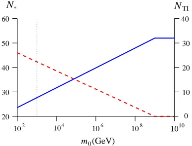
model are shown in Fig.2respectively, withg,H∗,
Γϕ and λ values from Table 1. The kink that is visible in the plot ofN∗ at aroundm0∼109GeV is
N* NTI
104
102 106 108 1010
m0(GeV)
20 30 40 50 60
10 20 30 40
[image:11.595.316.510.72.220.2]0
Fig. 2: Values of N∗ and NTI in our model, with
Γϕ≪HT I and g, Γϕ and λ values from Table 1. (Plots of Eqs. (3.16) and (4.3), withm=m0.) The
Bluesolid line depictsN∗ and theReddashed line
depictsNTI, such thatN∗+NTI= 52. The vertical
dotted line depicts values form0= 103GeV.
Parameter Value
NTI 24
[image:11.595.357.468.325.372.2]N∗ 28
Table 3: Values ofNTIand N∗ in our model, with
Γϕ ≪HTI, m0 ∼103 GeV and g, H∗, Γϕ and λ values from Table1.
a result of the fact that for m0 values larger than
this, we do not have any period of thermal infla-tion, as can be seen in the plot ofNTI. The values
ofNTIandN∗for a thermal waterfall field mass of
m0∼103GeV are shown in Table 3.
The predicted values ofnsandn′sof the model for a thermal waterfall field mass ofm0∼103 GeV
in all cases ofφ∗are the same to within at least four
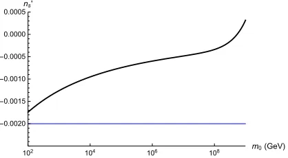
significant figures. They are also both insensitive to the value ofmψ within its allowed range.nsandn′s are shown in Table4, with them both being within current observational bounds [2]. The prediction of the model for ns and n′s and for a spectator field mass at the upper bound of mψ = 10−2 GeV are shown in Figs.3 and 4 with the parameter values of Table1.
Quantity Value
ns 0.9645
n′
s −0.001259
Table 4: Prediction for ns and n′s of the model with primordial inflation being quadratic chaotic inflation, with Γϕ≪HTI, mψ= 10−2 GeV, m0∼
102 104 106 108 m0(GeV) 0.96
0.97 0.98 0.99 1.00 1.01 1.02
[image:12.595.75.291.71.192.2]ns
Fig. 3: Prediction of the model for ns with pri-mordial inflation being quadratic chaotic inflation Γϕ≪HT I, mψ= 10−2GeV and the parameter val-ues from Table1. (A plot of Eq. (4.73), irrespective of the value of φ∗, with m=m0 and Γ =g2m0.)
The Blueand Red lines are the central value and lower/upper bounds ofns, respectively, as obtained by the Planck mission [2].
102 104 106 108 m0(
GeV)
-0.0020 -0.0015
-0.0010
-0.0005 0.0000 0.0005 ns'
Fig. 4: Prediction of the model forn′
swith primor-dial inflation being quadratic chaotic inflation, with Γϕ≪HT I, mψ= 10−2GeV and the parameter val-ues from Table1. (A plot of Eq. (4.76), irrespective of the value ofφ∗, withm=m0and Γ =g2m0.) The
Blueline is the central value of n′
s as obtained by the Planck mission [2], with the lower and upper bounds being outside the displayed range ofn′
s.
5
Conclusions
We have thoroughly investigated a new model of thermal inflation, where the thermal waterfall field is coupled to a spectator field, which is responsible for the observed primordial curvature perturbation through the “end of inflation” mechanism. We have derived a multitude of constraints for the model pa-rameters. We have found that the allowed parame-ter space for our model corresponds to a sharp pre-diction for inflationary observables, like the spectral index and its running. Taking quadratic chaotic in-flation as an example, we have obtained the values shown in Table4, which are in excellent agreement with the latest Planck data (well within 1-σ). We also found negligible tensors, withr∼10−13.
Our model works with tachyonic mass for our thermal waterfall field that is of order 1 TeV. This is rather natural for a flaton field, which corresponds to a flat direction in supersymmetry lifted by a soft mass [31–33]. The energy scale of primordial and of thermal inflation were found to be 1013GeV and
108GeV respectively, which are very reasonable
val-ues. Notice that low-scale primordial inflation en-sures that the contribution to the curvature pertur-bation of the inflaton field is negligible.
It should be stressed that the choice of model for primordial inflation may differ from our quadratic chaotic inflation example. We have found that, in the allowed parameter space, the direct contribu-tion of our spectator field tonsandn′sis negligible as ηψ ∼10−8. Thus, our expressions in Eqs. (3.2) and (3.11) becomens≃1−2ǫandn′s≃8ǫ2+ 4ǫη. Therefore, given a particular model of primordial inflation, it is straightforward to evaluate the slow-roll parametersǫandη and findnsandn′s.
The numberN∗ of remaining e-folds of
primor-dial inflation when the cosmological scales exit the horizon is drastically reduced by the presence of a subsequent period of thermal inflation. In the al-lowed parameter space,N∗≃28. This determines
the values ofǫandηand in turn the observablesns and n′
s. Note that ourN∗ is substantially smaller
than the usual 60 e-folds. Consequently, the pro-duced values of ns and n′s may vary substantially from the usual numbers corresponding to the par-ticular model of primordial inflation considered. This can render viable inflationary models that would be otherwise excluded by observations.12 This effect of
a period of thermal inflation resurrecting inflation-ary models has been employed in Ref. [34].
Note also that, in our case, thermal inflation can last much longer that the typical 10-15 e-folds, because we have considered that reheating for pri-mordial inflation occurs after thermal inflation. So, the above effect, i.e. modifying the inflationary ob-servables by changingN∗due to thermal inflation,
is intensified.
All in all, we have thoroughly investigated a new model of thermal inflation, in which the curvature perturbation is due to a spectator field coupled to the thermal waterfall field. For natural values of the model’s mass scales, we have found a sharp pre-diction of inflationary observables that depends on the chosen model of primordial inflation. Consider-ing quadratic chaotic inflation resulted in numbers that are in excellent agreement with Planck obser-vations. Our paper serves to remind readers that realistic models of inflation, in which the curvature perturbation is not generated by the inflaton field, are viable alternatives to the simple single-field
in-12
[image:12.595.79.288.320.435.2]flation paradigm.
Acknowledgements
AR thanks Anupam Mazumdar for several help-ful discussions regarding thermalization and ther-mal interaction rates. The work of KD and DHL is supported by the Lancaster-Manchester-Sheffield Consortium for Fundamental Physics under STFC grant ST/L000520/1. The early part of the work of AR was funded by an STFC PhD studentship.
References
[1] D. H. Lyth and A. R. Liddle,The Primordial Density Perturbation: Cosmology, Inflation and the Origin of Structure. Cambridge University Press, 2009.
[2] PlanckCollaboration,
P. A. R. Adeet al.,Planck 2015 results. XIII. Cosmological parameters,Astron. Astrophys.
594(2016) A13,arXiv:1502.01589v2 [astro-ph.CO];
P. A. R. Adeet al.[Planck Collaboration],
Planck 2015 results. XX. Constraints on inflation,Astron. Astrophys.594(2016) A20,
arXiv:1502.02114 [astro-ph.CO].
[3] D. H. Lyth and D. Wands,Generating the curvature perturbation without an inflaton, Phys.Lett.B524(2002) 5–14,
arXiv:hep-ph/0110002v2 [hep-ph].
[4] D. H. Lyth, C. Ungarelli and D. Wands,The Primordial density perturbation in the curvaton scenario, Phys.Rev.D67(2003) 023503,arXiv:astro-ph/0208055v3 [astro-ph].
[5] K.-Y. Choi and O. Seto,Modulated reheating by curvaton,Phys.Rev.D85 (2012) 123528,
arXiv:1204.1419v1 [astro-ph.CO].
[6] K. Dimopoulos,Can a vector field be responsible for the curvature perturbation in the Universe?,Phys.Rev. D74(2006) 083502,
arXiv:hep-ph/0607229v2 [hep-ph].
[7] K. Dimopoulos, M. Karciauskas, D. H. Lyth and Y. Rodriguez,Statistical anisotropy of the curvature perturbation from vector field perturbations,JCAP0905(2009) 013,
arXiv:0809.1055v5 [astro-ph].
[8] K. Dimopoulos,Statistical Anisotropy and the Vector Curvaton Paradigm,Int.J.Mod.Phys.
D21(2012) 1250023,arXiv:1107.2779v2 [hep-ph];
Erratum: Statistical Anisotropy and the Vector Curvaton Paradigm,Int.J.Mod.Phys.
D21(2012) 1292003,arXiv:1107.2779v2 [hep-ph].
[9] S. Yokoyama and J. Soda,Primordial statistical anisotropy generated at the end of inflation, JCAP0808(2008) 005,
arXiv:0805.4265v6 [astro-ph].
[10] H. Assadullahi, H. Firouzjahi, M. H. Namjoo and D. Wands,Modulated curvaton decay,
arXiv:1301.3439v1 [hep-th].
[11] D. Langlois and T. Takahashi,Density Perturbations from Modulated Decay of the Curvaton,arXiv:1301.3319v1
[astro-ph.CO].
[12] S. Enomoto, K. Kohri and T. Matsuda,
Modulated decay in the multi-component Universe,arXiv:1301.3787v1 [hep-ph].
[13] K. Kohri, C.-M. Lin and T. Matsuda,Delta-N Formalism for Curvaton with Modulated Decay,arXiv:1303.2750v1 [hep-ph].
[14] K. Dimopoulos, G. Lazarides, D. Lyth and R. Ruiz de Austri,Curvaton dynamics, Phys.Rev.D68(2003) 123515,
arXiv:hep-ph/0308015v1 [hep-ph].
[15] G. Dvali, A. Gruzinov and M. Zaldarriaga,
New mechanism for generating density perturbations from inflation,Phys.Rev.D69 (2004) 023505,arXiv:astro-ph/0303591v1 [astro-ph].
[16] G. Dvali, A. Gruzinov and M. Zaldarriaga,
Cosmological perturbations from
inhomogeneous reheating, freezeout, and mass domination, Phys.Rev.D69(2004) 083505,
arXiv:astro-ph/0305548v1 [astro-ph].
[17] M. Postma,Inhomogeneous reheating scenario with low scale inflation and/or MSSM flat directions,JCAP0403(2004) 006,
arXiv:astro-ph/0311563v2 [astro-ph].
[18] F. Vernizzi,Generating cosmological perturbations with mass variations,
Nucl.Phys.Proc.Suppl.148(2005) 120–127,
arXiv:astro-ph/0503175v1 [astro-ph].
[19] F. Vernizzi,Cosmological perturbations from varying masses and couplings,Phys.Rev. D69 (2004) 083526,arXiv:astro-ph/0311167v3 [astro-ph].
[20] M. Kawasaki, T. Takahashi and S. Yokoyama,
[21] D. H. Lyth,Generating the curvature perturbation at the end of inflation,JCAP
0511(2005) 006,
arXiv:astro-ph/0510443v3 [astro-ph].
[22] M. P. Salem,On the generation of density perturbations at the end of inflation, Phys.Rev.D72(2005) 123516,
arXiv:astro-ph/0511146v5 [astro-ph].
[23] L. Alabidi and D. H. Lyth,Curvature perturbation from symmetry breaking the end of inflation, JCAP0608(2006) 006,
arXiv:astro-ph/0604569v3 [astro-ph].
[24] D. H. Lyth,The hybrid inflation waterfall and the primordial curvature perturbation, JCAP1205(2012) 022,arXiv:1201.4312v4 [astro-ph.CO].
[25] D. H. Lyth and A. Riotto,Generating the Curvature Perturbation at the End of
Inflation in String Theory,Phys.Rev.Lett.97 (2006) 121301,arXiv:astro-ph/0607326v1 [astro-ph].
[26] M. Sasaki,Multi-brid inflation and non-Gaussianity, Prog.Theor.Phys.120 (2008) 159–174,arXiv:0805.0974v3 [astro-ph].
[27] F. Bernardeau, L. Kofman and J.-P. Uzan,
Modulated fluctuations from hybrid inflation, Phys.Rev.D70(2004) 083004,
arXiv:astro-ph/0403315v1 [astro-ph].
[28] T. Matsuda,Cosmological perturbations from an inhomogeneous phase transition,
Class.Quant.Grav.26(2009) 145011,
arXiv:0902.4283v3 [hep-ph].
[29] L. Alabidi, K. Malik, C. T. Byrnes and K.-Y. Choi,How the curvaton scenario, modulated reheating and an inhomogeneous end of inflation are related,JCAP1011(2010) 037,
arXiv:1002.1700v2 [astro-ph.CO].
[30] D. H. Lyth and E. D. Stewart,Cosmology with a TeV mass GUT Higgs, Phys.Rev.Lett.
75(1995) 201–204,
arXiv:hep-ph/9502417v1 [hep-ph].
[31] D. H. Lyth and E. D. Stewart,Thermal inflation and the moduli problem,Phys.Rev.
D53(1996) 1784–1798,
arXiv:hep-ph/9510204v2 [hep-ph].
[32] T. Barreiro, E. J. Copeland, D. H. Lyth and T. Prokopec,Some aspects of thermal inflation: The Finite temperature potential and topological defects,Phys.Rev.D54 (1996) 1379–1392,arXiv:hep-ph/9602263v2 [hep-ph].
[33] T. Asaka and M. Kawasaki,Cosmological moduli problem and thermal inflation models, Phys.Rev.D60(1999) 123509,
arXiv:hep-ph/9905467v1 [hep-ph].
[34] K. Dimopoulos and C. Owen,How Thermal Inflation can save Minimal Hybrid Inflation in Supergravity,JCAP10(2016) 020,
arXiv:1606.06677 [hep-ph].
[35] K. Dimopoulos and C. Owen,Modelling inflation with a power-law approach to the inflationary plateau,Phys.Rev.D94 (2016) 063518,arXiv:1607.02469 [hep-ph].
[36] A. Rumsey,Thermal Inflation with a Thermal Waterfall Scalar Field Coupled to a Light Spectator Scalar Field. Thesis,
Lancaster University, 2016.
arXiv:1610.00146v1 [astro-ph.CO].
http://inspirehep.net/record/1489131/ files/arXiv:1610.00146.pdf.
[37] K. Dimopoulos and D. H. Lyth,Models of inflation liberated by the curvaton hypothesis, Phys.Rev.D69(2004) 123509,
arXiv:hep-ph/0209180 [hep-ph].
[38] E. W. Kolb and M. S. Turner,The Early Universe, Front. Phys.69 (1990) 1.
[39] T. S. Bunch and P. C. W. Davies,Quantum Field Theory in de Sitter Space:
Renormalization by Point Splitting,Proc. Roy. Soc. Lond.A360(1978) 117–134.
[40] A. A. Starobinsky and J. Yokoyama,
Equilibrium state of a selfinteracting scalar field in the De Sitter background, Phys.Rev.
D50(1994) 6357,arXiv:astro-ph/9407016 [astro-ph].
[41] A. Ashoorioon, K. Dimopoulos, M. M. Sheikh-Jabbari and G. Shiu,
Reconciliation of High Energy Scale Models of Inflation with Planck,JCAP02(2014) 025,